
Abstract
We discuss a completely forgotten work of the geologist GF Becker on the ideal isotropic nonlinear stress–strain function (Am J Sci 1893; 46: 337–356). Due to the fact that the mathematical modelling of elastic deformations has evolved greatly since the original publication we give a modern reinterpretation of Becker’s work, combining his approach with the current framework of the theory of nonlinear elasticity.
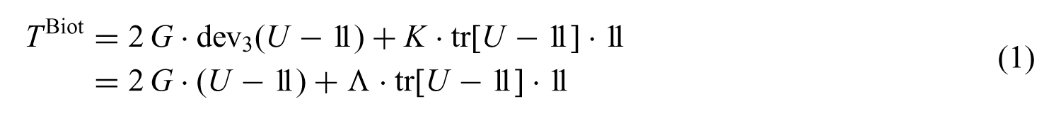
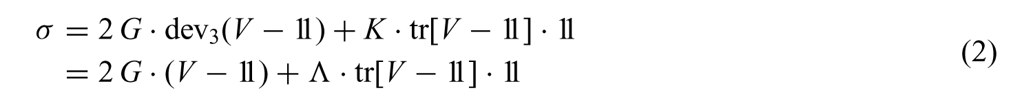
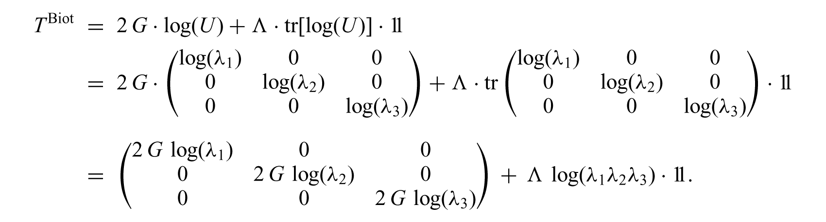
Interestingly, Becker introduces a multiaxial constitutive law incorporating the logarithmic strain tensor, more than 35 years before the quadratic Hencky strain energy was introduced by Heinrich Hencky in 1929. Becker’s deduction is purely axiomatic in nature. He considers the finite strain response to applied shear stresses and spherical stresses, formulated in terms of the principal strains and stresses, and postulates a principle of superposition for principal forces which leads, in a straightforward way, to a unique invertible constitutive relation, which in today’s notation can be written as

where TBiot is the Biot stress tensor, log(U) is the principal matrix logarithm of the right Biot stretch tensor
Here, G is the shear modulus and K is the bulk modulus. For Poisson’s number ν = 0 the formulation is hyperelastic and the corresponding strain energy

has the form of the maximum entropy function.
1. Introduction
1.1. Some reflections on constitutive assumptions in nonlinear elasticity
The question of proper constitutive assumptions in nonlinear elasticity has puzzled many generations of researchers. The problem of finding simple enough constitutive assumptions which are sufficient to characterize physically plausible behaviour of ‘completely elastic’ materials was even called ‘das ungelöste Hauptproblem der endlichen Elastizitätstheorie’ (the unsolved main problem of finite elasticity theory) by Truesdell [1]. While such assumptions can only lead to idealized material behaviour, the merits of such an ideal model were already described by H Hencky in his 1928 article On the form of the law of elasticity for ideally elastic materials [2,3]:
Like so many mathematical and geometric concepts, it is a useful ideal, because once its deducible properties are known it can be used as a comparative rule for assessing the actual elastic behaviour of physical bodies. […] While it is certainly a matter of empirical observation to determine how actual materials compare to the ideally elastic body, the law itself acts as a measuring instrument which is extended into the realm of the intellect, making it possible for the experimental researcher to make systematic observations.
The range of applicability of such an idealized response, however, must necessarily be restricted to minute strains, perhaps in the order of 1%, for otherwise we are to expect interference with non-elastic effects like plastic deformations, microstructural instabilities or bifurcations. Nonetheless, it should be formulated tensorially correct for arbitrarily large strains. It is also clear that the restriction to small elastic strains does not imply that one can use linear elasticity theory, nor that the ideal elastic response for larger stresses or strains is arbitrary. On the contrary, our idealization should work, as an ideal model, for arbitrarily large strains.
In the past, a large number of possible basic assumptions for elastic materials have been suggested in order to respond to the idealization described above. Among the most commonly accepted are:
Hyperelasticity: the existence of a strain energy function W.
Homogeneity: the strain energy W does not depend on the position in the body.
Simple material: the strain energy W = W(F) depends only on the first deformation gradient F.
Objectivity: W(Q · F) = W(F) for all Q ∈ SO(3).
Isotropy: W(F · Q) = W(F) for all Q ∈ SO(3).
Unique (up to rotations) stress-free reference state
Linearization consistent with linear elasticity theory at the reference state.
Well-posedness of the corresponding linear elasticity model in statics and dynamics.
Correct stress response for extreme strains: σ → ∞ as
Second-order behaviour in agreement with Bell’s experimental observations [4], that is, the instantaneous elastic modulus E decreases for tension and increases in the case of compression (see Figure 1).
Correct energetic behaviour for extreme strains in order to ensure invertibility of the deformation gradient F: W → ∞ for ∥F∥ → ∞ as well as W → ∞ for det(F) → 0.
Legendre–Hadamard ellipticity [12].
Baker–Ericksen inequalities [13].
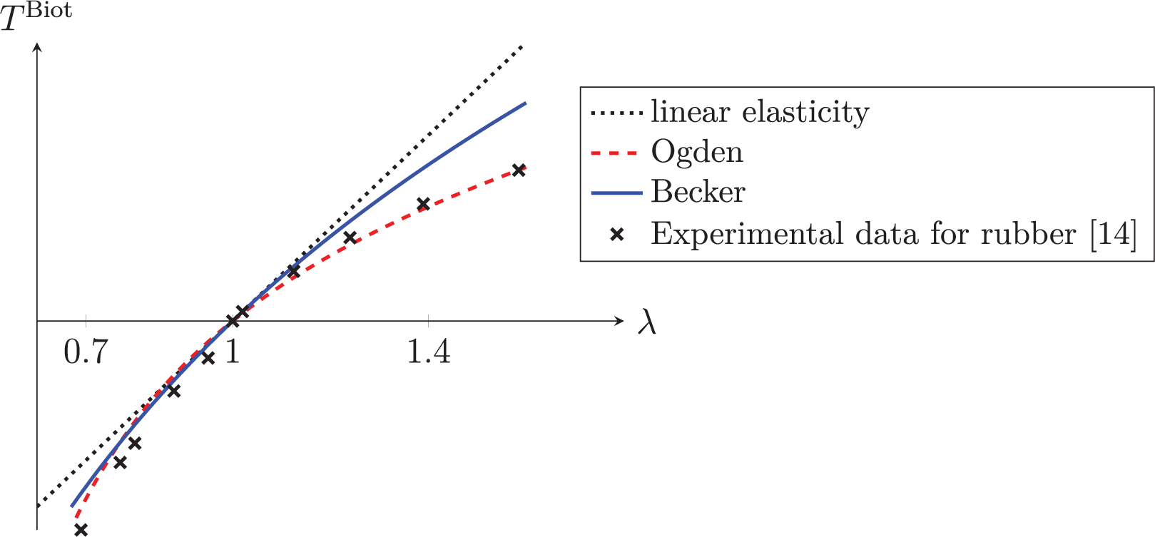
Nonlinear behaviour of incompressible elastic materials in a simple tensile stress test, drawing the Biot stress TBiot versus the principal stretch λ.
Apart from these conditions there are several properties which, while not generally viewed as necessary for an elasticity model, may be considered as constitutive assumptions for an idealized material as well:
Superposition principle: T(V1 · V2) = T(V1) + T(V2) for all coaxial stretches V1 and V2 and some corresponding stress tensor T.
Invertible stress–strain relation: the mapping E ↦ T(E) is invertible for some stress tensor T and a corresponding work-conjugate strain tensor E (if T is the Cauchy stress tensor, then this invertibility condition is satisfied for example for a variant of the compressible neo-Hookean energy [15]; if T is the Biot stress tensor, then this condition is Truesdell’s invertible force stretch (IFS) relation [16, p. 156]).
Tension–compression symmetry: T(V−1) = −T(V) for some stress tensor T (note that the classical hyperelastic tension–compression symmetry W(F) = W(F−1) is equivalent to τ(V−1) = − τ(V) for the Kirchhoff stress τ and the left stretch tensor V).
Plausible behaviour under simple homogeneous finite stresses (similar to linear elasticity):


Ordered stresses (‘greater stress corresponds to greater stretch’): (Ti − Tj) · (λi − λj) > 0 for all λi ≠ λj and some stress tensor T, where Tk are the principal stresses, that is, the principal values of T, and λk are the principal stretches (note that the Baker–Ericksen inequality can be stated as (σi − σj) · (λi − λj) > 0 for all λi ≠ λj where σ is the Cauchy stress tensor).
Simple volumetric–isochoric decoupling to ensure a suitable formulation of the incompressibility constraint.
Minimal number of physically motivated and experimentally identifiable constitutive coefficients, for example only the two isotropic Lamé constants.
Clear physical interpretation of Poisson’s number ν for finite deformations: ν = 1/2 enforces exact incompressibility (det F = 1) and ν = 0 implies no lateral contraction under uniaxial tension (as in linear elasticity).
Greatest possible extent of elastic determinacy [3, p. 19]: the stress response should not depend on a specific reference state or previously applied deformations; a similar condition was proposed by Murnaghan [17, 18], who argued that the dependence of the stress response on a specific ‘position of zero strain’ was tantamount to an ‘action at a distance’ and should therefore be avoided.
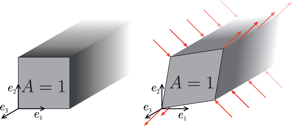
Pure shear stress should induce pure shear stretch, preserving the area A.
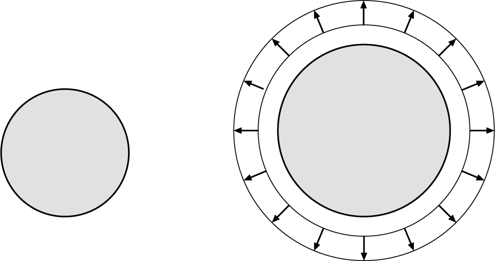
Spherical stress should induce purely volumetric stretch.
Several attempts to propose such an idealized model of elasticity can be found in the literature. Becker’s deduction can be seen as an early example of such an attempt [19].
1.2. A modern interpretation of Becker’s development
Becker, in his development of a nonlinear law of elasticity, rejects many of his contemporaries’ approaches to the problem of finite elasticity. He starts his introduction with a description of Hooke’s law, stating that apart from its original formulation (‘Strain is proportionate to the load, or the stress initially applied to an unstrained mass’ [19, p. 337]) it is often interpreted in a different way (‘Strain is proportional to the final stress required to hold a strained mass in equilibrium’ [19, p. 337]). These two different interpretations of Hooke’s law for finite deformations 1 can be expressed as
and
respectively, where
Instead, his approach to describe the deformation of an ideally elastic body can be summarized as follows: motivated by geometric considerations he postulates a connection between shear stresses and shear strains as well as between volumetric stresses and dilational strains. He then shows that every homogeneous finite deformation can be decomposed into two shear stretches and a purely dilational deformation. Finally Becker assumes that a law of superposition holds for all coaxial finite strains, allowing him to reduce the problem of a general stress–stretch relation to shears and dilations only.
Thus Becker makes a number of assumptions about the stress–stretch relation from which he then deduces a law of elasticity. His final result is a stress–stretch relation which in today’s notation can be written as

where log(U) is the principal matrix logarithm of the right Biot stretch tensor
In order to reproduce Becker’s approach in a more modern framework of elasticity theory we will therefore interpret Becker’s implicit assumptions as axioms for a law of ideal elasticity. While Sections 2 and 3 summarize Becker’s motivation for these axioms as well as some of his computations, a generalized deduction of Becker’s law of elasticity will be given in Section 4. Finally, we will investigate some basic properties of the resulting stress–stretch relation in Section 5. The notation employed throughout the article can be found in Appendix A.
While the axioms are in fact sufficient to completely characterize an isotropic stress–stretch relation uniquely up to two material parameters, it turns out that some of them may be weakened considerably without changing the result.
2. Becker’s assumptions
In order to understand Becker’s approach it is important to distinguish his (often implicitly stated) assumptions from his deduced results. Like Becker, we consider a unit cube in the reference configuration Ω0 the edges of which are aligned with an orthogonal coordinate system e1, e2, e3. Unless indicated otherwise, all matrix representations of linear mappings are given with respect to this coordinate system.
2.1. Basic assumptions
Becker’s most basic assumptions are that the stress–stretch relation is an analytic function [19, p. 342] as well as isotropic 4 [19, p. 338] and that it is possible to ‘regard strains as functions of load’ [19, p. 341], that is, that the strain-load mapping is invertible. Note that here and throughout we will interpret Becker’s ‘initial stress’ (which, for a unit cube, is equal to the load) as the Biot stress tensor [23]

where F denotes the deformation gradient, F = RU is the polar decomposition [24] of F with R ∈ SO(3) and
2.2. Pure finite shear
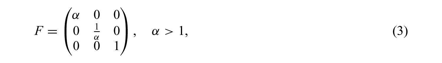
One of Becker’s main assumptions is that ‘a simple finite shearing strain must result from the action of two equal loads or initial stresses of opposite signs at right angles to one another’ [19, p. 339]. This assumption is mostly motivated by geometric considerations: if the deformation is a homogeneous pure shear of the form

Pure shear load and the corresponding shear deformation.
then the so-called planes of no distortion have a number of properties connected to the quantity α. Becker then relates these properties of strain to certain properties of stress, thereby establishing that the stress corresponding to the above shear deformation must be a pure shear stress of the form
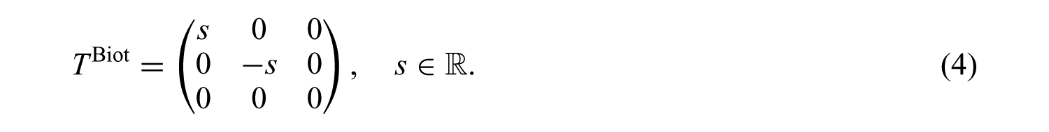
His arguments are largely based on the assumption that ‘[in] the particular case of a shear (or a pure shear) there are two sets of planes on which the stresses are purely tangential, for otherwise there could be no planes of zero distortion’ [19, p. 338].
If a Biot shear stress of the form (4) corresponds to a pure shear deformation of the form (3), then the corresponding Cauchy stress tensor σ computes to
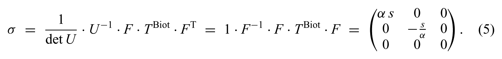
The principal Cauchy stresses are therefore σ1 = α s, σ2 = −s/α and σ3 = 0. Note carefully that Becker’s shear deformation is oriented differently: in his considerations, the contractile axis (along the eigenvector to the smaller eigenvalue 1/α) is aligned with the e1-axis. This difference is reflected in Becker’s formula −σ1α = σ2/α [19, p. 338]. For our choice of axes, the corresponding equality reads

A more detailed geometric description of this relation will be given in Section 3. More recent discussions of shear stresses and shear strains can be found in [26] and [27]. The so-called planes of no distortion also play an important role in Becker’s treatment of the rupture of rocks [28] as well as his later works on schistosity and slaty cleavage [29, 30], where properties of the planes of no distortion are linked to failure criteria for deformations beyond the range of elastic deformations. A summary of Becker’s work on yield criteria for rocks can be found in [31], while the concept of planes of no distortion and its relation to the tangential shear strain is described in a more detailed form in [32].
2.2.1. The planes of no distortion
Let F ∈ GL+(3) denote an invertible linear mapping. We call a plane
An initial plane of no distortion is only rotated by the linear mapping F, preserving the angles between two vectors as well as their lengths.
The following basic existence property can be found in [32].

with

Since Becker only considers planes of no distortion for pure shear deformations, we will assume from now on that F has the form
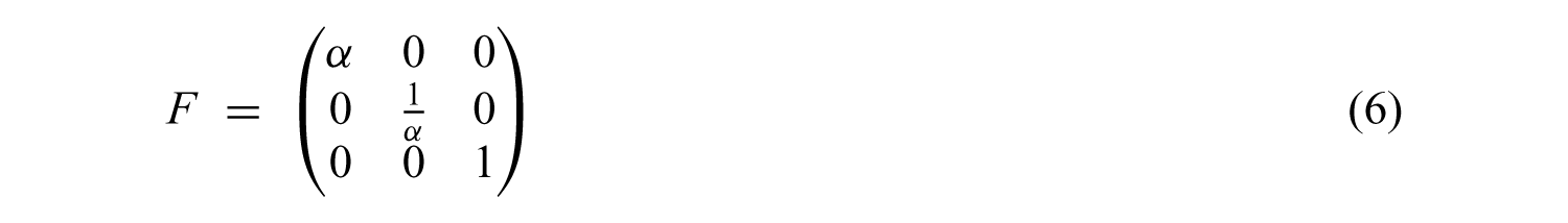
with α > 1. Then clearly λ2 = 1, hence there are two distinct planes of no distortion which can be determined by direct computation: for

to find
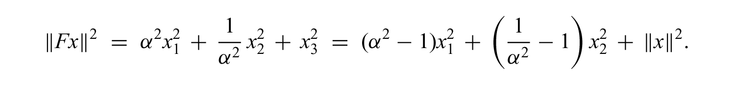
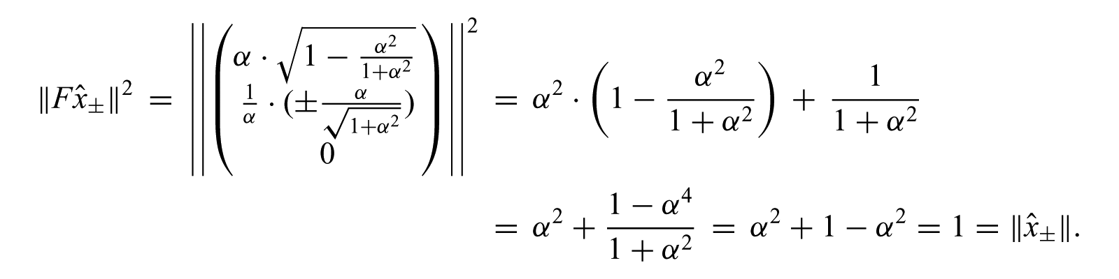
Thus the equality ∥Fx∥ = ∥x∥ is equivalent to
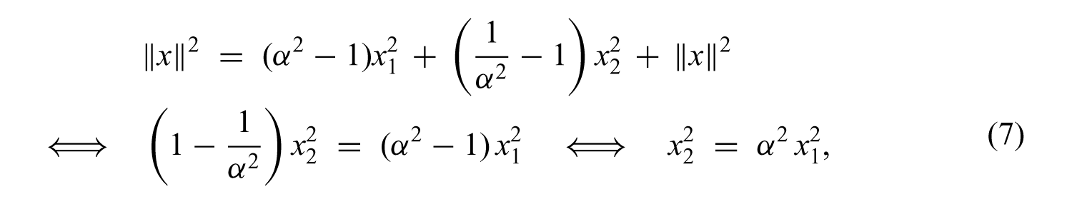
hence every
as well as two final planes of no distortion
To verify Becker’s claim that [19, p. 339] ‘[in] a finite shearing strain of ratio α, it is easy to see that the normal to the planes of no distortion makes an angle with the contractile axis of shear the cotangent of which is α’, we consider the direction of the contractile axis along the eigenvector (0, 1, 0)T = e2 corresponding to the smallest eigenvalue 1/α. Then the cotangent of the angle between this axis and a vector

are normal vectors to the planes of no distortion
This definition of the planes of no distortion is also consistent with the definition by means of the shear ellipsoid 5 given by Leith 6 in Structural geology [34]:
In a strain ellipsoid with three unequal principal axes there are only two cross-sections which are circular in outline […] These planes […] are called ‘planes of no distortion’ because they preserve a circular cross-section similar to a section of the original sphere…
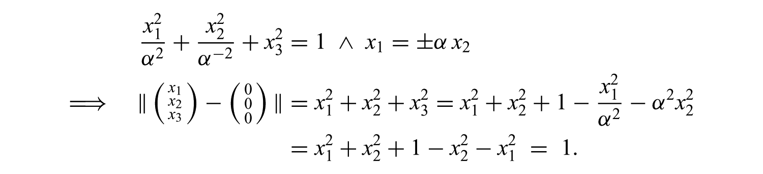
The strain ellipsoid of the deformation with principal stretches α, α−1 and 1 is defined by the equation

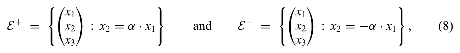
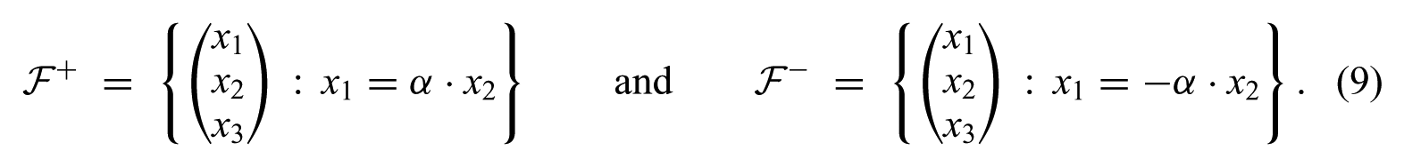
where x1 and x2 denote coordinates with respect to the tensile axis and the contractile axis respectively. The planes
2.2.2. Different characterizations of the planes of no distortion
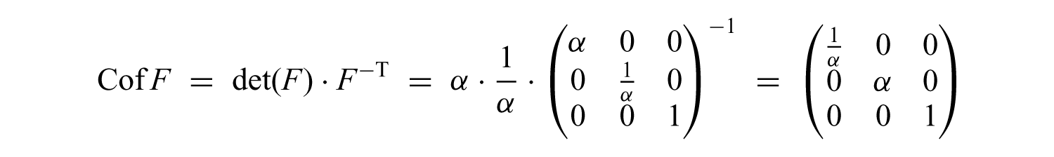
The initial planes of no distortion can also be characterized in a number of different ways, for example by means of the cofactor matrix Cof F: if the restriction of F to a plane is a rotation, then

for all x, y in the plane. Then for all x, y in the plane with 〈x, y〉 = 0 we find

Now let n denote a unit normal vector to the plane of no distortion. Then n can be represented as n = x × y with unit vectors x, y in the plane and 〈x, y〉 = 0. Since, in general,

we find

Therefore the equality ∥(Cof F)n∥ = 1 is a necessary condition for a unit normal vector n to be the normal to an initial plane of no distortion. We compute
as well as
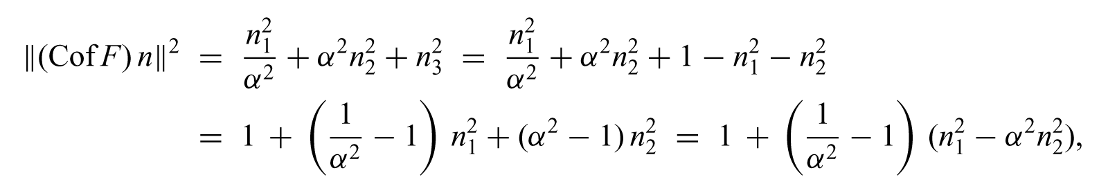
thus
for α > 1, showing that the cotangent of the angle between n and the contractile axis is ±1/α. Therefore the equality ∥(Cof F)n∥ = ∥n∥ = 1 holds only if n is a unit normal vector to a plane of no distortion. Note that this equality also implies

where B = FFT denotes the left Cauchy-Green deformation tensor.
Becker gives another important characterization of the planes of no distortion: ‘the planes of no distortion […] are also the planes of maximum tangential strain’ [19, p. 339]. In Becker’s Finite homogeneous strain, flow and rupture of rocks [28], the tangential strain of
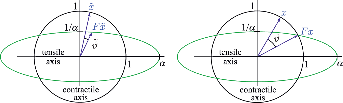
The shear ellipsoid of a deformation F, showing an arbitrary tangential strain
We will show that the planes of maximum tangential strain and the initial planes of no distortion are, in fact, identical. Let x be of the form x = (x1, x2, 0)T with

The direction x of maximum tangential strain is characterized by the angle ϑ for which tan ϑ is maximal. In order to find x it is therefore sufficient to maximize

Another visualization of the tangential strain: the shift between two parallel vertical lines under the deformation is maximal along the plane of no distortion.
since ϑ ↦ tan ϑ is monotone. Using the equality

In order to find t ∈ [−1, 1] for which the function

attains its maximum, we compute the first derivative of f to be

Thus the possible extremal points of f are 0, ±1 and

as well as f(−1) = f(0) = f(1) = 0 and f(t) ≥ 0 for all t ∈ [−1, 1], the global maxima of f are given by

Finally, in order to verify Becker’s claim that ‘the planes of no distortion […] are also the planes of maximum tangential strain’ [19, p. 339], we observe that
Thus the plane of maximum tangential strain is indeed the initial plane of no distortion.
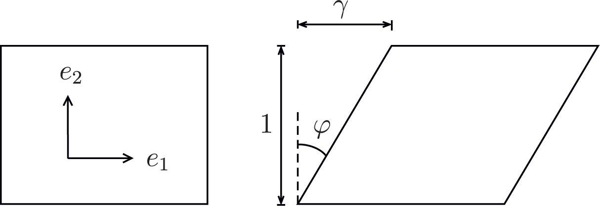
Simple glide deformation with shear angle tan φ = γ/1; horizontal lines slide relative to each other, vertical lines tilt to accommodate; originally right angles are distorted, the shear strain measures the change of angles.
2.2.3. Simple glide deformation
A homogeneous deformation F is called a simple glide if it has the form [35]

with
We examine the right Cauchy-Green deformation tensor of a simple glide, which is given by

The principal stretches λi are the singular values of F which, in turn, are the square roots of the eigenvalues of C,

and the principal axes are given by the corresponding eigenvectors of C:
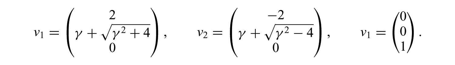
Since 1 < λ1 = 1/λ2 as well as λ3 = 1, we can interpret the simple glide as a rotated pure shear with shear ratio α = λ1, where the direction of the tensile axis is v1 and the contractile axis is given by v2. The cotangent of the angle ϑ between v2 and the e1-axis is

Hence the angle between (1, 0, 0)T = e1 and the contractile axis is

yielding another angular characterization of the shear ratio α.
2.3. Dilation
Similarly to the connection between shear stress and shear stretches, Becker further assumes that ‘dilational forces acting positively and equally in all directions’[19, p. 339] are ‘[the loads] effecting dilation’ [19, p. 342], in other words, that purely volumetric initial stresses correspond to purely dilational stretches. More precisely, this assumption can be stated in the following way: if the principal axes remain fixed, every Biot stress of the form TBiot = a · 11 with
2.4. Superposition
Becker’s most important assumption is that of a law of superposition for coaxial deformations: ‘the load sums correspond to the products of the strain ratios’ [19, p. 341]. For homogeneous, coaxial stretch tensors U1, U2 this law can be stated as

where TBiot(U) denotes the Biot stress tensor corresponding to the right Biot stretch tensor U. Here, U1 and U2 are called coaxial if their principal axes coincide.
2.4.1. The decomposition of stresses and strains
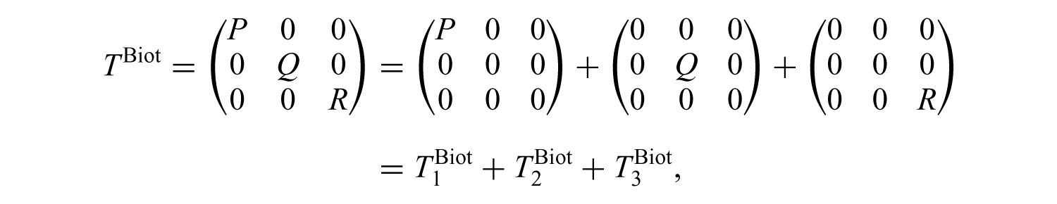
An important application of the law of superposition involves the additive decomposition of stresses and the corresponding multiplicative decomposition of stretches. Consider an initial load (i.e. a Biot stress tensor) of the form

In the case of isotropic materials, the corresponding stretches are identical for all directions orthogonal to the x1-axis for symmetry reasons, which is the case if and only if the stretch tensor corresponding to TBiot has the form

for some
In a similar way we can obtain the stretch tensors corresponding to the stresses

respectively:

for some
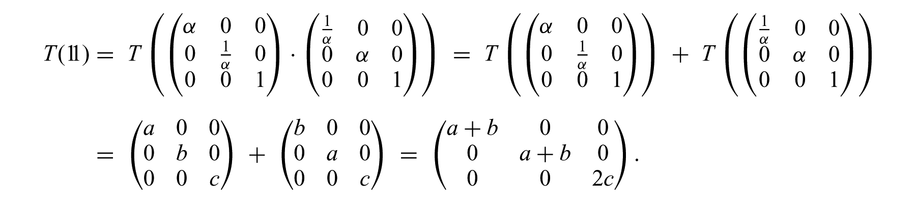
the law of superposition yields the general formula
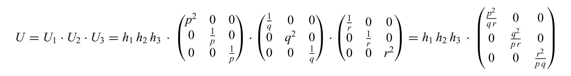
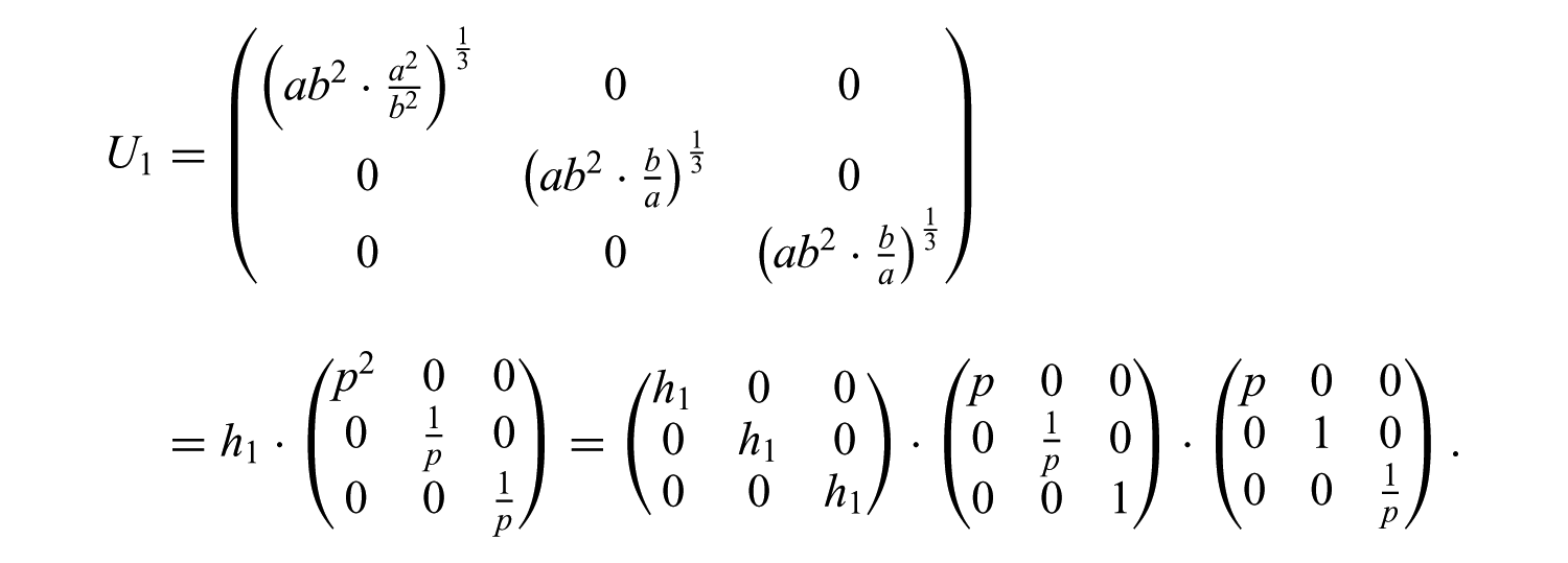
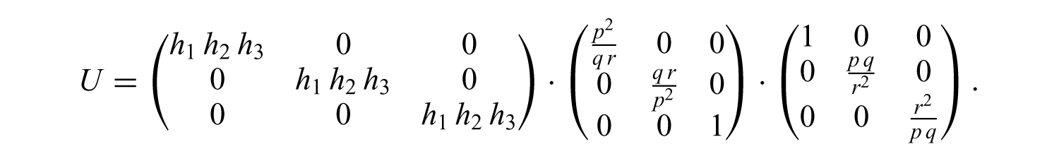
for the stretch tensor U corresponding to TBiot. Then U can be decomposed into a dilation and two shears as well:
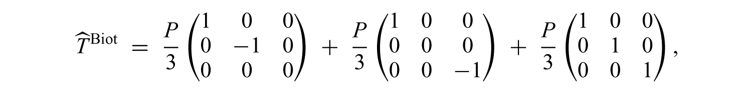
Furthermore we can find an additive decomposition
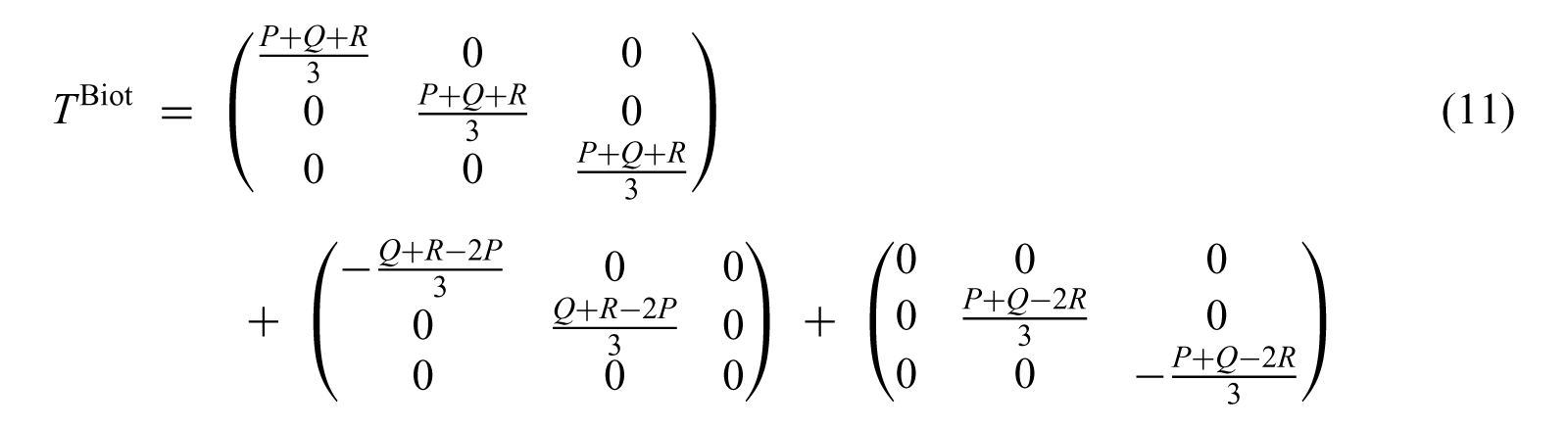
of TBiot into a spherical stress and two pure shear stresses. Note that the decomposition of U can be found in Becker’s second table [19, p. 340] while the decomposition of TBiot can be found in the third table [19, p. 340].
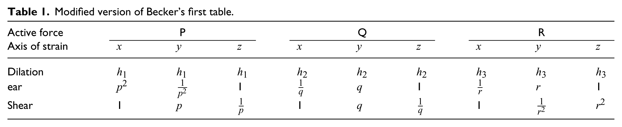
In decomposing the strains U1, U2 and U3 into a dilation and two shear strains, the planes of shear were chosen arbitrarily for every strain (or, more precisely, such that the two resulting shear ratios were identical). However, we may also choose two fixed planes (or, equivalently, fixed axes of tension and contraction) and decompose all strains into shears along the same axes:
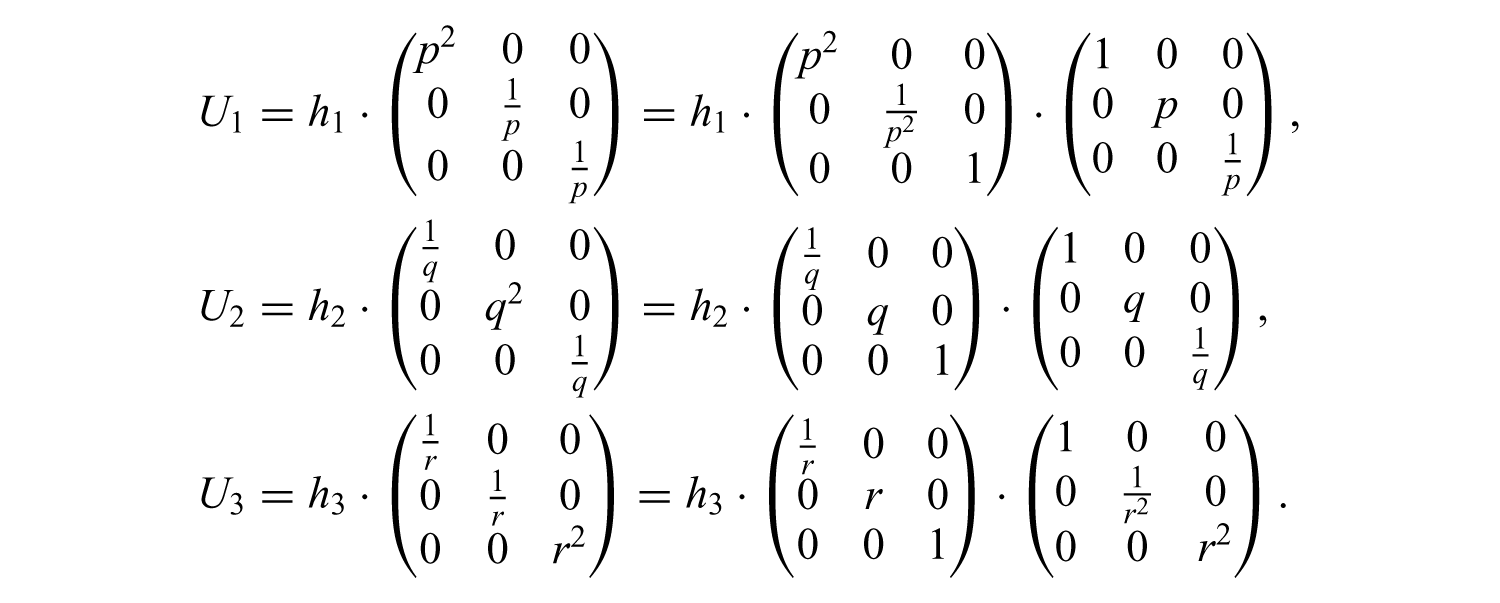
Note that the axes chosen here are identical to those chosen for the decomposition of U. Using this approach we obtain a modified version of Becker’s first table, see Table 1.
Modified version of Becker’s first table.
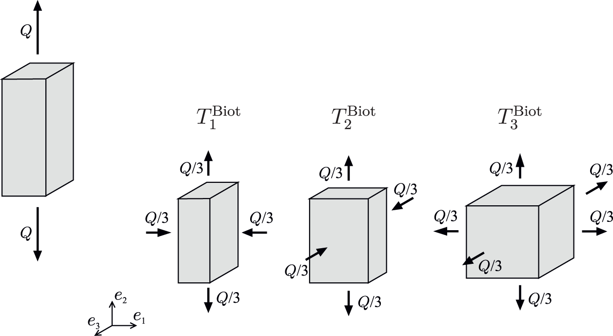
Load and deformation of the uniaxial case can be decomposed into two finite shear and a dilational mode.
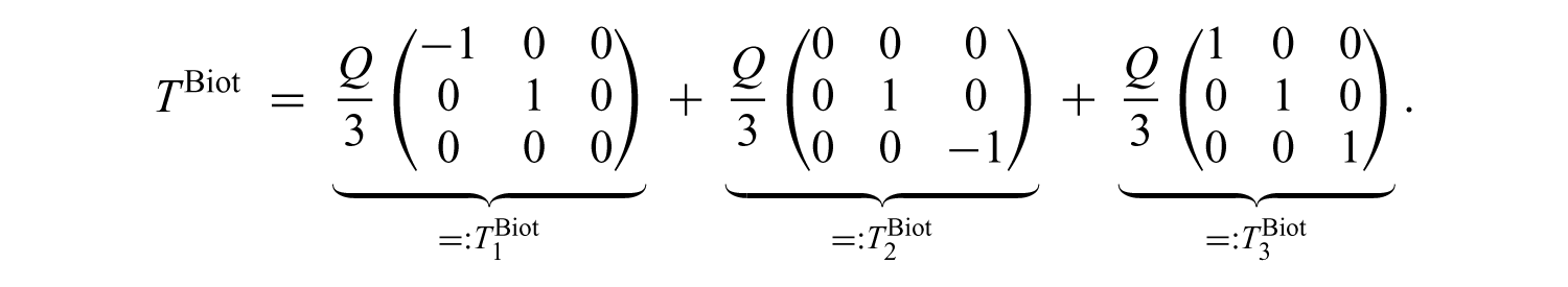
2.4.2. The uniaxial case
Consider, again, a uniaxial initial stress of the form

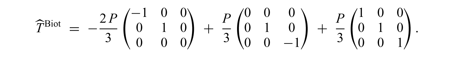
Then TBiot can be decomposed into
By Becker’s assumption the two shear stresses

respectively, while the volumetric stress

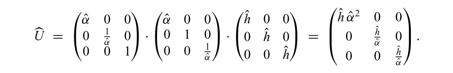
Then, according to the law of superposition, the strain corresponding to TBiot is given by

The resulting principal stretch h α2 in the direction of the applied load is referred to by Becker as the ‘length of the strained mass’ [19, p. 343] in his further computations for the uniaxial case.
Now we consider another uniaxial load given by

Then
yielding the strain
It is also possible to decompose
Note that the resulting strain is independent of this choice: since

the law of superposition yields
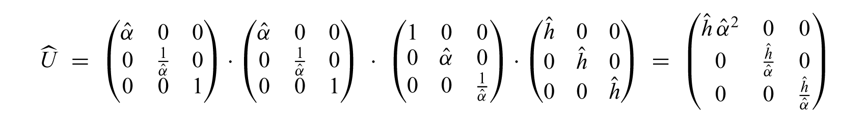
in this case as well.
2.4.3. Decomposition along fixed axes
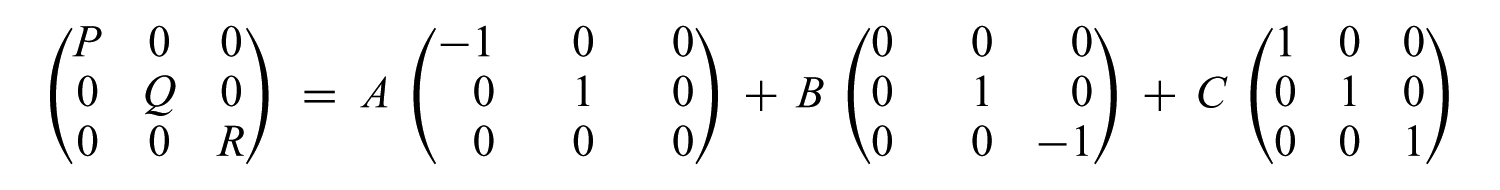
The additive decomposition of the stress tensor into a volumetric stress and two shears along fixed axes can also be expressed in basic algebraic terms. We will identify the set of all diagonal matrices in

which corresponds to two shear stresses and a volumetric stress in diagonal form, is a basis of

can be written as
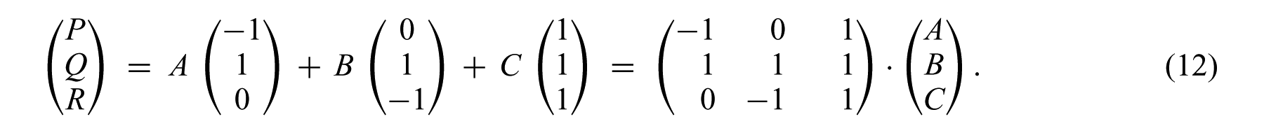
For given
by rewriting equation (12) to read
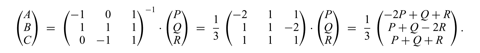
The decomposition obtained in this way is the same as given in (11).
3. Geometry and static analysis of finite shear deformation
In this section we investigate the geometric and static motivation of the relation between shear deformations and shear stresses assumed by Becker. The unit cube Ω0 aligned to the orthogonal coordinate system e1, e2, e3 in the reference configuration is considered again. We distinguish six variants of orthogonal deformation along the edges of the unit cube such that one edge preserves its length; see Figure 10.
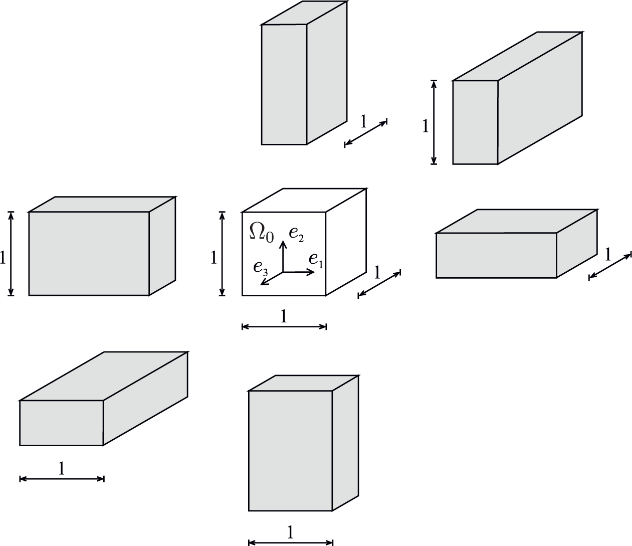
Six variants of plane, orthogonal deformation along the edges of a unit cube.
Specifying the deformation Φ α :Ω0 → Ω1 as pure finite shear with ratio α, the volume in the actual configuration Ω1 is invariant. Thus, stretching one edge in the plane of deformation by α must result in a contraction 1/α of the corresponding edge: see also Figure 11. The volume invariance holds for any intermediate configuration Ω i and goes along with the multiplicative and nonlinear behaviour of finite deformation. We consider the intermediate configuration defined by the symmetry condition

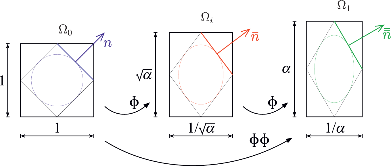
Finite shear of a unit cube.
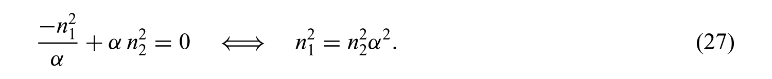
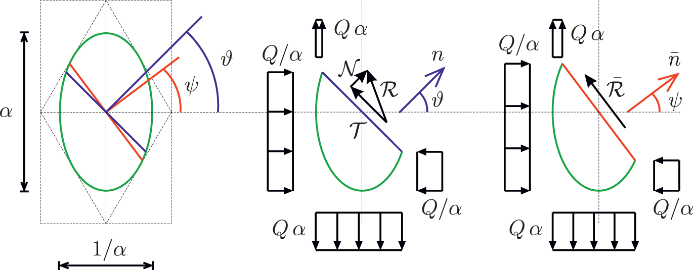
Let us inscribe a circle and a square into Ω0 as drawn on the left-hand side of Figure 11. Then
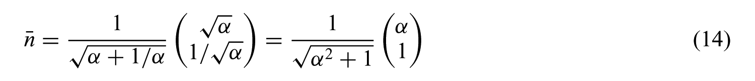
and the horizontal direction e1; see Figure 12.
Inclination ψ of the normal
Becker denotes the scalar product 〈n, ei〉 between the normal n of a plane and the coordinate axis ei as ‘direction cosines’ ni of the plane [19, p. 338]. For the normal

thus the inclination ψ of the normal

Since here the direction e1 is the contractile axis, it follows from the calculations in Section 2.2.1 that
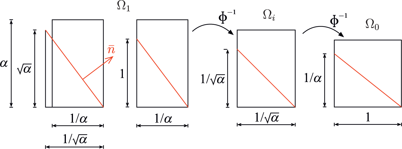
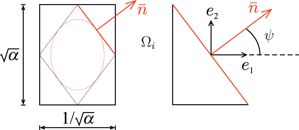
The plane of no distortion preserves its length after release of the finite shear deformation.
These properties, Becker argues, suggest that the normal component of the Cauchy stress in the directions of no distortion has to vanish, that is,

where −σ1α and σ2/α are the resultant loads; note that here, e1 is the contractile axis. From the principal Cauchy stresses in equation (17) he infers that the action of ‘two equal loads […] of opposite signs at right angles to one another’ [19, p. 339] must correspond to a simple finite shear. 8
Next, we discuss one of the six variants in Figure 10 without loss of generality. The deformation in Figure 14 results in principal stresses of horizontal and vertical direction. Defining the Cauchy stress as load per actual area, the quantity −σ1α represents a compressive force in the horizontal axis and σ2/α is a tensional force in the vertical direction. Equation (17) yields that these forces are of the same amount, say Q. Then, for a static analysis, we cut the body in Ω1 by a plane of no distortion. The lower (respectively, upper) part of the body is in an equilibrium balanced by

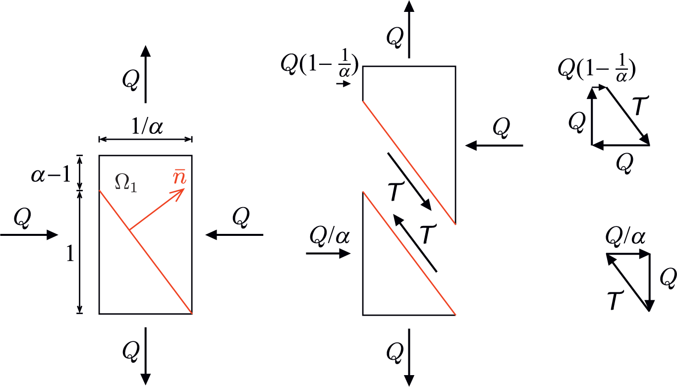
Static analysis in the actual configuration along the cut of a plane of no distortion.
The scalar product of
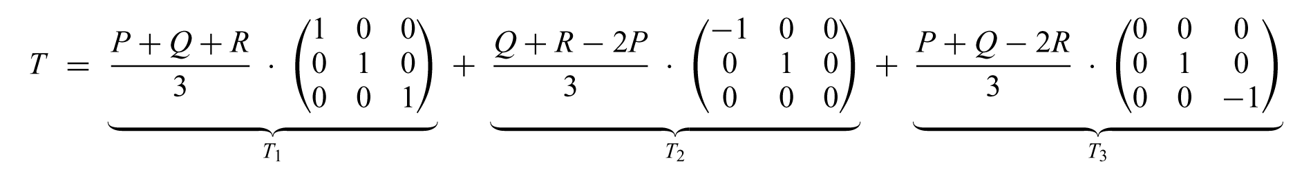
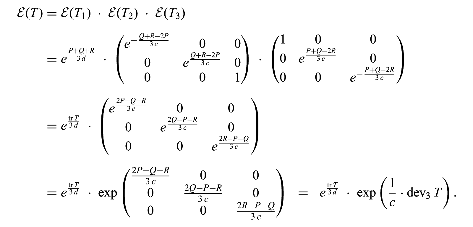
Becker concludes that the six variants of simple finite shearing in Figure 10 are caused by pairwise forces as sketched in Figure 15. This is in concordance with one of five possible invariance conditions for the definition of pure shear [36], namely that the shear tensor is a planar deviator. Note that in the case of isotropic material it is obvious to claim that P = Q = R.
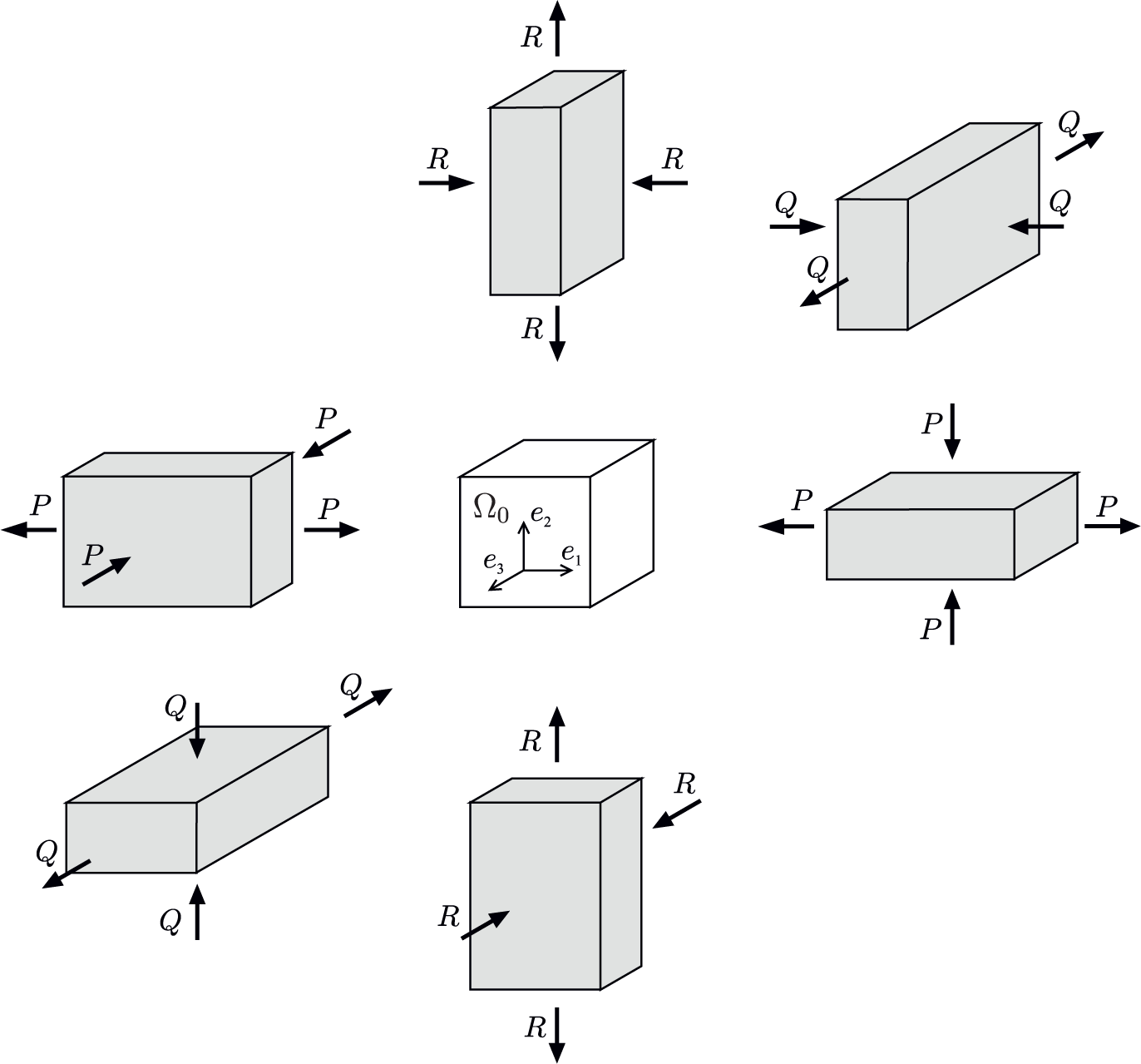
Six variants of finite pure shear and the corresponding loads.
3.1. Mohr’s stress circle for finite shear
In this section we discuss the plane of no distortion in the context of Mohr’s stress circle.
9
The Mohr circle is a graphical method to determine the stress components acting on a plane rotated against the coordinate system. Given any symmetric stress tensor in
It is important to note that the plane of maximal shear stress ρmax does not coincide with the plane of no distortion for finite shear. Considering the loading in Figure 14 together with equation (17) results in the principal stresses

Therefore, Mohr’s stress circle for the finite pure shear loading is drawn in Figure 16.
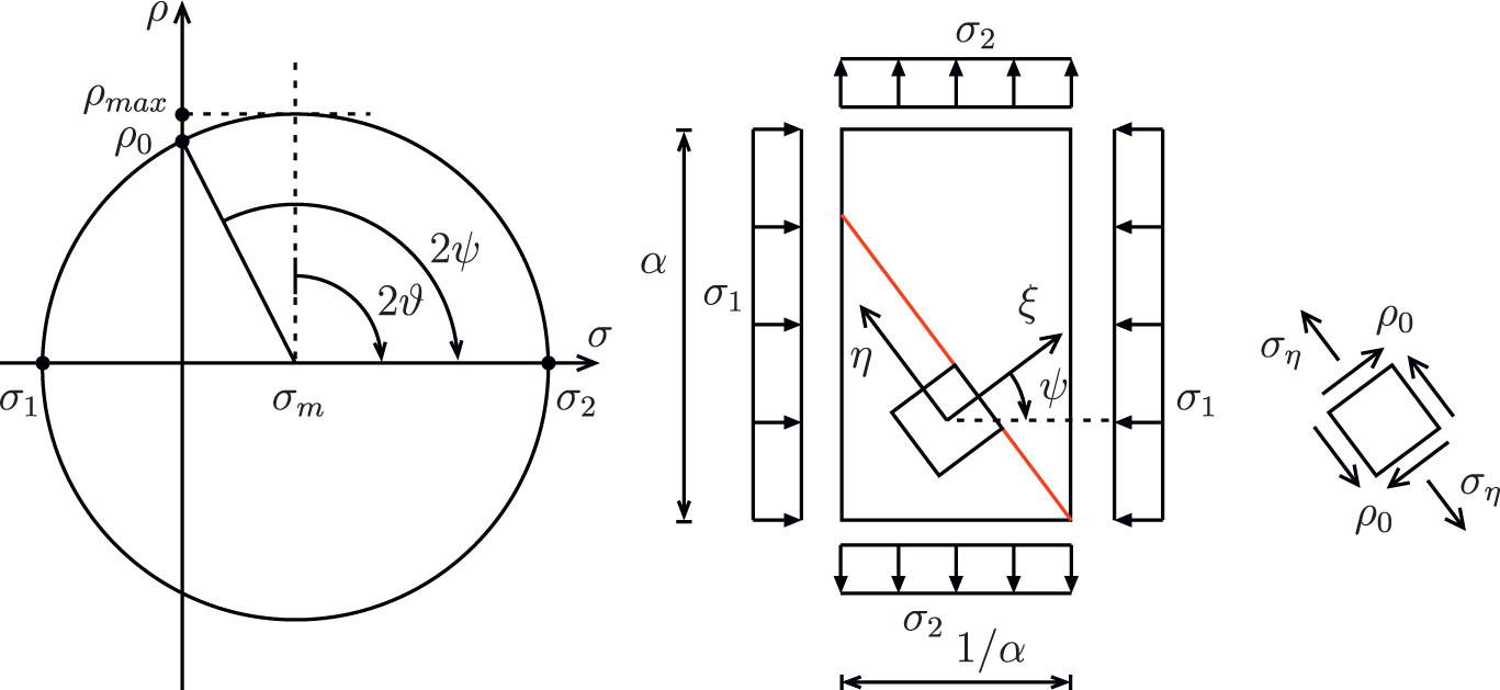
Mohr’s circle for Cauchy stresses in simple finite shear loading.
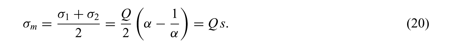
Becker introduces the quantity 2s = α − 1/α as the ‘amount of the shear’ [28]. Thus, the centre of the circle is shifted from the origin of the axis by
For α > 1 the angle ϑ = π/4 pointing to the plane of maximum shear stress ρmax does not coincide with the angle ψ describing the plane of no distortion. Demanding σξ = 0 in the plane of no distortion determines the rotation angle of the ξ, η coordinate system by
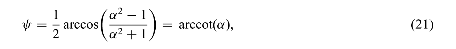
which is in accordance with equation (16). For ψ = arccot(α) the stress components are given by
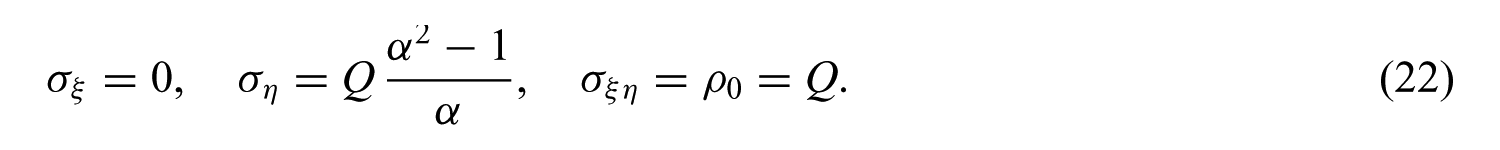
Thus, in the plane of no distortion the shear stress ρ0 is a simple function of the loading Q and independent of α.
3.2. Tangential force and failure criteria in finite shear
To discuss the tangential force in the spirit of continuum mechanics, we analyse the equilibrium of stresses in the vicinity of a point. In case of simple finite shear the surrounding of a point is a circle in Ω0 (respectively, a shear ellipse in Ω1); see Figure 11. Considering the diameter of the circle to be 1, the diameter r of the ellipse is given in terms of α and the direction cosines n1, n2 from equation (15) by

Considering the finite shear loading from Figure 14 with principal Cauchy stresses from equations (19) gives a resultant force

The normal n of the line defines the direction cosines n1 and n2 as explained in equation (15). Next, we investigate the magnitude of

The magnitude of stress

Thus the plane of maximal tangential force is due to
The planes of no distortion fulfil equation (27) and attend Becker’s discussion on failure criteria: 11 ‘Rupture by shearing is determined by maximum tangential load, not [Cauchy] stress’ [19, p. 339]; see Appendix B.4. In the present example the maximum shear stress appears in a cut inclined at ψ = 45° to the horizontal axis which does not, however, maximize the tangential load. The situation is illustrated in Figure 17.
Equilibrium and resultant
Note that the shear stress ρ0 = Q/1 = Q in the plane of no distortion is lower than the Tresca and the von Mises stresses for this kind of loading:


Thus, the inequality
It is worth mentioning that the Tresca and the von Mises stresses would account for both the loading Q and the deformation α. However, decoupling the failure criteria from the deformation suggests a basic model, which is also simple from an experimental point of view.
4. The axiomatic approach
Our aim in this section is to formulate Becker’s stress–stretch relation for ideally elastic, isotropic materials in terms of the Biot stress tensor TBiot and the right Biot stretch tensor
4.1. The basic axioms for an isotropic stress–stretch relation
Let
Of course we also assume that T fulfils the axioms stated in this section
The first two axioms are common postulates for an arbitrary stress–stretch relation
Axiom 0.1: Continuous stress response function
The function
Note that this is a weakened version of Becker’s assumption that the function relating stretch and stress is analytic.
Axiom 0.2: Unique stress-free reference configuration
The equivalence

holds.
Axiom 0.2 states that the undeformed (and possibly rotated) reference configuration is the only stress-free configuration. Again, this is a weakened version of one of Becker’s assumptions, namely that the stress response function is invertible.
Another basic assumption is that of isotropy: the response of many materials can be idealized to be independent of the direction of applied stresses.
Axiom 0.3: Isotropy
The equality

holds for all Q ∈ O(3) and
Note that isotropy is sometimes defined for Q ∈ SO(3) only. However, since −Q ∈ SO(3) for Q ∈ O(3) \SO(3), even under this narrower definition we find

for all Q ∈ O(3) \SO(3) as well.
Since the assumption of isotropy implies that
For an isotropic nonlinear elastic solid, the principal directions of Cauchy stress σ must coincide with the axes of the Eulerian strain ellipsoid. Also, to fully specify the state of strain in a material element we need only know the three principal stretches λi relative to some reference configuration and the principal directions of strain. Thus, the constitutive law is completely determined once the relations between the principal components of Cauchy stress σi and principal stretches λi are known.
Since any given

with Q ∈ O(3), where λi denote the (positive) eigenvalues of

This allows us to focus on stretches given in a diagonal representation, that is, stretches of the form

with
4.2. Becker’s three main axioms
The first two main axioms for our law of ideal isotropic elasticity refer to two special cases of deformation, pure shear and pure volumetric dilation.
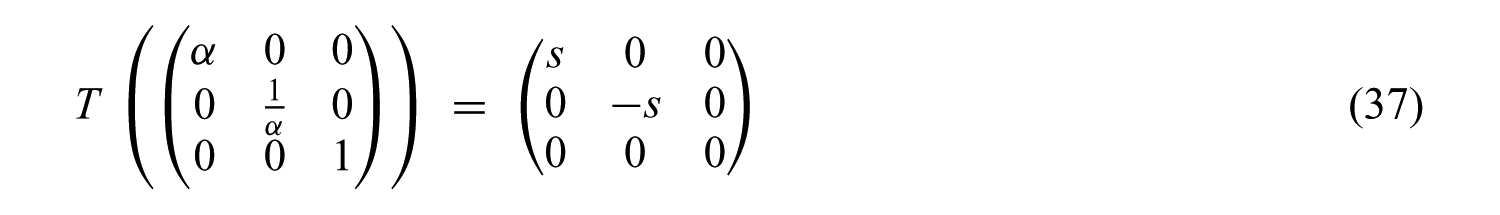
Axiom 1: Pure shear stresses correspond to pure shear stretches
For every

If T is an isotropic tensor function (Axiom 0.3), then Axiom 1 can also be stated in a more general way. Let

with

Then the two eigenvalues of

are mutually reciprocal, and thus

with

and
with

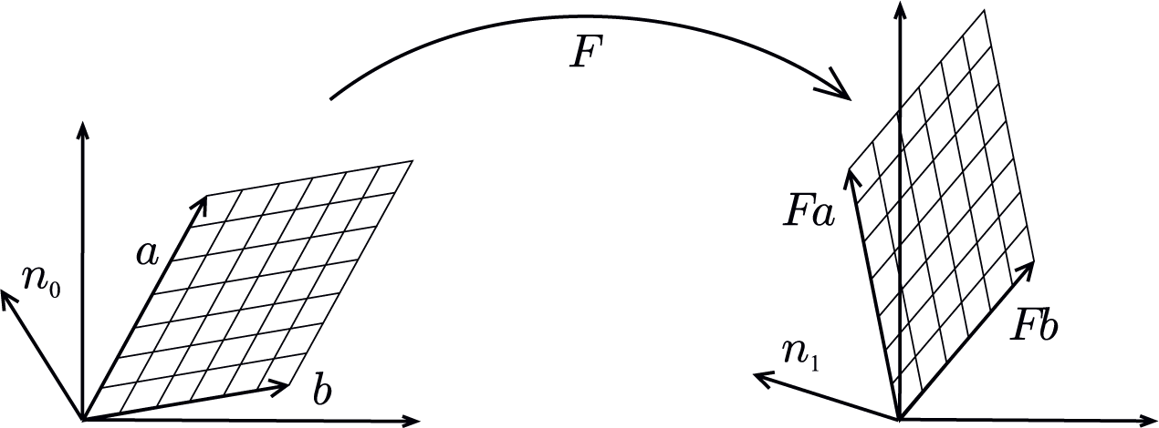
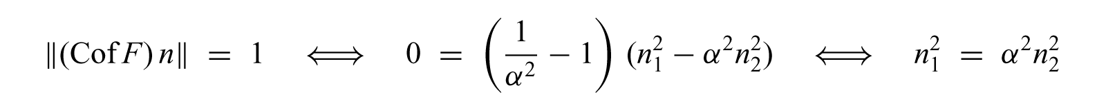
In the isotropic case, Axiom 1 may therefore be equivalently stated as follows (see Figure 2 on p. 5): for every

there exists

such that

where SL(n) denotes the group of all X ∈ GL(n) with det X = 1, and
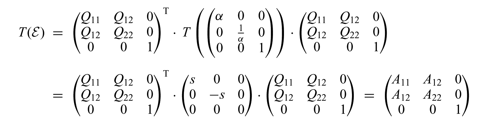
To further understand the relation between shear stress and shear stretch constituted by Axiom 1 we consider two examples. First, assume that the stress tensor T corresponding to a stretch tensor

The eigenvalues of

with Q ∈ SO(3). If
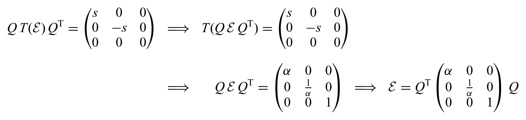
for some

with

Now assume that a deformation gradient F is a simple glide of the form

Then the right Biot stretch tensor U has the form

Since 1 is an eigenvalue of U and det U = det F = 1, the remaining eigenvalues of U must be of the form λ1 = α and λ2 = 1/α. Thus the principal stretches of the deformation are λ1 = α, λ2 = 1/α, λ3 = 1 for some

with Q ∈ O(3). Then, if the function U ↦ T(U) mapping U to a stress tensor T is isotropic and satisfies Axiom 1, we can compute
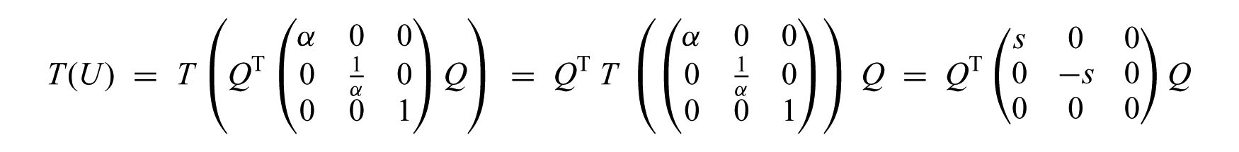
for some
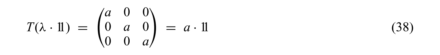
The second axiom relates spherical stresses, that is, purely normal stresses with the same magnitude in each direction, to volumetric stretches, that is, uniform stretches in all directions.
Axiom 2: Spherical stresses correspond to volumetric stretches
For every
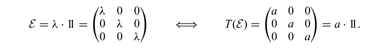
This relation between spherical stresses and volumetric stretches for isotropic elastic materials is highly intuitive: if the initial load is equal in every direction the resulting deformation should be equal in all directions as well and vice versa. However, whether this feature is true for all magnitudes of applied loads depends on the chosen constitutive framework. It is known that Axiom 2 is not satisfied for a number of well-known isotropic nonlinear elastic formulations, such as the Mooney–Rivlin energy and the Ogden type energy [26]. The loss of uniqueness of the symmetric solution is encountered in Rivlin’s cube problem [39].
While the first two axioms refer only to stresses and stretches of a specific diagonal form, our third and final axiom states a law of superposition that holds for all coaxial stress–stretch pairs. Recall that we call symmetric matrices A, B ∈ Sym(3) coaxial if their principal axes coincide, which is the case if and only if A and B are simultaneously diagonalizable as well as if and only if A and B commute.
Axiom 3: Law of superposition
Let

Note that, for an invertible stress–stretch relation, the third axiom could equivalently be stated as

for all coaxial T1,T2 ∈ Sym(3).
This law of superposition can be summarized as follows: the (multiplicative) concatenation of stretch tensors should effect the (additive) superposition of the corresponding stress tensors. This nonlinear connection is closely related to a modern approach [40] involving the theory of Lie groups: the deformation tensors correspond to the (multiplicative) group GL+(3) while the stress tensors can be represented by the (linear) Lie algebra

which is invertible with its inverse given by principal logarithm

it is to be expected that the resulting stress–stretch relation
This approach is also closely related to the later deduction of the quadratic Hencky strain energy by Heinrich Hencky, who employed a similar law of superposition to obtain a logarithmic stress response function. However, Hencky considered the superposition of stresses in the deformed configuration: the Cauchy stress σ in his 1928 article [2] as well as the Kirchhoff stress τ in his 1929 article [41] (an English translation of both papers can be found in [3]). Becker on the other hand assumes a law of superposition for initial loads: his law refers to the Biot stress tensor TBiot. A more detailed comparison of Becker’s and Hencky’s work can be found in Appendix B.1.
4.3. Deduction of the general stress–stretch relation from the axioms
We will now show that the general stress–stretch relation is determined by the given axioms up to only two constitutive parameters. Since our law of elasticity is isotropic by assumption we will mostly consider deformations given in the diagonal form

Recall from Section 4.1 that the stress–stretch relation is uniquely determined by the stress response to such deformations.
4.3.1. Basic properties
Before we explicitly compute the stress–stretch relation from the axioms, we will first deduce some basic properties. The following properties of symmetry and invertibility follow directly from the law of superposition and the uniqueness of the stress-free reference state.

where the last equality is due to Axiom 0.2.

for the energy function W and all F ∈ GL+(3). A hyperelastic stress–stretch relation is tension–compression-symmetric if and only if

for all V ∈ PSym(3), where τ denotes the Kirchhoff stress tensor.

and thus Axiom 0.2 yields
Combined with the continuity of the stress–stretch relation, the law of superposition allows us to compute the stress response to arbitrary powers of stretches. For a further discussion of non-rational powers of matrices as well as primary matrix functions in general we refer to [42].

for all

we will assume without loss of generality that
For
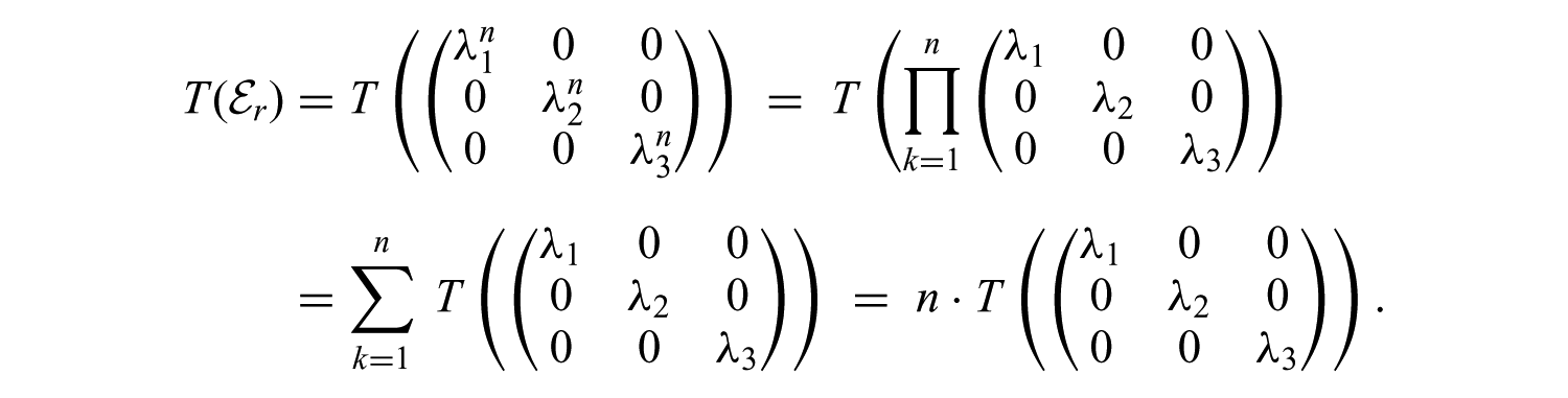
Furthermore we find

and thus

for

It is obvious that in a one-dimensional setting, Lemma 4.5 would already characterize the stress response as the logarithm to a fixed base. However, this is not immediately clear in the general case since not every stretch
Note also that the assumption of continuity is in fact necessary for the proof of Lemma 4.5.
4.3.2. Spherical stresses
While Axiom 2 relates dilations to purely spherical stresses, no assumption about the amount of stress is made. By using Lemma 4.5, however, it is easy to give an explicit formula for

for all

for some

and
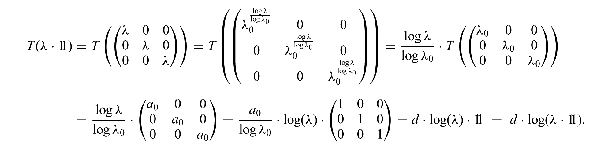
Finally, if λ = 1, then Axiom 0.2 implies T(λ·11) =λ (11) = 0 = c · log(11).

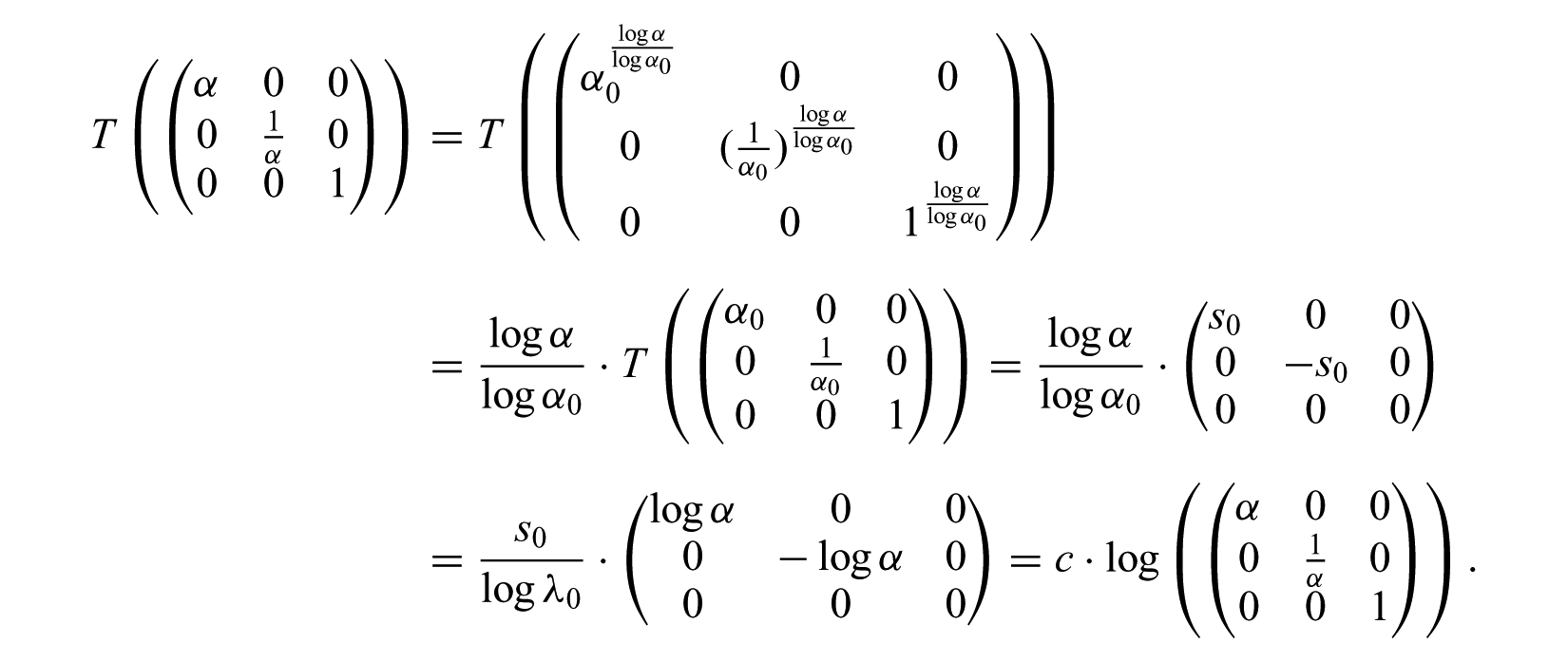
4.3.3. Shear stresses
Let us now consider a pure shear stretch of the form

with the ratio of shear
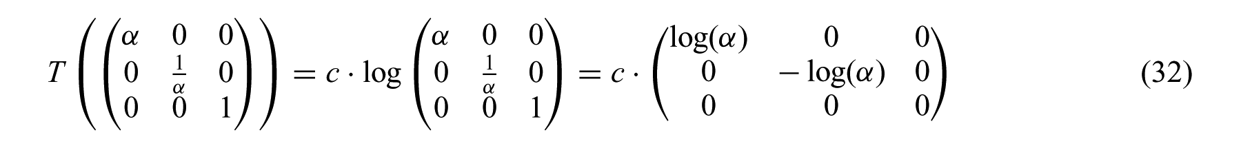
for all

according to Axiom 1, and we define c = s0/logα0.
Now let
Although Lemma 4.9 refers only to deformations without strain along the x3-axis, the following corollary shows that a similar property holds for shear deformations along the other principal axes as well.
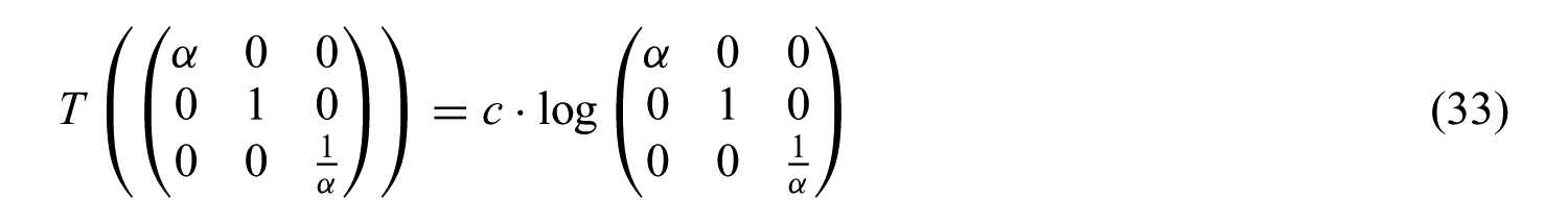
as well as
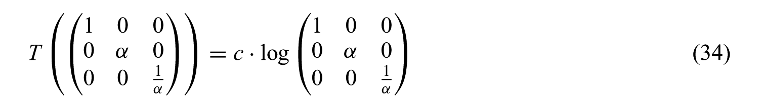
with

Then
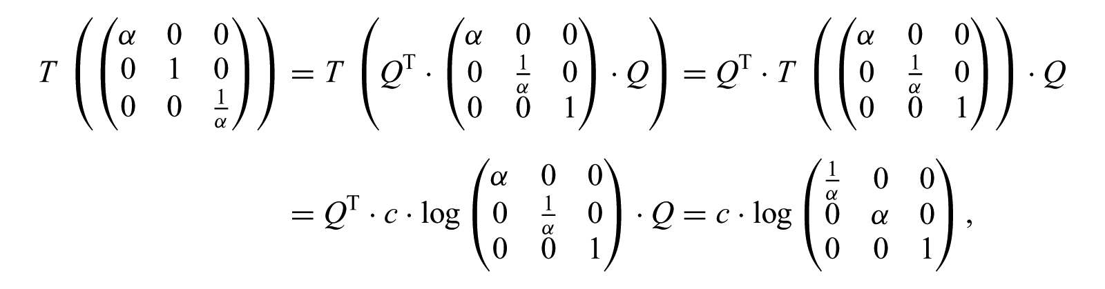
proving (33). To show (34) we let

and find
4.3.4. The general case
Finally we consider the general case of an arbitrary stretch tensor

or, equivalently, constants

for all

Then
Using the law of superposition we find
with a constant

with
hence
Thus

Finally, for arbitrary
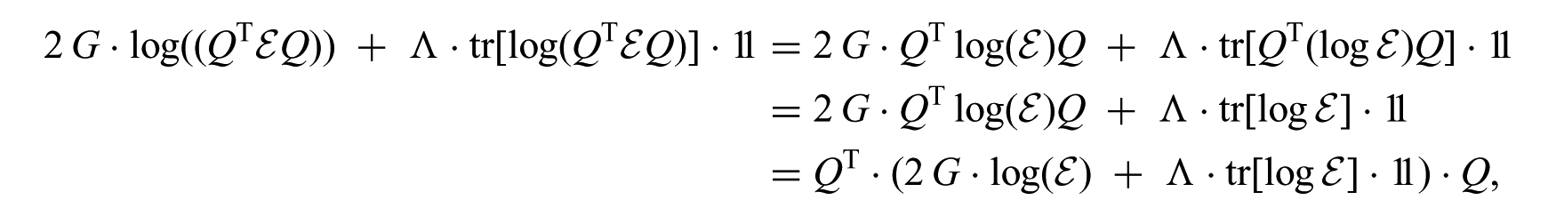
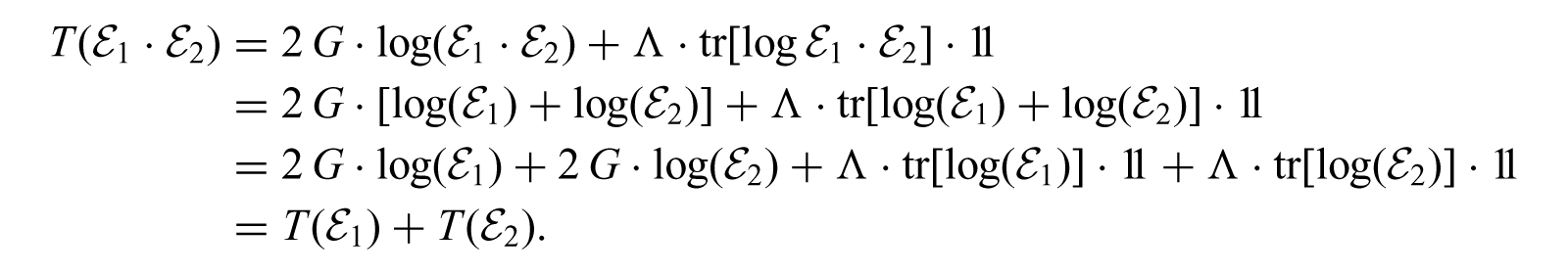
and thus we obtain equation (35) with G = c/2 and K = d/3. It is also easy to see that the restrictions G ≠ 0 and K ≠ 0 follow directly from the injectivity of the response function. Furthermore, with Λ = K − 2G/3 we obtain the equivalent representation
It remains to show that the stress response function (35) does indeed satisfy all our axioms. Since the matrix logarithm and the trace operator are continuous functions 12 on PSym(3), Axiom 0.1 obviously holds. The isotropy of the matrix logarithm immediately implies
and thus Axiom 0.3 holds as well. To show Axiom 0.2 we employ the equivalent representation formula (36): for G, K ≠ 0 we first note that the mapping

is an isomorphism from Sym(3) onto itself. Thus

if and only if
We will now consider the remaining three axioms.
Axiom 1: For
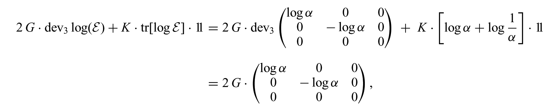
and thus Axiom 1 is fulfilled with s = 2 G log α.
Axiom 2: For
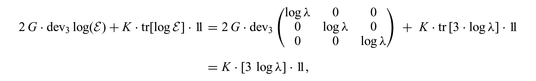
and thus Axiom 2 is fulfilled with a = 3 K log α.
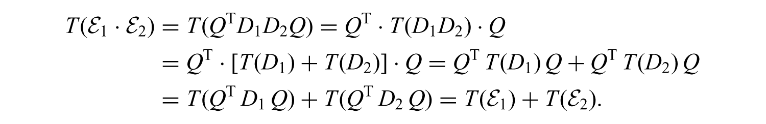
Axiom 3: First assume that

Then
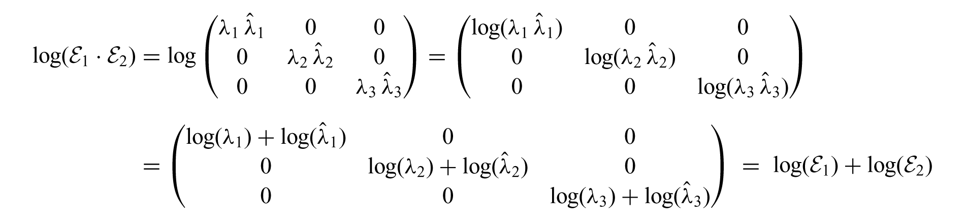
and therefore
Now let

Then
While Becker assumed Axioms 1 and 2 to hold, we will now show that they are, in fact, not necessary to characterize Becker’s law of elasticity but can be deduced from Axioms 0.1–0.3 and Axiom 3 alone.

and thus
due to Axiom 0.2. We can therefore assume without loss of generality that λ ≠ 1 ≠ α.
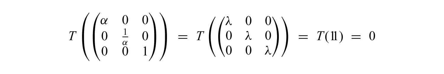
Axiom 1: Let

for some

the property of isotropy allows us to compute
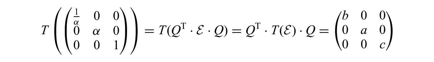
and using the law of superposition we find
Since T(11) = 0 we conclude b = −a as well as c = 0, and thus
with s = a. As was shown in the proof of Lemma 4.3, a function satisfying Axioms 3 and 0.2 is injective, hence

Axiom 2: Now let

for some

to find
Therefore a = b and b = c, and hence
with

concluding the proof.
From this lemma and Proposition 4.12, it immediately follows that the reduced set of axioms is sufficient to characterize the stress response function. This result is summarized in the following proposition.

and

for all

or, equivalently, constants

for all
If we assume beforehand that the stress response function is invertible, we can also deduce this general law in terms of the inverse stress–stretch relation: let T denote a given stress tensor of the form

Then T can be written in form of the additive decomposition
into two pure shear stresses and one spherical stress. Using Remarks 4.8 and 4.10 we compute

as well as

and

Therefore the law of superposition yields
With constants G = c/2 and K = d/3 our law of ideal elasticity can therefore be stated as

4.3.5. Becker’s stress response function
Finally, since Becker assumed Axioms 0.1 to 0.3 and 1 to 3 to hold for the Biot stress T = TBiot and the right Biot stretch tensors

or, equivalently, by

with Young’s modulus

and Poisson’s number

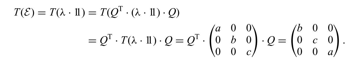
4.4. Application to other stresses and stretches
If we apply Proposition 4.15 to other coaxial stress–stretch pairs, the resulting law of elasticity will, in general, differ from that given by Becker. Two examples of such combinations are especially important: the left stretch tensor

and

for all V1, V2 ∈ PSym(3), then there exist constants

for all V ∈ PSym(3).
If the Kirchhoff stress τ is a continuous isotropic function of the left Biot stretch tensor V with

and

for all V1, V2 ∈ PSym(3), then there exist constants

for all V ∈ PSym(3).
It was shown by Hencky that only the latter of these two stress response functions constitutes a hyperelastic law of elasticity: the stress–stretch relation in equation (46) can be obtained from the quadratic Hencky strain energy

This energy function has also been given another rigorous justification, based on purely differential geometric reasoning, as the geodesic distance of the deformation gradient F to the special orthogonal group SO(3) with respect to the canonical left-invariant metric on GL+(3) [40, 43, 44]. The continuing application of the Hencky strain energy or modifications thereof is described in [12]; see also [45].
4.5. The axioms in the linear case of infinitesimal elasticity
Some of Becker’s assumptions seem to have been adapted from simple results for the linearized theory of elasticity. To explain his motivation it is insightful to discover some of these parallels. The most general stress–strain relation for isotropic homogeneous materials in the case of linear elasticity is

where σ is the linearized stress tensor and ε = sym ∇u = (1/2)(∇u + ∇uT) is the linearized strain tensor of the deformation φ(x) = x + u(x) with the displacement

similar to the first equality in equation (41).
Since the trace operator is the linear approximation of the determinant at 11, that is,

holds for sufficiently small ∥∇u∥. Therefore, the condition

can be linearized to the equation

For Λ ≠ −2G/3, this is the case if and only if

thus (linearized) isochoric deformations always correspond to trace-free stress tensors σ and vice versa, analogously to Axiom 1 for the nonlinear case. Similarly, volumetric stresses occur if and only if the strain is (linearly) volumetric (Axiom 2):
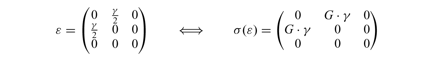
Furthermore it is easy to see that the linearized shear strain

corresponds to the shear stress (Axiom 1)

Finally, we consider two deformation gradients ∇φ1 = 11 + ∇u1 and ∇φ2 = 11 + ∇u2 with the corresponding strain tensors ε1 and ε2. Then

By omitting the higher-order term ∇u1·∇u2, we find the linear approximation

and hence the strain tensor ε corresponding to ∇φ1·∇φ2 has the linear approximation

Thus, in the linear case, the multiplicative superposition of deformation gradients corresponds to an additive composition of the strain tensors. The law of superposition (Axiom 3) can therefore be linearized to

which obviously holds for all ε1, ε2 ∈ Sym(3).
The linear analogies of the three main axioms can therefore be summarized as follows.
Axiom 1, linear version:
The equivalence
holds for all
Axiom 2, linear version:
The equivalence
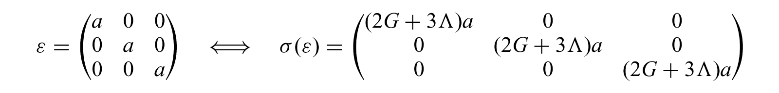
holds for all
Axiom 3, linear version:
The equality

holds for all ε1, ε2 ∈ Sym(3).
Note that many of the properties listed in Section 1.1 have linearized counterparts which are satisfied by the general linear model, for example the (linearized) tension–compression symmetry σ(−ε) = −σ(ε).
4.5.1. Linearized shear
Becker’s comments on the finite shear response show similarities to the linear case as well. We consider the linearized shear stress

with the corresponding linear shear strain 13

in the two-dimensional case. Then for given

In order to find a direction of maximum tangential linearized stress (not the tangential load), we decompose the resultant traction σ n in the direction of a given unit normal vector n into a normal and a tangential part:

where n⊥ is a unit vector normal to n. Since for such a stress the resultant ∥σ n∥2 = s2 is constant, 14 that is, independent of the unit normal n, the amount of tangential stress

assumes its maximum among all

which is minimal if and only if n1 = 0 or n2 = 0. Since the directions of the principal axes are given by the eigenvectors (1, 1)T and (1, −1)T of ε, the vectors n1 and n2 cut these axes at angles of 45°.
5. Applications and properties of Becker’s law of elasticity
5.1. Infinitesimal deformations
For small deformations the linear approximation
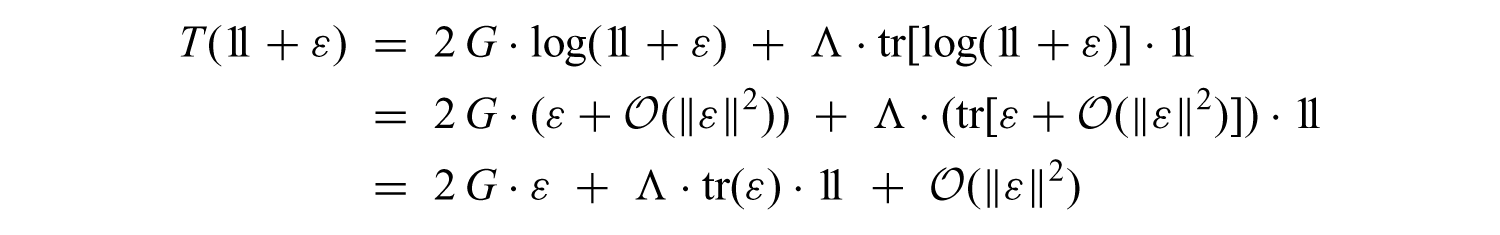
shows that the stress–stretch relation is compatible with the model of linear elasticity if and only if G and Λ are the two Lamé constants. In this case the additional constraints

follow from the uniform positivity of the linear strain energy density

5.2. Uniaxial stresses
If the initial load is given by a Biot stress tensor of the form

we can give an explicit formula for the stretch tensor U corresponding to TBiot: since tr TBiot = Q and

we can use equation (41) to find
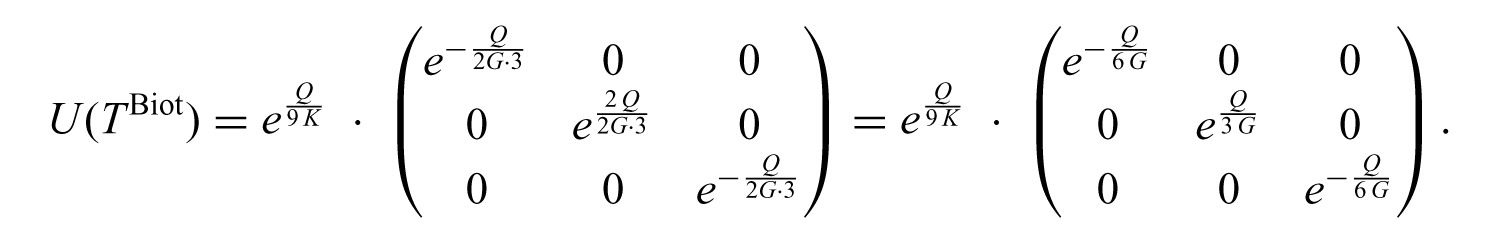
In particular, the deformation along the axis of stress is given by 14

while the deformation along the axes orthogonal to the stress axis is

The factors eQ/9K and eQ/3G appearing in equation (48) are the dilational stretch and the shear stretch, respectively, as given by Becker [19, equation (5) on page 345] as his main result. Furthermore, equation (49) shows that in the case 9K = 6G, which corresponds to ν = 0 for Poisson’s ratio ν, the stretch along the unstressed axes is 1. Therefore, as in the linear model, there is no lateral contraction in Becker’s model for ν = 0. A similar result holds for Hencky’s elastic law [46, 47].
5.2.1. Application to incompressible materials
To apply the uniaxial stress response to incompressible materials we will now consider the limit K → ∞, that is, we approximate the incompressible case through the nearly incompressible case with a sufficiently large ratio K/G. From equations (48) and (49) we readily obtain

as well as

and thus in our theory uniaxial stress induces deformations of the form

in the incompressible case. Going to the inverse we obtain the formula

where E = 3G denotes Young’s modulus for incompressible materials.
Equation (50) is identical to the uniaxial stress–stretch relation given by Imbert in 1880 as a phenomenological model for the deformation of vulcanized rubber bands under tension [48, p. 53]. Similarly, in 1893 Hartig applied the same logarithmic law to describe the uniaxial tension and compression of rubber [50]. A comparison of Becker’s results for very large strain to experimental data by Jones and Treloar for the uniaxial deformation of vulcanized rubber [14] as well as the corresponding stress responses for the quadratic Hencky energy and Ogden’s elasticity model [50] are shown in Figure 18. Another possible way to apply Becker’s law to incompressible materials is described in Section 5.5.1.
Comparison of stress responses for incompressible materials.
5.3. Becker’s law of elasticity for simple shear
Consider a simple glide deformation of the form

with γ > 0; see Section 2.2.3. Then the polar decomposition of F = R · U into the right Biot stretch tensor

Further, U can be diagonalized to
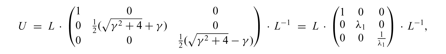
where

and
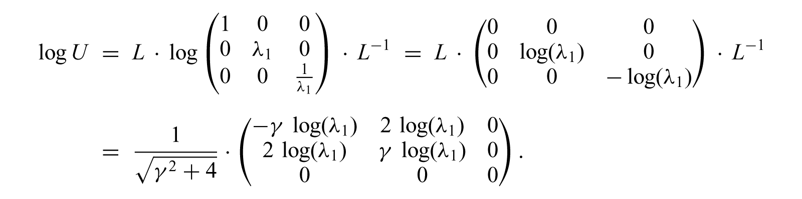
Then according to Becker’s law of elasticity, the first Piola–Kirchhoff stress tensor S1 corresponding to F computes to
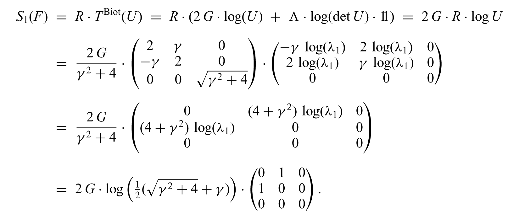
Finally, the Cauchy stress σ for the simple glide deformation F is
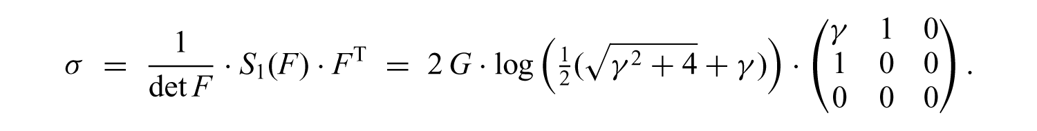
Note that σ is independent of the Lamé constant Λ. In particular, the simple shear stress σ12 corresponding to the amount of shear γ is given by

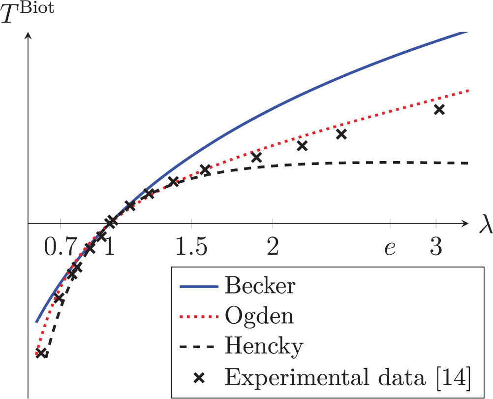
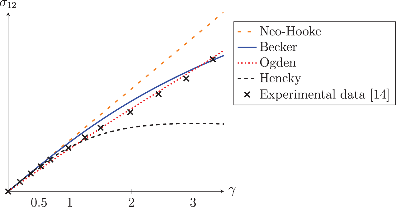
for Becker’s law of elasticity. Figure 19 shows a comparison of the simple shear stress resulting from different constitutive laws with experimental data measured by Jones and Treloar [14] for shear deformations of vulcanized rubber.
Shear stress in a simple glide deformation.
5.4. A comparison of Becker’s and Hencky’s laws of elasticity
The stress–stretch relation corresponding to the quadratic Hencky strain energy is, in terms of the Kirchhoff stress τ, the left Biot stretch tensor V and the Finger tensor B, given by

while Becker’s stress–stretch relation, expressed in terms of the Biot stress TBiot, the right stretch tensor U and the right Cauchy-Green deformation tensor C, is

Since, in general,

and

where S2 is the symmetric second Piola–Kirchhoff stress and σ is the Cauchy stress tensor, we find

where the last equality follows directly from the polar decomposition F = RU = VR of the deformation gradient F. We employ the identity C = FT F = F−1 FFT F = F−1BF to compute
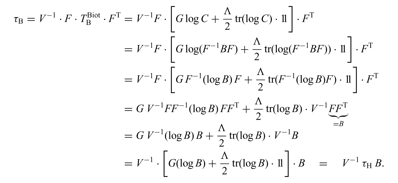
The symmetric tensors V−1, τH and B commute because their principal axes coincide, therefore

This identity allows us to obtain an upper estimate for the difference between the Kirchhoff stress corresponding to the Hencky energy and the one given by Becker’s stress–stretch relation:

where ∥·∥ denotes the Frobenius matrix norm on
5.5. Hyperelasticity
Unlike Hencky’s logarithmic stress–stretch relation, Becker’s idealized response is generally not hyperelastic for arbitrary parameters G and K. Incidentally, this result was also shown by Carroll [51], who gave an explicit example of a cycle of loading and unloading without conservation of energy, showing that the elastic behaviour modelled, in fact, by Becker’s law 16 is not path-independent.

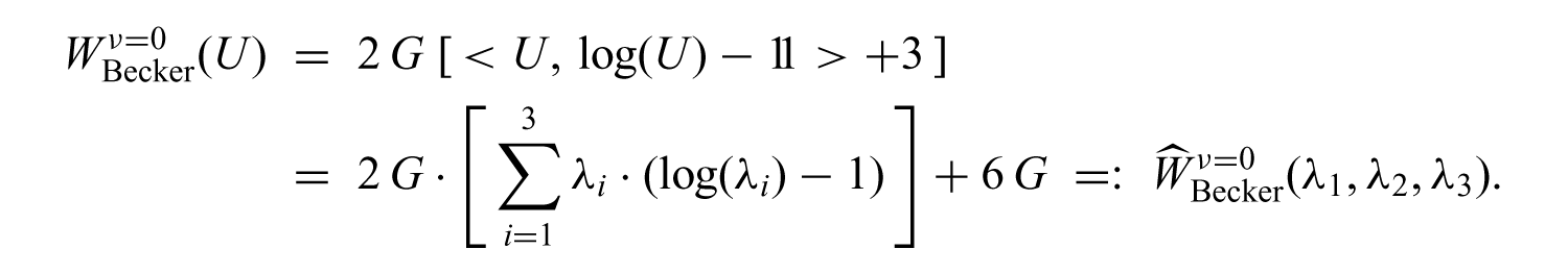
is hyperelastic if and only if Λ = 0 or, equivalently, ν = 0 for Poisson’s number ν. In this case 17 the energy is given by

which is the maximum entropy function.
However, Becker’s law is, of course, Cauchy-elastic for all admissible choices of parameters since the Cauchy stress depends only on the state of deformation.
Note that the elastic energy

holds true for Becker’s elastic law, even in the case ν = 0, c.f. Figure 20.

Energy () and Biot stress ( ) according to Becker’s law for extreme volumetric stretches λ; the tangent of
5.5.1. Comparison to the Valanis–Landel energy
In terms of the principal stretches λ1, λ2, λ3, that is, the eigenvalues of a stretch tensor U, the energy function
This energy function is identical to the Valanis–Landel energy, which was introduced in 1967 by KC Valanis and RF Landel [52]. However, the Valanis–Landel energy is used as a model for incompressible hyperelastic materials exclusively, while

where t is the (uniaxial) load, λ is the stretch and
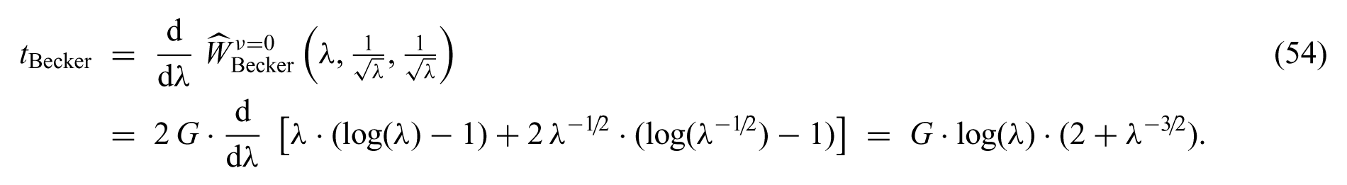
Figure 21 shows the Biot stress response for uniaxial deformations, computed from the two different applications (50) and (54) of Becker’s law to the incompressible case.
Becker’s law for the uniaxial deformation of incompressible materials, obtained via the limit case K → ∞ () and by applying the incompressibility restraint det F = 1 to the energy function ).
5.6. Becker’s law of elasticity in terms of other stresses and stretches
In Section 5.4 we already established the relation between the left Biot stretch tensor V and the Kirchhoff stress tensor τ for Becker’s law of elasticity: combining equations (52) and (51) we find

Since τ = det(V)·σ in general, the Cauchy stress tensor σ can be expressed as

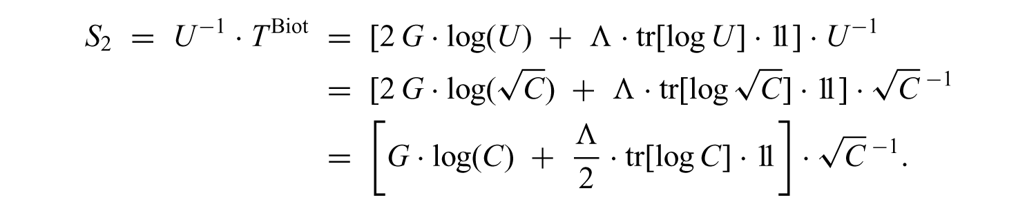
Furthermore, we can obtain a representation of the symmetric second Piola–Kirchhoff stress tensor S2 from the general formula TBiot = U · S2:

5.7. Constitutive inequalities
5.7.1. Invertibility of the force.-stretch relation
The invertibility of the force–stretch relation, also known as Truesdell’s IFS condition [16, p. 156], is fulfilled by a stress–stretch relation if and only if the mapping U ↦ TBiot(U) is invertible. Becker’s law of elasticity satisfies this condition, as was shown in Section 4.
5.7.2. The M-condition
Since the principal matrix logarithm log: PSym(3) → Sym(3) is strictly monotone [53], the Krawietz M-condition [54]

where 〈X, Y〉 = tr(YT X) denotes the canonical inner product on

that is, in the special case Λ = 0. However, it is not satisfied in the general case

for sufficiently large K > 0: choosing

we find
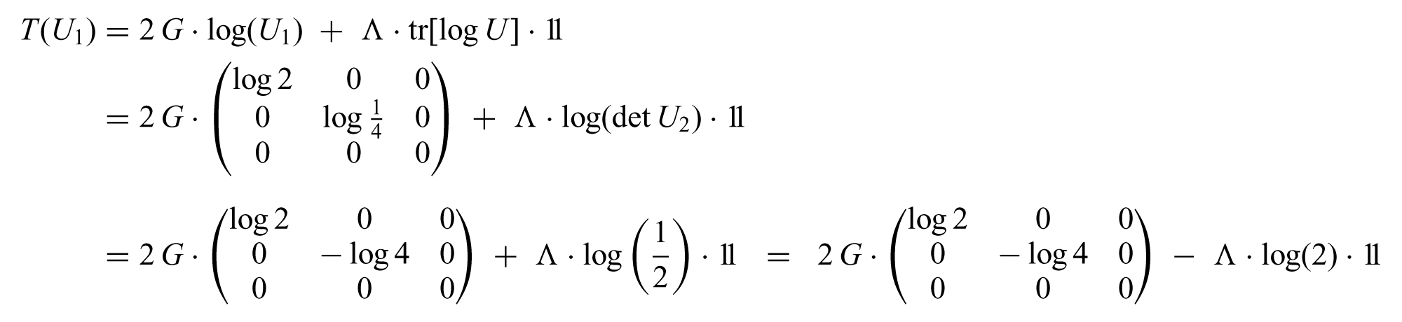
as well as T(U2) = T(11) = 0 and thus
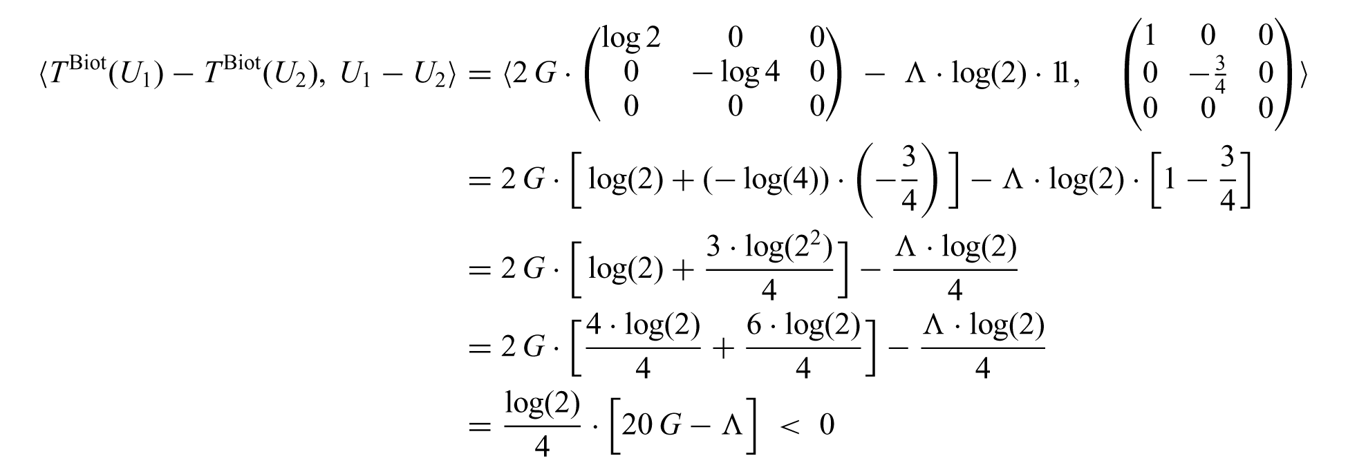
for Λ > 20 G.
5.7.3. Hill’s inequality
Since the energy function of any hyperelastic law satisfying the M-condition is convex in terms of the right Biot stretch tensor U, it follows from Section 5.7.2 that the mapping

is convex on PSym(3). However, the mapping X ↦ 〈exp(X),X − 11〉 is not convex on Sym(3). Therefore

is convex. This condition is often restated as the convexity of the mapping
5.7.4. The Baker–Ericksen inequality
A stress–stretch relation fulfils the Baker–Ericksen inequality if

where λk denotes the kth principal stretch and σk denotes the corresponding principal Cauchy stress, that is, the corresponding eigenvalue of the Cauchy stress tensor σ.

does not satisfy the Baker–Ericksen inequality for any G > 0, 3 Λ + 2 G > 0.

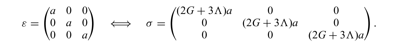
and
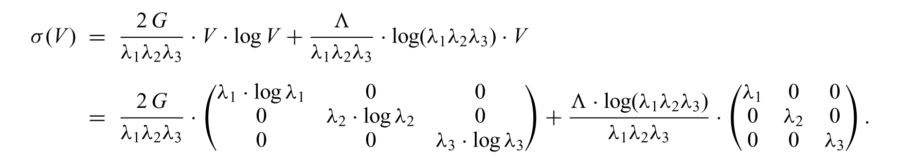
The principal stresses σk are the diagonal entries of σ, thus
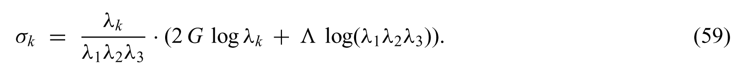
We let λ1 = 1/e, λ2 = 1/e2 and λ3 = e3 to find
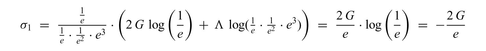
as well as
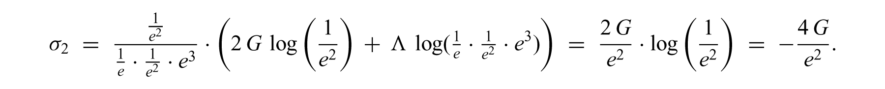
Since λ1 > λ2 we find

showing that the Baker–Ericksen inequality does not hold in this case.
Therefore Becker’s law does not satisfy the rank-one convexity condition either, since a rank-one convex stress–stretch relation always fulfils the Baker–Ericksen inequality. In contrast, Hencky’s elastic law (see (46)) does fulfil the Baker–Ericksen inequality [12].
5.7.5. The ordered force inequalities
An isotropic stress–stretch relation satisfies the ordered force inequalities (or ‘OF inequalities’) if

where λi, λj are the principal stretches of a deformation and Ti, Tj are the corresponding principal forces, that is, the eigenvalues of the Biot stretch tensor TBiot. To show that Becker’s law fulfils the OF inequalities for all G > 0, 3 Λ + 2 G > 0, we assume without loss of generality that a given stretch tensor U is in the diagonal form U = diag(λ1, λ2, λ3) and compute
The eigenvalues of Ti of TBiot corresponding to the principal stretches λi are therefore

and thus (60) can be written as
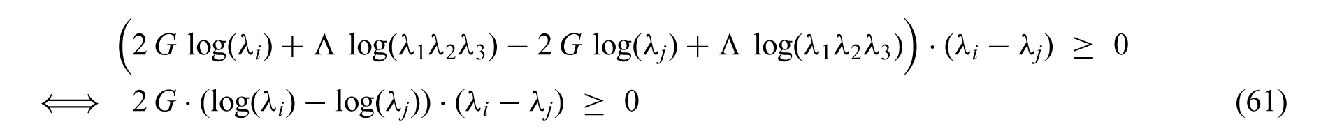
Due to the monotonicity of the natural logarithm, (61) holds for all
5.8. Existence results
The following proposition represents a basic existence result by Ciarlet [58, Theorem 6.7-1] for solutions to the so-called pure displacement problem in nonlinear elasticity.

denote the Green–Lagrange strain tensor of a deformation φ(x) = x + u(x). Moreover, assume that the constitutive law is of the form

with Λ, G > 0, where S2 denotes the second Piola–Kirchhoff stress tensor. Then for each number p > 3 there exists a neighbourhood Zp of the origin in the space Lp(Ω) and a neighbourhood Up of the origin in the subspace

of the Sobolev space W2, p (Ω) such that for each f ∈ Zp, the boundary value problem

has exactly one solution u in Up.
To show that Becker’s stress–stretch relation fulfils the conditions of Theorem 5.3 we compute
For small enough ∥C − 11∥, we can employ the series expansion

of the matrix logarithm to find
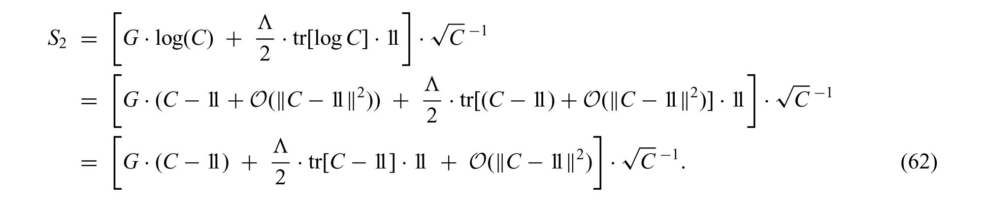
Since

for small ∥C − 11∥, (62) can be expressed as
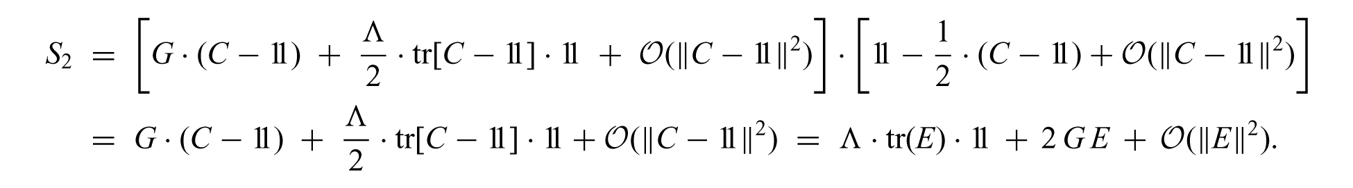
Proposition 5.3 can therefore be directly applied to Becker’s law of elasticity.
Footnotes
A. Notation
The following notation is employed throughout the article:
C = FT F = U2 right Cauchy-Green deformation tensor
B = FFT = V2 left Cauchy-Green deformation tensor
R = FU−1 = V−1F ∈ SO(3) orthogonal polar factor of the deformation gradient
σ Cauchy stress tensor, ‘true stress’
τ = det(F)·σ Kirchhoff stress tensor
S1 = det(F) σF−T first Piola–Kirchhoff stress tensor, ‘nominal stress’
S2 = det(F) F−1 σF−T symmetric second Piola–Kirchhoff stress tensor
TBiot = US2 = RTS1 Biot stress tensor
G, Λ Lamé constants
K bulk modulus
E Young’s modulus
ν Poisson’s ratio
B. Appendix
Acknowledgements
We discovered Becker’s original paper in late August 2013 and carefully transcribed it with the help of Mrs B Sacha until the end of September 2013. In January 2014 we understood the meaning of Becker’s tables on page 340 and finished a preliminary version in March 2014. We are grateful to Professor Kolumban Hutter from the ETH Zürich for his helpful remarks on the transcription.
Funding
The author(s) received no financial support for the research, authorship, and/or publication of this article.