On compressible versions of the incompressible neo-Hookean material

Abstract

We consider three different compressible versions of the conventional incompressible neo-Hookean material model. The different versions are not new and have been used in various model studies. They each give neo-Hookean behavior in an appropriate incompressible limit. The three versions each show some basic differences with respect to each other as regards the qualitative nature of the approach to the neo-Hookean limit. The purpose of this study is to exhibit these differences.

Keywords

Hyperelastic rubber elasticity nearly incompressible barely compressible penalty methods

1. Introduction

Often for the purposes of numerical computation, it is useful to develop compressible constitutive models that correspond to an existing incompressible material model. Typically, this is because an incompressible constitutive treatment may be well motivated by virtue of many materials giving an essentially incompressible response for expected mechanical loadings over standard time scales, coupled with the theoretical advantages offered by an incompressible treatment. However, once the inquiry reaches a stage where detailed computation is necessary, numerical implementation of such models generally requires a treatment where the incompressibility constraint is not enforced kinematically (as in the theoretical investigation) but is instead achieved in an approximate sense by kinetic considerations involving the relation between stress and deformation for the compressible theory [1,2]. This also has the beneficial effect of bringing the inquiry full circle by acknowledging whatever small compressibility is present in the material under study. Consequently, a variety of studies have examined the connection between truly incompressible theories and corresponding compressible theories that are nearly incompressible (see, e.g., [3 –5], additional specific reference connections are developed in what follows).

Our aim here is to contrast some of the qualitative differences in the way in which this incompressible limit is attained for the various models. For this purpose we focus on the most well-known hyperelastic material, the neo-Hookean model [6 –8]. While this is interesting in its own right, the real motivation for doing so is twofold. First, the type of methods and observations presented here are not tied to neo-Hookean behavior, and hence could be utilized for any hyperelastic incompressible material model. Even more significant, the neo-Hookean model, while itself being a model for an isotropic hyperelastic solid, often participates as a component part in a broader constitutive model that seeks to encompass a wider range of physical effects. Such effects include: polymer scission and reformation [9], fiber reinforcement [10], tissue growth [11], tissue remodeling [12], cavitation [13], material swelling [14], other porosity effects [15], material degradation [16], and chemomechanics [17]. All of the just indicated references involve modeling with a prescribed volume constraint such that there is a neo-Hookean-type term in at least part of the constitutive treatment. In a similar fashion, the combination of such effects can be considered (e.g. swelling + fibers [18], swelling + cavitation [19], swelling + degradation [20], fibers + degradation [21]). Modifying the neo-Hookean-type term in these treatments by the type of procedures described here is a logical means for interjecting a small amount of compressibility into these theories.

Incompressible hyperelasticity restricts attention to isochoric deformations; hence, J = 1 where J≡ detF and F is the deformation gradient. The stored energy density for the neo-Hookean material in the incompressible theory is

W_{nH} (I_{1}) = \frac{μ}{2} (I_{1} - 3),

(1.1)

where I₁ is the trace of C≡F^TF (the right Cauchy–Green tensor). The constraint J = 1 then restricts I₁ ≥ 3. The Cauchy stress for a neo-Hookean material is given by

T_{nH} = μ B - p_{reac} I,

(1.2)

where B≡FF^T (the left Cauchy–Green tensor) and I is the identity tensor. Here we write p_reac for the reactive constraint pressure associated with the isochoric motion constraint J = 1. This enables us to reserve the use of p for a state of hydrostatic Cauchy stress T = −pI. The constant μ corresponds to the shear modulus for small strains. This is because a simple shearing deformation

x_{1} = X_{1} + γ X_{2}, x_{2} = X_{2}, x_{3} = X_{3},

(1.3)

gives T₁₂ = μγ where T₁₂≡e₁·Te₂ is the shear stress and γ is the amount of shear. For the neo-Hookean material the relation between T₁₂ and γ is linear. Other incompressible isotropic hyperelastic models give a nonlinear relation between T₁₂ and γ. When that occurs the infinitesimal shear modulus is defined to be dT₁₂/dγ evaluated at γ = 0. This correctly correlates such a quantity with the shear modulus from the small strain theory.

In making a corresponding compressible treatment it is natural to consider compressible models with strain energy density of the form W(I₁, J) where these functions have the property that W(I₁, 1) = W_nH(I₁) (see [22]). Three such functional forms, or templates, that give W(I₁, 1) = W_nH(I₁) are the following:

W_{a} (I_{1}, J) = \frac{μ}{2} (I_{1} - 3) + a_{1} {(J - 1)}^{2} + a_{2} ln J,

(1.4)

where a₁ and a₂ are adjustable constants;

W_{b} (I_{1}, J) = \frac{μ}{2} (I_{1} J^{b_{1}} - 3) + b_{2} (J^{2} + \frac{1}{J^{2}} - 2),

(1.5)

where b₁ and b₂ are adjustable constants; and

W_{c} (I_{1}, J) = \frac{μ}{2} (I_{1} - 3) + c_{1} (J^{c_{2}} - 1),

(1.6)

where c₁ and c₂ are adjustable constants. It is to be noted that the basic template forms govern the possibilities for universal relations beyond the standard ones that are ensured by isotropic hyperelasticity [23 –25].

The next section opens with a short review of key results from the compressible theory. For each of the template forms this leads to a unique natural choice for the adjustable constants in terms of the conventional elastic constants from the small strain theory, and the resulting model forms are connected to previously considered hyperelastic models (Section 2.2). Section 2 concludes with an examination of the resulting simple shear and pressure-volume response. Section 3 looks into the qualitative form of the constant energy contours in the (I₁, J)-plane. Of specific interest here is the way in which these curves exhibit qualitatively different convergence properties in the incompressible limit. Section 4 discusses the consequences of this qualitatively different convergence for uniaxial loading. Section 5 then provides some final discussion.

2. Compressible W(I₁, J) materials

Before turning our attention to the particular template forms given above, a few general remarks are provided that are appropriate to any compressible hyperelastic model with W = W(I₁, J). The principle stretches λ₁, λ₂ and λ₃ are the square roots of the eigenvalues of C and

J = λ_{1} λ_{2} λ_{3}, I_{1} = λ_{1}^{2} + λ_{2}^{2} + λ_{3}^{2} .

(2.1)

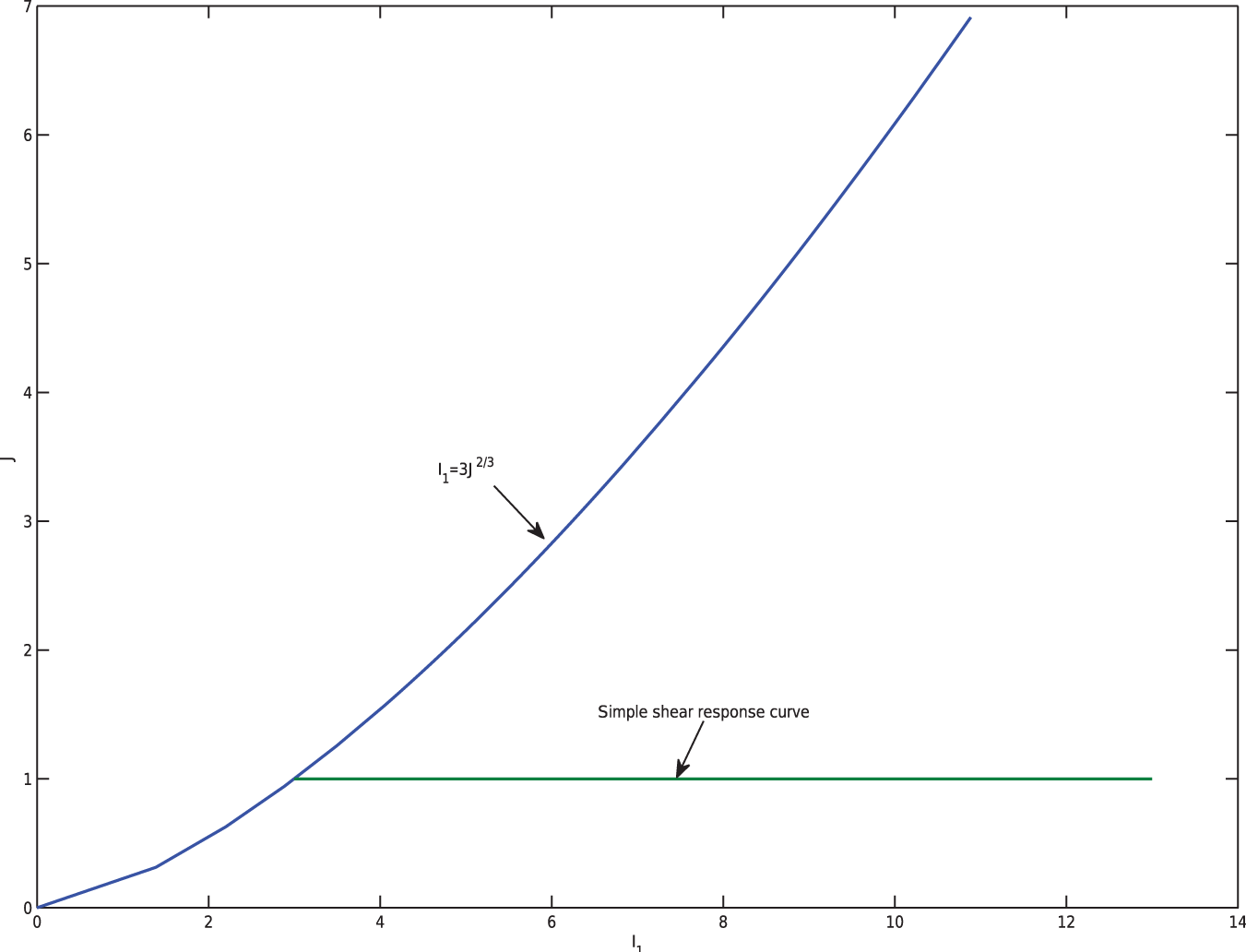
For incompressible materials J = 1 and this limits I₁ to the range I₁ ≥ 3. For compressible materials J can take on all positive values. For each J>0 the possible range for I₁ is I₁ ≥ 3J^2/3 (see [26]). This effective domain $D = {(I_{1}, J) : I_{1} \geq 3 J^{2 / 3}, J > 0}$ is shown on the right-hand side of the blue curve in Figure 1. The boundary $\partial D$ of $D$ is

I_{1} - 3 J^{2 / 3} = 0 .

(2.2)

Figure 1.

The area on the right of the blue solid curve in the first quadrant is the effective domain for (I₁, J). The left bound is the solid blue curve I₁=3J^2/3, which is also the curve for pure pressure loading. The curve for simple shear is the horizontal line J=1 starting from the left bound point where I₁=3.

The point on this curve (I₁, J) = (3, 1) corresponds to the reference configuration in which λ₁ = λ₂ = λ₃ = 1.

In general, for a W(I₁, J) compressible model the Cauchy stress tensor is

T = \frac{2}{J} F \frac{\partial W}{\partial C} F^{T} = \frac{2}{J} \frac{\partial W}{\partial I_{1}} B + \frac{\partial W}{\partial J} I .

(2.3)

A requirement that if F = I, then T = 0 (the second-order zero tensor), in other words, that the undeformed configuration is stress free, gives

{(2 \frac{\partial W}{\partial I_{1}} + \frac{\partial W}{\partial J}) |}_{(I_{1}, J) = (3, 1)} = 0 .

(2.4)

2.1. Pressure loading

Consider pure pressure loading T = −pI with symmetric deformation states F = J^1/3I. Then I₁ = 3J^2/3 and it further follows from (2.3) that p is related to J via

- p = {(2 J^{- 1 / 3} \frac{\partial W}{\partial I_{1}} + \frac{\partial W}{\partial J}) |}_{I_{1} = 3 J^{2 / 3}} \equiv - \hat{p} (J) .

(2.5)

This expression directly establishes that

\hat{p} (J) = - \frac{d}{dJ} (W (3 J^{2 / 3}, J)) .

(2.6)

The appropriate correlation to the bulk modulus from the infinitesimal strain theory is given by the derivative $- d \hat{p} (J) / dJ$ evaluated at J = 1. Let κ denote this infinitesimal theory bulk modulus, hence

κ \equiv {(- \frac{2}{3} \frac{\partial W}{\partial I_{1}} + 4 \frac{\partial^{2} W}{\partial I_{1}^{2}} + 4 \frac{\partial^{2} W}{\partial I_{1} \partial J} + \frac{\partial^{2} W}{\partial J^{2}}) |}_{(I_{1}, J) = (3, 1)} .

(2.7)

2.2. Consequences for W_a, W_b and W_c

Return now to the three template forms (1.4)–(1.6), each of which has two fitting parameters. It shall now be required that these fitting parameters are to be chosen so as to provide consistency with (2.4) and (2.7).

For W_a(I₁, J) in (1.4) these two conditions will hold if and only if

a_{1} = \frac{κ}{2} - \frac{μ}{3}, a_{2} = - μ .

(2.8)

For W_b(I₁, J) in (1.5) these two conditions will hold if and only if

b_{1} = - \frac{2}{3}, b_{2} = \frac{κ}{8} .

(2.9)

For W_c(I₁, J) in (1.6) these two conditions will hold if and only if

c_{1} = \frac{3 μ^{2}}{3 κ - 2 μ}, c_{2} = \frac{2}{3} - \frac{κ}{μ} .

(2.10)

The above parameter values will be used consistently in the following development. This gives the following three model stored energy densities:

W_{a} (I_{1}, J) = \frac{μ}{2} (I_{1} - 3) + (\frac{κ}{2} - \frac{μ}{3}) {(J - 1)}^{2} - μ ln J,

(2.11)

W_{b} (I_{1}, J) = \frac{μ}{2} (\frac{I_{1}}{J^{2 / 3}} - 3) + \frac{κ}{8} (J^{2} + \frac{1}{J^{2}} - 2),

(2.12)

W_{c} (I_{1}, J) = \frac{μ}{2} (I_{1} - 3) + \frac{3 μ^{2}}{3 κ - 2 μ} (J^{\frac{2}{3} - \frac{κ}{μ}} - 1) .

(2.13)

By construction, each of the hyperelastic material models (2.11)–(2.13) will behave for small strains like an isotropic linear elastic model with bulk modulus κ. The equivalent of model W_a is proposed in [27] and [28]; this form is subsequently considered in [29 –31]. Model W_b, with its term of the form I₁/J^2/3, is motivated by considerations discussed by Flory in [32] so as to separate the pure volumetric effect from the other aspects of the deformation. Such considerations are subsequently invoked in [22, 33 –36]. The works [37, 38] explore some commonly used volumetric parts, some of which are similar to that in W_b. The basis for model W_c follows from [39]; this model is subsequently mentioned in [30] and used in [40, 41].

Here it is useful to remark that the original templates (1.4) and (1.6) for W_a and W_c are of the form W(I₁, J) = W_nH(I₁) + ψ(J) = μ/2(I₁−3) + ψ(J) with two different template expressions for ψ(J). Such models are special forms of the general Blatz–Ko material model [42, 43]. After choosing the fitting parameters to be consistent with (2.4) and (2.7) such models require that the derivative of the function ψ(J) obey ψ′(1) = −μ. Hence, these ψ(J) are not minimized at J = 1. Thus, in neither case does the function ψ(J) by itself provide a straightforward penalization of volume departure from J = 1. In contrast the model (2.12) for W_b is of the alternative form W(I₁, J) = W_nH(I₁/J^2/3) + ψ(J), which is not a Blatz–Ko form, and this ψ(J) is minimized at J = 1.

2.3. Simple shear response

The simple shearing deformation (1.3) generates right Cauchy–Green deformation tensor

B = (1 + γ^{2}) e_{1} \otimes e_{1} + γ (e_{1} \otimes e_{2} + e_{2} \otimes e_{1}) + e_{2} \otimes e_{2} + e_{3} \otimes e_{3},

(2.14)

in turn giving J = 1 and I₁ = 3 +γ². In the (I₁, J)-plane of Figure 1 the curve for simple shear response is the horizontal line J = 1 with I₁ ≥ 3. For this deformation it follows from (2.3) that the Cauchy stress for the three models (2.11)–(2.13) is given by

T_{a} = T_{c} = μ (B - I) and T_{b} = μ (B - (1 + \frac{1}{3} γ^{2}) I), (simple shear) .

(2.15)

Recall that the Poynting relation does not allow the simultaneous vanishing of all normal stress components in simple shear with nonzero γ. Here the model W_b gives T₁₁ = 2μγ²/3>0 and T₂₂ = T₃₃ = −μγ²/3 < 0. Conversely the models W_a and W_c both give T₁₁ = μγ²>0 and T₂₂ = T₃₃ = 0. The two different forms for the simple shear deformation stress tensor in (2.15) match exactly with the general neo-Hookean result (1.2) upon suitable choice of the neo-Hookean reactive pressure p_reac. Turning to the shear stress T₁₂, in all three compressible models T₁₂ = μγ which is the same relation as that for a neo-Hookean material. This also gives that

μ = {\frac{{dT}_{12}}{d γ} |}_{γ = 0} = 2 {\frac{\partial W}{\partial I_{1}} |}_{(I_{1}, J) = (3, 1)},

(2.16)

which in turn confirms that μ in all three models (2.11)–(2.13) corresponds to the infinitesimal strain shear modulus.

This formally establishes that the κ and μ in all three models (2.11)–(2.13) correspond to the bulk and shear modulus from the infinitesimal theory. It therefore follows that all other isotropic elastic constants can be determined a priori from these moduli. For example, a finite deformation uniaxial load analysis suitably linearized to the small strain regime will of necessity predict Young’s modulus E = 9κμ/(3κ + μ) and Poisson’s ratio ν = (3κ − 2μ)/(6κ + 2μ). We remark that our usage of the symbols μ, κ, E and ν is restricted to denoting the various linear elasticity constants from the isotropic theory. While the hyperelastic theory naturally lends itself to generalizing these constants to functions of stretch [31, 43], we do not pursue such a generalization here.

In what follows it will occasionally be useful to normalize by shear modulus μ and we shall use overbar to indicate this. For example:

\bar{W} = W / μ, \bar{T} = T / μ, \bar{κ} = κ / μ, \bar{E} = E / μ .

(2.17)

Then

ν = \frac{3 \bar{κ} - 2}{6 \bar{κ} + 2}, \bar{κ} = \frac{2 (1 + ν)}{3 (1 - 2 ν)},

(2.18)

and the incompressible limit corresponds to $\bar{κ} \to \infty$ or, equivalently, ν→ 1/2. Although the admissible thermodynamic range for the Poisson ratio is −1 ≤ ν ≤ 1/2 recall that the standard range for consideration is 0 ≤ ν ≤ 1/2 and, hence, $\bar{κ} \geq 2 / 3$ . This standard range will be considered in what follows.

2.4. Pressure-volume behavior for W_a, W_b and W_c

Consider now the pressure-volume behavior for the three models W_a, W_b and W_c presented in (2.11)–(2.13). By virtue of the definition of the function $\hat{p} (J)$ in (2.5) it follows that

- {\hat{p}}_{a} (J) = μ (\frac{1}{J^{1 / 3}} - \frac{1}{J}) + (κ - \frac{2}{3} μ) (J - 1),

(2.19)

and

- {\hat{p}}_{b} (J) = \frac{κ}{4} (J - \frac{1}{J^{3}}),

(2.20)

and

- {\hat{p}}_{c} (J) = \frac{μ}{J^{1 / 3}} (1 - \frac{1}{J^{κ / μ}}) .

(2.21)

By construction, all three functions obey $\hat{p} (1) = 0$ and all have slope $- \hat{p}' (1) = κ$ . Further, one can show that both $- {\hat{p}}_{a} (J)$ and $- {\hat{p}}_{b} (J)$ are monotonically increasing with J such that $- \hat{p} (J) \to - \infty$ as J→ 0 and $- \hat{p} (J) \to \infty$ as J→∞. This behavior is consistent with all reasonable expectations.¹ In contrast, the function $- {\hat{p}}_{c} (J)$ , while also obeying $- \hat{p} (J) \to - \infty$ as J→ 0, does not go to infinity with J. Instead $- {\hat{p}}_{c} (J)$ has a local maximum at the value

J_{c}^{(\max)} = {(\frac{μ + 3 κ}{μ})}^{μ / κ} such that - p_{c} (J_{c}^{(\max)}) = 3 κ {(\frac{μ}{μ + 3 κ})}^{(μ + 3 κ) / 3 κ} .

(2.22)

After attaining its maximum value at $J = J_{c}^{(\max)}$ the function $- {\hat{p}}_{c} (J)$ is subsequently monotonically decreasing in J and asymptotes to the J-axis as J→∞. This aspect is true for all κ. Furthermore, as κ tends to infinity the value $J_{c}^{(\max)}$ approaches 1 and the value $- p_{c} (J_{c}^{(\max)})$ approaches μ.

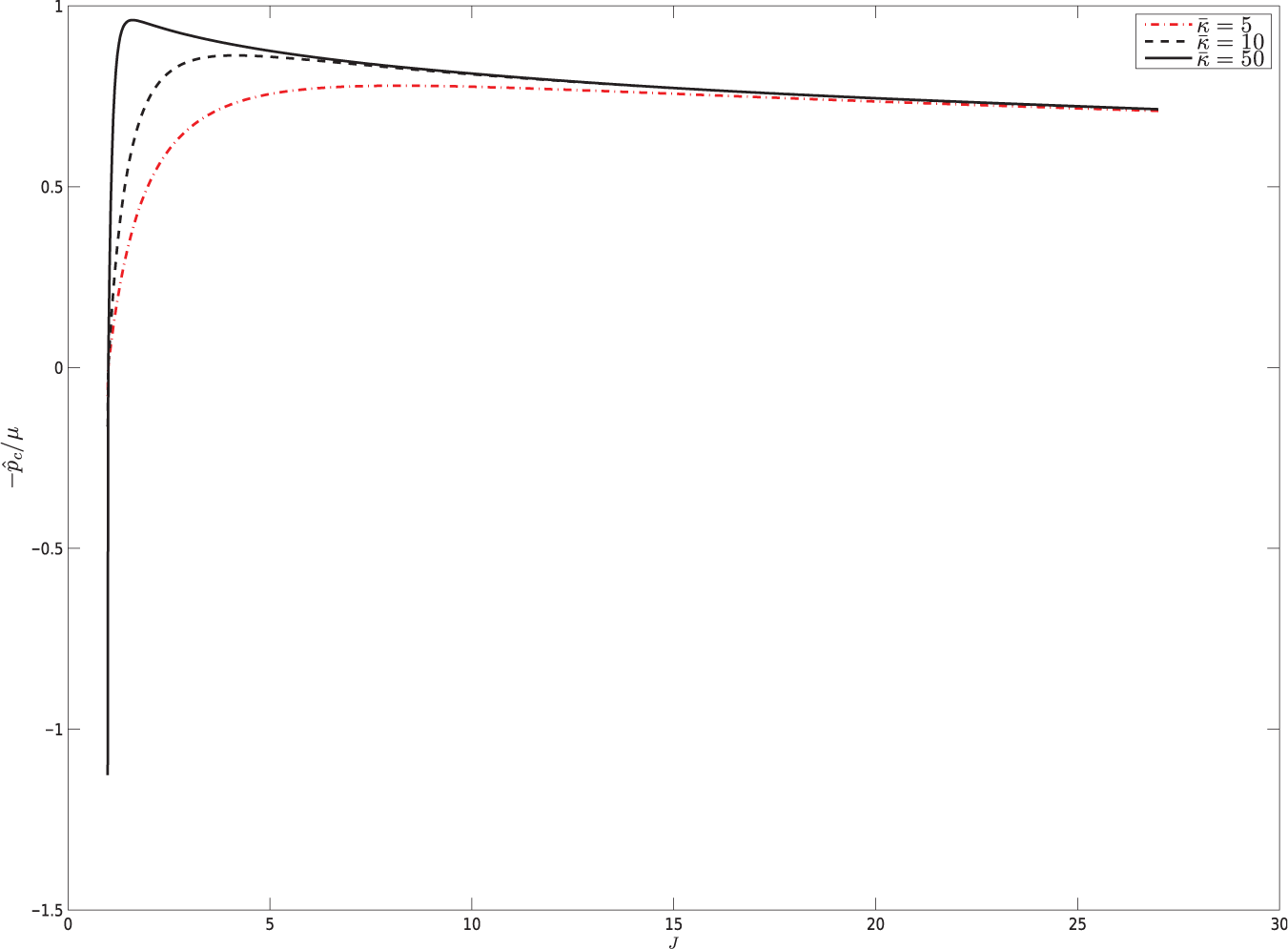
Thus, as κ→∞ the graph of the functions $- {\hat{p}}_{a} (J)$ and $- {\hat{p}}_{b} (J)$ tend to that of a vertical line at J = 1. In contrast, the graph of $- {\hat{p}}_{c} (J)$ tends to a graph that consists of two parts that connect to each other at J = 1, $- {\hat{p}}_{c} = μ$ . One part is a vertical ray with endpoint J = 1, $- {\hat{p}}_{c} = μ$ that then proceeds to $- {\hat{p}}_{c} = - \infty$ . The other part is a curve expressed by $- {\hat{p}}_{c} (J) = μ / J^{1 / 3}$ with starting point at J = 1, $- {\hat{p}}_{c} = μ$ (Figure 2).

Figure 2.

Plot of $- {\hat{p}}_{c} / μ$ versus J for pure pressure load at various $\bar{κ}$ = κ/μ. In the limit as κ → ∞ the curve tends to a two-part graph. The first part is a vertical line segment through J = 1 that ends at $- {\hat{p}}_{c} / μ$ = 1, and the second part is the monotonically decreasing function 1/J^1/3. The two parts connect at $- {\hat{p}}_{c} / μ$ = 1. The other two models W_a and W_b give a more conventional monotonic behavior that approaches the vertical line J = 1 as $\bar{κ}$ → ∞.

3. Energy contours

Consider the level curves of W(I₁, J) in the admissible region $D = {(I_{1}, J) : I_{1} \geq 3 J^{2 / 3}, J > 0}$ . Note that, for all three models W_a, W_b and W_c, the energy density continues to be defined on the full quadrant $Q = {(I_{1}, J) : I_{1} > 0, J > 0}$ . When discussing behavior near the boundary $\partial D$ of $D$ it is often useful to imagine continuing the curves of constant W out of $D$ while still in $Q$ . Specifically, it is useful to describe the way in which the level curves “cut” $\partial D$ .

Recall that $\partial D$ corresponds to F = J^1/3I and, hence, pressure loading. Let $\partial D^{+}$ and $\partial D^{-}$ correspond respectively to the J ≥ 1 and J ≤ 1 parts of $\partial D$ . The intersection of these two parts is the point (I₁, J) = (3,1) corresponding to the reference state. All three energy densities W_a, W_b and W_c have been constructed such that the reference configuration point (I₁, J) = (3, 1) gives W = 0.

For all three models W_a, W_b and W_c it follows that W increases with J on the boundary portion $\partial D^{+}$ . This is an immediate consequence of (2.6) because all three functions ${\hat{p}}_{a} (J)$ , ${\hat{p}}_{b} (J)$ , and ${\hat{p}}_{c} (J)$ are negative for J>1. Similarly, because all three functions ${\hat{p}}_{a} (J)$ , ${\hat{p}}_{b} (J)$ and ${\hat{p}}_{c} (J)$ are positive for J < 1, it follows from (2.6) that all of these W functions increase as J decreases on the boundary portion $\partial D^{-}$ . In particular, on $\partial D$ it follows that

W_{a} (3 J^{2 / 3}, J) = \frac{3 μ}{2} (J^{2 / 3} - 1) + (\frac{κ}{2} - \frac{μ}{3}) {(J - 1)}^{2} - μ ln J,

(3.1)

and

W_{b} (3 J^{2 / 3}, J) = \frac{κ}{8} (J^{2} + \frac{1}{J^{2}} - 2),

(3.2)

and

W_{c} (3 J^{2 / 3}, J) = \frac{3 μ}{2} (J^{2 / 3} - 1) + \frac{3 μ^{2}}{3 κ - 2 μ} (J^{\frac{2}{3} - \frac{κ}{μ}} - 1) .

(3.3)

Thus, as J→∞ on $\partial D$ all three model energy functions W_a, W_b and W_c tend to infinity. Also, as J→ 0 on $\partial D$ all three model energy functions W_a, W_b and W_c again tend to infinity.

Consider W_a(I₁, J). Then for any fixed number w>0 there exists a unique location on $\partial D^{+}$ such that W_a = w. Similarly there exists a unique location on $\partial D^{-}$ such that W_a = w. This permits the definition of functions ${\hat{J}}_{\partial D^{+}}^{(a)} (w)$ and ${\hat{J}}_{\partial D^{-}}^{(a)} (w)$ obeying ${\hat{J}}_{\partial D^{+}}^{(a)} (w) > 1$ and $0 < {\hat{J}}_{\partial D^{-}}^{(a)} (w) < 1$ such that $J = {\hat{J}}_{\partial D^{+}}^{(a)} (w)$ locates the position on $\partial D^{+}$ where W_a = w and $J = {\hat{J}}_{\partial D^{-}}^{(a)} (w)$ locates the position on $\partial D^{-}$ where W_a = w. The following characterization of the level sets of energy is then immediate:

The locus of $(I_{1}, J) \in D$ making W_a(I₁, J) = w is a single-level curve with one endpoint on $\partial D^{+}$ as located by $J = {\hat{J}}_{\partial D^{+}}^{(a)} (w)$ and the other endpoint on $\partial D^{-}$ as located by $J = {\hat{J}}_{\partial D^{-}}^{(a)} (w)$ . There exists a function ${\hat{I}}_{1}^{(a)} (J, w)$ defined on ${(J, w) : w > 0, {\hat{J}}_{\partial D^{-}}^{(a)} (w) \leq J \leq {\hat{J}}_{\partial D^{+}}^{(a)} (w)}$ such that this level curve is given by

I_{1} = {\hat{I}}_{1}^{(a)} (J, w) for {\hat{J}}_{\partial D^{-}}^{(a)} (w) \leq J \leq {\hat{J}}_{\partial D^{+}}^{(a)} (w) (level set W_{a} (I_{1}, J) = w) .

(3.4)

Proof. Fix w>0 and $J \in [{\hat{J}}_{\partial D^{-}}^{(a)} (w), {\hat{J}}_{\partial D^{+}}^{(a)} (w)]$ . The value of J then locates a unique point $(I_{1}, J) = (3 J^{2 / 3}, J) \in \partial D$ . At this point W_a ≤ w with equality only if J corresponds to one of the endpoints, either $J = {\hat{J}}_{\partial D^{-}}^{(a)} (w)$ or $J = {\hat{J}}_{\partial D^{+}}^{(a)} (w)$ . Now consider a horizontal path in $D$ beginning from $\partial D$ . It follows from (2.11) that W_a(I₁, J) →∞ as I₁→∞. Thus, by continuity, there exists one or more roots I₁ to the equation W_a(I₁, J) = w for I₁ ≥ 3J^2/3. W_a is monotonically increasing with respect to I₁ since ∂W_a/∂I₁>0 and hence any such root is unique. This unique root defines the value of the function ${\hat{I}}_{1}^{(a)} (J, w)$ .

Corresponding results apply for the models W_b(I₁, J) and W_c(I₁, J). In particular, there exists a function ${\hat{I}}_{1}^{(b)} (J, w)$ such that the locus W_b(I₁, J) = w>0 is described by $I_{1} = {\hat{I}}_{1}^{(b)} (J, w)$ on the appropriate J-interval (which is again determined by the level set endpoints on $\partial D$ ). A corresponding function ${\hat{I}}_{1}^{(c)} (J, w)$ also exists for describing the locus W_c(I₁, J) = w>0.□

Of interest is the slope of the level set curves in the (I₁, J)-plane. Differentiation of W(I₁, J) = w gives

\frac{dJ}{{dI}_{1}} = - \frac{\partial W}{\partial I_{1}} / \frac{\partial W}{\partial J} for the level set curve of W (I_{1}, J) = w .

(3.5)

We have here chosen to work with dJ/dI₁ because I₁ is the abscissa (horizontal axis) and J is the ordinate (vertical axis) in our (I₁, J)-diagrams. For the three model materials W_a, W_b, W_c the reciprocal of this slope, i.e. dI₁/dJ, is formally the partial derivative of the corresponding function ${\hat{I}}_{1}^{(a)} (J, w)$ , ${\hat{I}}_{1}^{(b)} (J, w)$ or ${\hat{I}}_{1}^{(c)} (J, w)$ whose existence has just been demonstrated.

Consider the level set for W(I₁, J) = 0. For W_a, W_b and W_c the previous considerations show that the intersection of this level set with $D$ consists of only the single reference configuration point (I₁, J) = (3, 1). This point is on $\partial D$ . However, the set W(I₁, J) = 0 will still continue into the quadrant $Q$ as a curve. More generally, the slope of the level set curve passing through the reference configuration point (I₁, J) = (3,1) can be evaluated from (3.5) using the stress-free reference configuration requirement (2.4). This gives dJ/dI₁ = 1/2. On the other hand, consider the slope of the curve $\partial D$ (which is not a level set curve) at (I₁, J) = (3,1). It follows from differentiation of (2.2) that the slope of the curve $\partial D$ is dJ/dI₁ = J^1/3/2. At (I₁, J) = (3,1) this slope evaluates to dJ/dI₁ = 1/2, the same value as the level set curve passing through that point. Thus the algebraic condition (2.4) has an immediate interpretation in terms of the geometry of the level set curves. Namely

The reference configuration is stress free if and only if the energy contour in $Q$ passing through the reference location point (I₁, J) = (3, 1) osculates the boundary $\partial D$ of the admissible region at that point.

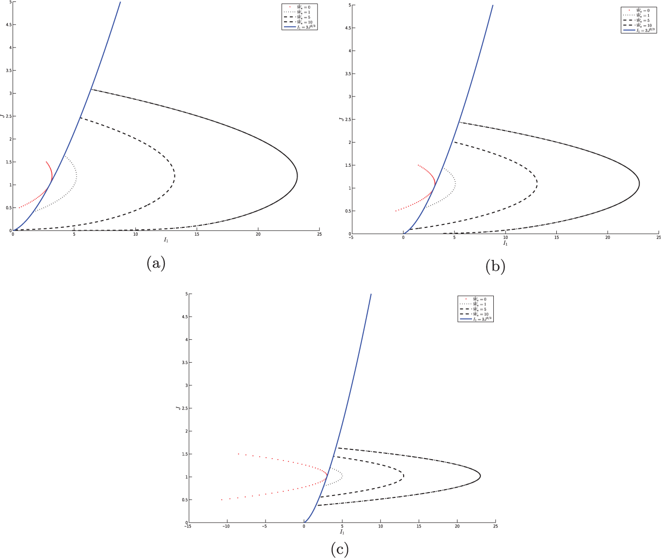
Figure 3 displays energy contours in the (I₁, J) plane for W_a. Each subfigure corresponds to a different value of κ using normalizations ${\bar{W}}_{a} = W_{a} / μ$ and $\bar{κ} = κ / μ$ . As required, for each $\bar{κ}$ the ${\bar{W}}_{a} = 0$ contour is tangent to the boundary $\partial D$ of the admissible region at the point (I₁, J) = (3, 1). For each fixed w>0 the contour ${\bar{W}}_{a} = w > 0$ begins on $\partial D^{-}$ at $J = {\hat{J}}_{\partial D^{-}}^{(a)} (w) < 1$ . As J increases the contour proceeds into $D$ such that I₁ increases as the contour continues through J = 1. It reaches a maximum I₁ value at $J = \frac{1}{2} (1 + \sqrt{(3 \bar{κ} + 10) / (3 \bar{κ} - 2)})$ . After this I₁ decreases with J as the contour returns to the $\partial D^{+}$ part of $\partial D$ at $J = {\hat{J}}_{\partial D^{+}}^{(a)} (w) > 1$ . For a fixed w>0 if one considers a sequence of increasing $\bar{κ}$ , then the corresponding sequence of ${\bar{W}}_{b} = w$ contours will narrow and approach points on the line segment {(I₁, J) : 3 ≤ I₁ ≤ 3 + 2w/μ, J = 1} in the limit as $\bar{κ} \to \infty$ . Note that the endpoint I₁ = 3 + 2w/μ causes this result to coincide with that of the neo-Hookean material (1.1).

Figure 3.

The (I₁, J) contours of normalized energy ${\bar{W}}_{a}$ = $W_{a} / μ$ for various $\bar{κ}$ = κ/μ (a) $\bar{κ}$ = 5; (b) $\bar{κ}$ = 10; (c) $\bar{κ}$ = 50. The contour ${\bar{W}}_{a}$ = 0 is tangent to the bound curve I₁=3J^2/3 at (I₁, J) = (3, 1). Each ${\bar{W}}_{a}$ contour has a maximum of I₁ and this maximum occurs at a common value of J that depends upon $\bar{κ}$ , but does not depend upon the value of ${\bar{W}}_{a}$ . Each fixed ${\bar{W}}_{a}$ contour narrows as $\bar{κ}$ increases such that the contour sequence collapses onto the incompressible ray J = 1 in the limit $\bar{κ}$ → ∞.

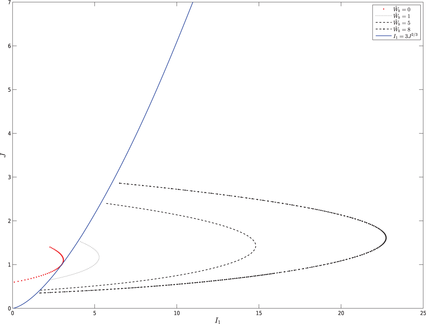
The form of the constant W_b contours is similar to those displayed for the W_a material as shown in Figure 4 for $\bar{κ} = 10$ . In particular, for each fixed w>0 the contour ${\bar{W}}_{b} = w > 0$ begins on $\partial D^{-}$ at $J = {\hat{J}}_{\partial D^{-}}^{(b)} (w) < 1$ . As J increases the contour proceeds into $D$ such that I₁ increases as the contour continues through J = 1. It again reaches a maximum I₁ value but now, unlike the W_a contours where the J corresponding to this I₁ maximum was the same for all w, the special J value that gives the I₁ maximum is found to vary with w. It is again found that these contours converge onto the line segment {(I₁, J) : 3 ≤ I₁ ≤ 3 + 2w/μ, J = 1} as $\bar{κ} \to \infty$ .

Figure 4.

The (I₁, J) contours of normalized energy ${\bar{W}}_{b}$ = W_b/μ for $\bar{κ}$ = 10. The form of the contours is similar to those for the W_a model (compare with Figure 3(b)).

Figure 5 shows the energy contours in the (I₁, J) plane for the energy W_c. The appearance of the fixed w>0 contours in this figure is different from those in Figures 3 and 4. Namely, after each such contour begins on $\partial D^{-}$ at $J = {\hat{J}}_{\partial D^{-}}^{(c)} (w) < 1$ one finds that this curve first proceeds at almost constant J for some range of I₁. It then experiences a rather abrupt turn so as to next proceed at almost constant I₁ as it returns to $\partial D$ at $J = {\hat{J}}_{\partial D^{+}}^{(c)} (w) > 1$ . This behavior becomes more pronounced for large $\bar{κ}$ . Unlike the constant energy contours for W_a and W_b one finds for W_c that I₁ is continuously increasing for all J. Hence, the maximum I₁ value on each constant W_c contour occurs at the endpoint with $J = {\hat{J}}_{\partial D^{+}}^{(c)} (w) > 1$ where the curve makes contact with $\partial D^{+}$ . For a fixed w > 0 if one considers a sequence of increasing $\bar{κ}$ then the corresponding sequence of W_c = w contours does not collapse onto a finite line segment {(I₁, J) : 3 ≤ I₁ ≤ 3 + 2w/μ, J = 1}. Instead the sequence of contours collapses onto a two-part curve. One part of this limiting curve is indeed the aforementioned horizontal line segment {(I₁, J) : 3 ≤ I₁ ≤ 3 + 2w/μ, J = 1}. However, the second part of this limiting curve is the vertical line segment {(I₁, J) : I₁ = 3 + 2w/μ, 1 ≤ J ≤ (1 + 2w/3μ)^3/2}.

Figure 5.

The (I₁, J) contours of normalized energy ${\bar{W}}_{c}$ = W_c/μ for various $\bar{κ}$ = κ/μ: (a) $\bar{κ}$ = 5; (b) $\bar{κ}$ = 10; (c) $\bar{κ}$ = 50. The contour ${\bar{W}}_{c}$ = 0 is tangent to the bound curve I₁=3J^2/3 at (I₁, J) = (3, 1). Each fixed ${\bar{W}}_{c}$ contour tends toward a two-part curve as $\bar{κ}$ increases: the first part collapses onto the incompressible ray J = 1 while the second part approaches a vertical line segment.

This last result may be understood by observing that (2.6) in conjunction with W(3, 1) = 0 indicates that the value of W on the boundary $\partial D$ is the area under the curve $- \hat{p} (J)$ between J = 1 and the J value for the point under consideration on $\partial D$ (this area is positive both for locations on $\partial D^{-}$ and for locations on $\partial D^{+}$ ). We recall that in the limit $\bar{κ} \to \infty$ the graphs of the functions $- {\hat{p}}_{a} (J)$ and $- {\hat{p}}_{b} (J)$ approach a vertical line at J = 1. For any J≠ 1 this causes the area under the $- \hat{p} (J)$ graph to approach infinity. Hence, the four functions ${\hat{J}}_{\partial D^{-}}^{(a)} (w)$ , ${\hat{J}}_{\partial D^{+}}^{(a)} (w)$ , ${\hat{J}}_{\partial D^{-}}^{(b)} (w)$ , ${\hat{J}}_{\partial D^{+}}^{(b)} (w)$ all approach J = 1 as $\bar{κ} \to \infty$ at fixed w. This in turn causes the $\partial D^{-}$ endpoints and the $\partial D^{+}$ endpoints of the constant W contours to collapse onto (I₁, J) = (3, 1) so as to squeeze the limiting contour onto the line J = 1. However, the same argument only partially applies to the W_c model because the graph of the function $- {\hat{p}}_{c} (J)$ only approaches the vertical line J = 1 for values J ≤ 1. The above argument therefore applies to values J < 1 on $\partial D$ which is $\partial D^{-}$ . This generates the horizontal portion {(I₁, J) : 3 ≤ I₁ ≤ 3 + 2w/μ, J = 1} of the two-part limiting constant W_c contour. However, because $- {\hat{p}}_{c} (J)$ approaches the function μ/J^1/3 for J>1 in the limit $\bar{κ} \to \infty$ it is no longer the case that the $\partial D^{+}$ endpoint approaches J = 1 in this limit. Instead a separate analysis based on the area under the curve μ/J^1/3 shows that this will generate the vertical part of the limiting contour {(I₁, J) : I₁ = 3 + 2w/μ,1 ≤ J ≤ (1 + 2w/3μ)^3/2}.

The above considerations show that the constant W contours (or, equivalently, level set curves) for W_a and W_b have similar convergence properties in the limit $\bar{κ} \to \infty$ while a different qualitative convergence ensues for the W_c model. It is therefore interesting that for finite $\bar{κ}$ the W_a and W_c models give the same slope behavior on J = 1 while the W_b model gives a different slope behavior. Namely, if one considers the slope of the constant W contours as they cross the ray J = 1 one finds from (3.5) that

\frac{dJ}{{dI}_{1}} = \frac{1}{2} for each level set curve of W_{a} and W_{c} as it crosses J = 1 .

(3.6)

For material model W_b it follows from (3.5) that

\frac{dJ}{{dI}_{1}} = \frac{3}{2 I_{1}} for each level set curve of W_{b} as it crosses J = 1 .

(3.7)

Hence, like the W_a and W_c contours, the W_b contour has the required stress-free slope value 1/2 at the reference configuration point (I₁, J) = (3, 1). However, while the W_a and W_c contours maintain this value as I₁ increases on J = 1, for the W_b contours the slope value decreases monotonically to zero as I₁ increases on J = 1.

4. Uniaxial loading

Consider uniaxial loading in the e₁ direction so that the Cauchy stress tensor is

T = T_{uni} e_{1} \otimes e_{1} .

(4.1)

By symmetry the stretches on the directions e₂ and e₃ are identical, i.e. λ₂ = λ₃, so that

F = λ_{1} e_{1} \otimes e_{1} + λ_{2} (e_{2} \otimes e_{2} + e_{3} \otimes e_{3}),

(4.2)

and

I_{1} = λ_{1}^{2} + 2 λ_{2}^{2}, J = λ_{1} λ_{2}^{2} .

(4.3)

4.1. Neo-Hookean response

For the neo-Hookean material (and incompressible materials in general) the requirement J = 1 gives

λ_{2} = λ_{1}^{- 1 / 2} (incompressible materials in general) .

(4.4)

Comparing diagonal entries of T as given by (4.1) and (1.2) it follows from (4.2) and (4.4) that

T_{uni} = μ λ_{1}^{2} - p_{reac}, (from e_{1} \cdot {Te}_{1}),

(4.5)

and

0 = \frac{μ}{λ_{1}} - p_{reac}, (from e_{2} \cdot {Te}_{2}) .

(4.6)

Eliminating p_reac gives the well-known uniaxial neo-Hookean response

T_{uni} = μ (λ_{1}^{2} - \frac{1}{λ_{1}}), (neo - Hookean material) .

(4.7)

For both compressible and incompressible isotropic hyperelasticity the Poisson’s ratio ν and Youngs modulus E can be obtained via

ν \equiv - {\frac{d λ_{2}}{d λ_{1}} |}_{λ_{1} = 1} and E \equiv {\frac{{dT}_{uni}}{d λ_{1}} |}_{λ_{1} = 1},

(4.8)

where it is presumed that T_uni is expressed as a function of stretch λ₁ alone. For the neo-Hookean material it therefore follows from these definitions in conjunction with (4.4) and (4.7) that ν = 1/2, the expected Poisson ratio for an incompressible material, and E = 3μ, the expected relation between Young and shear modulus for an incompressible material.

4.2. General compressible response

For the compressible models under consideration, comparison of the diagonal entries of T as given by (4.1) and (2.3) gives by virtue of (4.2) that

T_{uni} = \frac{2}{J} \frac{\partial W}{\partial I_{1}} λ_{1}^{2} + \frac{\partial W}{\partial J}, (from e_{1} \cdot {Te}_{1}),

(4.9)

and

0 = \frac{2}{J} \frac{\partial W}{\partial I_{1}} λ_{2}^{2} + \frac{\partial W}{\partial J}, (from e_{2} \cdot {Te}_{2}) .

(4.10)

In general, these are regarded as two equations relating T_uni, λ₁ and λ₂.

One may easily verify the previous claim that the standard formulae for the elastic constants ν and E now hold. To this end, implicit differentiation of (4.10) with respect to λ₁ gives

\begin{matrix} 0 = - \frac{2}{J^{2}} \frac{dJ}{d λ_{1}} \frac{\partial W}{\partial I_{1}} λ_{2}^{2} + \frac{2}{J} (\frac{\partial^{2} W}{\partial I_{1}^{2}} \frac{{dI}_{1}}{d λ_{1}} + \frac{\partial^{2} W}{\partial I_{1} \partial J} \frac{dJ}{d λ_{1}}) λ_{2}^{2} + \frac{4}{J} \frac{\partial W}{\partial I_{1}} λ_{2} \frac{d λ_{2}}{d λ_{1}} \\ + \frac{\partial^{2} W}{\partial I_{1} \partial J} \frac{{dI}_{1}}{d λ_{1}} + \frac{\partial^{2} W}{\partial J^{2}} \frac{dJ}{d λ_{1}} . \end{matrix}

(4.11)

This is to be evaluated at F = I where it is observed from (4.3) that

{\frac{{dI}_{1}}{d λ_{1}} |}_{F = I} = 2 - 4 ν, {\frac{dJ}{d λ_{1}} |}_{F = I} = 1 - 2 ν .

(4.12)

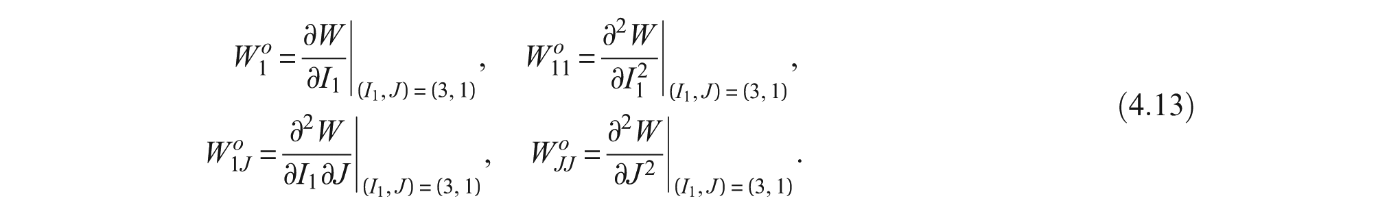
Here use has been made of the Poisson ratio definition in (4.8). We introduce the shorthand notation

\begin{matrix} W_{1}^{o} = {\frac{\partial W}{\partial I_{1}} |}_{(I_{1}, J) = (3, 1)}, W_{11}^{o} = {\frac{\partial^{2} W}{\partial I_{1}^{2}} |}_{(I_{1}, J) = (3, 1)}, \\ W_{1 J}^{o} = {\frac{\partial^{2} W}{\partial I_{1} \partial J} |}_{(I_{1}, J) = (3, 1)}, W_{JJ}^{o} = {\frac{\partial^{2} W}{\partial J^{2}} |}_{(I_{1}, J) = (3, 1)} . \end{matrix}

(4.13)

The evaluation of (4.11) at F = I yields

\begin{matrix} 0 = - 2 (1 - 2 ν) W_{1}^{o} + 2 ((2 - 4 ν) W_{11}^{o} + (1 - 2 ν) W_{1 J}^{o}) - 4 ν W_{1}^{o} + (2 - 4 ν) W_{1 J}^{o} + (1 - 2 ν) W_{JJ}^{o} \\ = - 2 W_{1}^{o} + (1 - 2 ν) (4 W_{11}^{o} + 4 W_{1 J}^{o} + W_{JJ}^{o}) . \end{matrix}

(4.14)

Solving this equation for ν gives

ν = \frac{- 2 W_{1}^{o} + 4 W_{11}^{o} + 4 W_{1 J}^{o} + W_{JJ}^{o}}{8 W_{11}^{o} + 8 W_{1 J}^{o} + 2 W_{JJ}^{o}} .

(4.15)

Simple manipulations using (2.7), (2.16) verifies the claim of Section 2.3 that

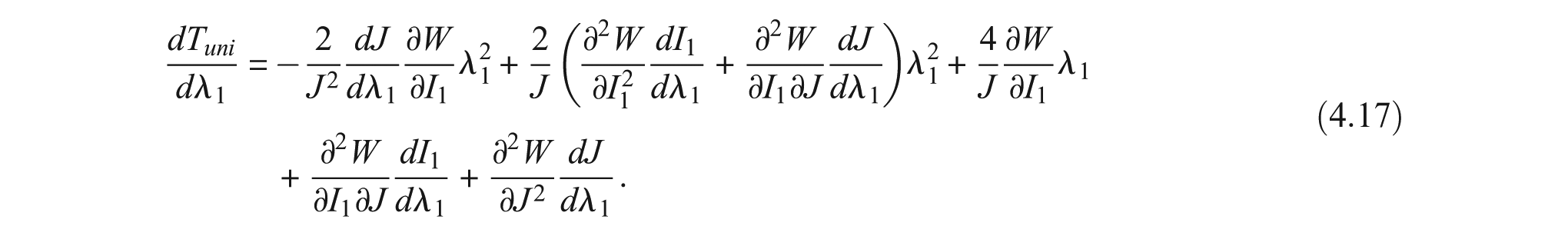
ν = \frac{(- 2 W_{1}^{o} + 12 W_{11}^{o} + 12 W_{1 J}^{o} + 3 W_{JJ}^{o}) - 4 W_{1}^{o}}{(- 4 W_{1}^{o} + 24 W_{11}^{o} + 24 W_{1 J}^{o} + 6 W_{JJ}^{o}) + 4 W_{1}^{o}} = \frac{3 κ - 2 μ}{6 κ + 2 μ} .

(4.16)

Turning to the determination of E, implicit differentiation of (4.9) with respect to λ₁ gives

\begin{matrix} \frac{{dT}_{uni}}{d λ_{1}} = - \frac{2}{J^{2}} \frac{dJ}{d λ_{1}} \frac{\partial W}{\partial I_{1}} λ_{1}^{2} + \frac{2}{J} (\frac{\partial^{2} W}{\partial I_{1}^{2}} \frac{{dI}_{1}}{d λ_{1}} + \frac{\partial^{2} W}{\partial I_{1} \partial J} \frac{dJ}{d λ_{1}}) λ_{1}^{2} + \frac{4}{J} \frac{\partial W}{\partial I_{1}} λ_{1} \\ + \frac{\partial^{2} W}{\partial I_{1} \partial J} \frac{{dI}_{1}}{d λ_{1}} + \frac{\partial^{2} W}{\partial J^{2}} \frac{dJ}{d λ_{1}} . \end{matrix}

(4.17)

Evaluation at F = I with the aid of (4.12) yields

{\frac{{dT}_{uni}}{d λ_{1}} |}_{λ_{1} = 1} = - 2 (1 - 2 ν) W_{1}^{o} + 2 ((2 - 4 ν) W_{11}^{o} + (1 - 2 ν) W_{1 J}^{o}) + 4 W_{1}^{o} + (2 - 4 ν) W_{1 J}^{o} + (1 - 2 ν) W_{JJ}^{o} .

(4.18)

Hence according to (4.8), E is given by

\begin{matrix} E = (2 + 4 ν) W_{1}^{o} + (4 - 8 ν) W_{11}^{o} + (4 - 8 ν) W_{1 J}^{o} + (1 - 2 ν) W_{JJ}^{o} \\ = 4 (1 + ν) W_{1}^{o} + \underset{zero by Equation (4.14)}{\underset{︸}{[- 2 W_{1}^{o} + (1 - 2 ν) (4 W_{11}^{o} + 4 W_{1 J}^{o} + W_{JJ}^{o})]}} = 2 (1 + ν) μ, \end{matrix}

(4.19)

where the last equality makes use of the definition of μ from (2.16). Eliminating ν between this result and (4.16) verifies the remaining Section 2.3 claim that E = 9κμ/(3κ + μ).

The above manipulations, which retrieve classical relations between the isotropic linear elastic constants for a W(I₁, J) hyperelastic material, indicate that as $\bar{κ} = κ / μ$ becomes large the uniaxial stress-stretch relations (4.9) and (4.10) for each of the material models W_a, W_b and W_c will be consistent with the incompressible theory in the small strain limit, and hence consistent with neo-Hookean behavior for small strains. Of more interest is the extent to which the uniaxial behavior for the W_a, W_b and W_c models tend to neo-Hookean behavior for finite strains as $\bar{κ}$ becomes large.

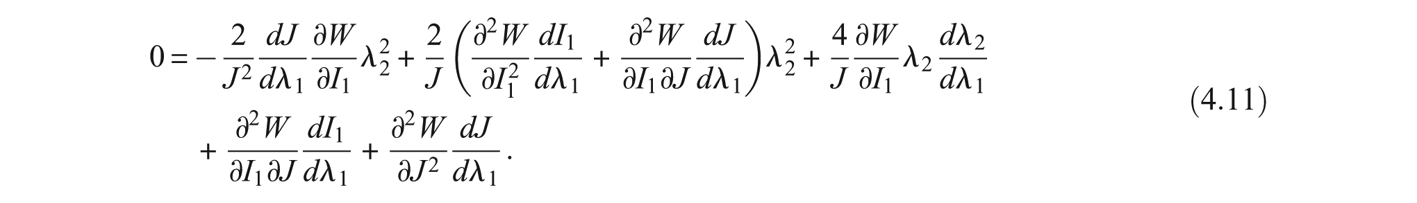
To this end we shall determine the nature of the uniaxial load paths in the (I₁, J)-plane for the different energy functions under consideration. As a preliminary result, suppose that λ₂ is locally a function of λ₁ in some portion of the uniaxial load curve. Then the slope dJ/dI₁ of the associated path in the (I₁, J)-plane is given by

\frac{dJ}{{dI}_{1}} = \frac{dJ / d λ_{1}}{{dI}_{1} / d λ_{1}} = \frac{\frac{d}{d λ_{1}} (λ_{1} λ_{2}^{2})}{\frac{d}{d λ_{1}} (λ_{1}^{2} + 2 λ_{2}^{2})} = \frac{λ_{2}^{2} + 2 λ_{1} λ_{2} \frac{d λ_{2}}{d λ_{1}}}{2 λ_{1} + 4 λ_{2} \frac{d λ_{2}}{d λ_{1}}} .

(4.20)

At the undeformed configuration value (I₁, J) = (3, 1) we have λ₁ = λ₂ = 1 and dλ₂/dλ₁ = −ν. Thus the above expression shows that each uniaxial load curve in the (I₁, J)-plane has slope dJ/dI₁ = 1/2 at (I₁, J) = (3, 1). This is the same slope value as that of the boundary curve $\partial D$ and as that of the level curve of energy W = 0 at (I₁, J) = (3, 1). Consequently, all three curves: the boundary curve $\partial D$ , energy contour W = 0, and uniaxial load curve, are mutually tangent to each other at (I₁, J) = (3, 1).

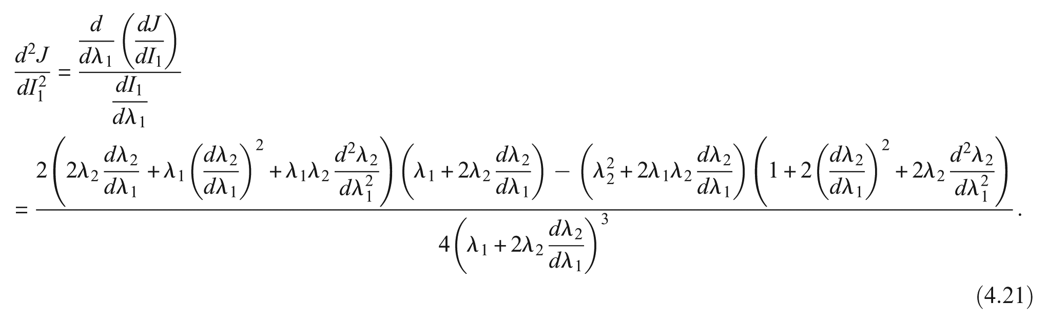
Now consider the second derivative of the uniaxial load curve in the (I₁, J)-plane. Again presuming that λ₂ is locally a function of λ₁ one may calculate

\begin{matrix} \frac{d^{2} J}{{dI}_{1}^{2}} = \frac{\frac{d}{d λ_{1}} (\frac{dJ}{{dI}_{1}})}{\frac{{dI}_{1}}{d λ_{1}}} \\ = \frac{2 (2 λ_{2} \frac{d λ_{2}}{d λ_{1}} + λ_{1} {(\frac{d λ_{2}}{d λ_{1}})}^{2} + λ_{1} λ_{2} \frac{d^{2} λ_{2}}{d λ_{1}^{2}}) (λ_{1} + 2 λ_{2} \frac{d λ_{2}}{d λ_{1}}) - (λ_{2}^{2} + 2 λ_{1} λ_{2} \frac{d λ_{2}}{d λ_{1}}) (1 + 2 {(\frac{d λ_{2}}{d λ_{1}})}^{2} + 2 λ_{2} \frac{d^{2} λ_{2}}{d λ_{1}^{2}})}{4 {(λ_{1} + 2 λ_{2} \frac{d λ_{2}}{d λ_{1}})}^{3}} . \end{matrix}

(4.21)

At the undeformed configuration value (I₁, J) = (3, 1) where λ₁ = λ₂ = 1 and dλ₂/dλ₁ = −ν the above result allows the second derivative to be written as

{\frac{d^{2} J}{{dI}_{1}^{2}} |}_{(I_{1}, J) = (3, 1)} = - \frac{1 + 4 ν}{4 {(1 - 2 ν)}^{2}} = \frac{1}{12} (1 - 9 {\bar{κ}}^{2}) .

(4.22)

It is notable that $d^{2} λ_{2} / d λ_{1}^{2}$ , which will generally depend upon the choice of W, cancels out of the expression (4.21) when λ₁ = λ₂ = 1. Hence, $d^{2} J / {dI}_{1}^{2}$ at the undeformed point (I₁, J) = (3, 1) is common for all models with the same κ/μ. Also $d^{2} J / {dI}_{1}^{2}$ at the undeformed point (I₁, J) = (3, 1) tends to ∞ in the incompressible limit $\bar{κ} \to \infty$ . This is consistent with the notion that all of these models should generate uniaxial load paths in the (I₁, J)-plane that in some way collapse onto the incompressible locus J = 1 in the incompressible limit. We now turn our attention to the qualitative nature of this collapse for the various models W_a, W_b and W_c under consideration.

4.3. Model W_a

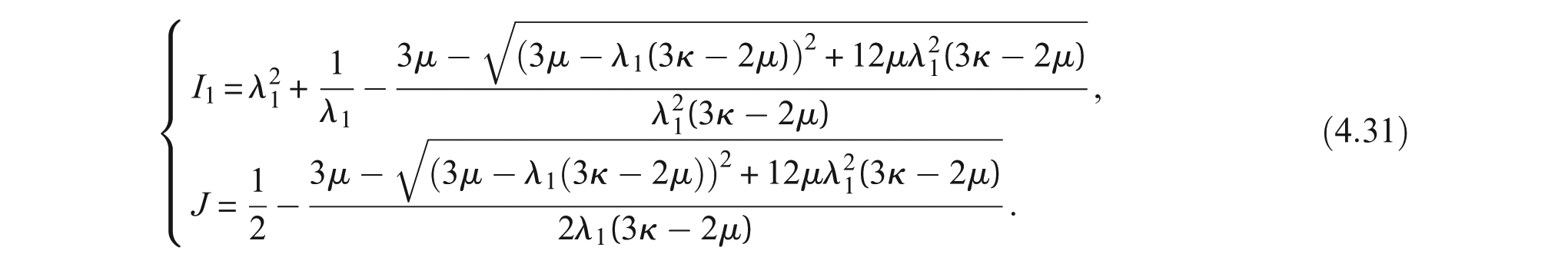
For W_a given by (2.11) the uniaxial load relations (4.9) and (4.10) specialize to

T_{uni} = \frac{μ}{λ_{2}^{2}} (λ_{1} - \frac{1}{λ_{1}}) + (κ - \frac{2}{3} μ) (λ_{1} λ_{2}^{2} - 1),

(4.23)

0 = \frac{μ}{λ_{1}} (1 - \frac{1}{λ_{2}^{2}}) + (κ - \frac{2}{3} μ) (λ_{1} λ_{2}^{2} - 1) .

(4.24)

The second of these determines the relation between λ₁ and λ₂. If κ = 2μ/3, then (4.24) gives the trivial solution λ₂ = 1 for all possible λ₁ (because κ = 2μ/3 this corresponds to ν = 0). If κ>2μ/3, then (4.24) can be expressed both as a quadratic equation in $λ_{2}^{2}$ and also as a quadratic equation in λ₁. When expressed as a quadratic equation in $λ_{2}^{2}$ it follows that both roots are real, however only one of these is positive for each λ₁>0. This leads to a unique determination of a single positive λ₂ for each positive λ₁. This unique determination is formally given by

λ_{2} = \sqrt{\frac{1}{2 λ_{1}} - \frac{1}{2 λ_{1}^{2} (3 \bar{κ} - 2)} (3 - \sqrt{{(3 - λ_{1} (3 \bar{κ} - 2))}^{2} + 12 λ_{1}^{2} (3 \bar{κ} - 2)})},

(4.25)

where again $\bar{κ} = κ / μ$ .

Consider the graph of λ₂ as a function of λ₁ for λ₁>0. Direct analysis of (4.25) shows that λ₂ as a function of λ₁ always involves

lim_{λ_{1} \to 0} λ_{2} = 1, lim_{λ_{1} \to \infty} λ_{2} = 0 .

(4.26)

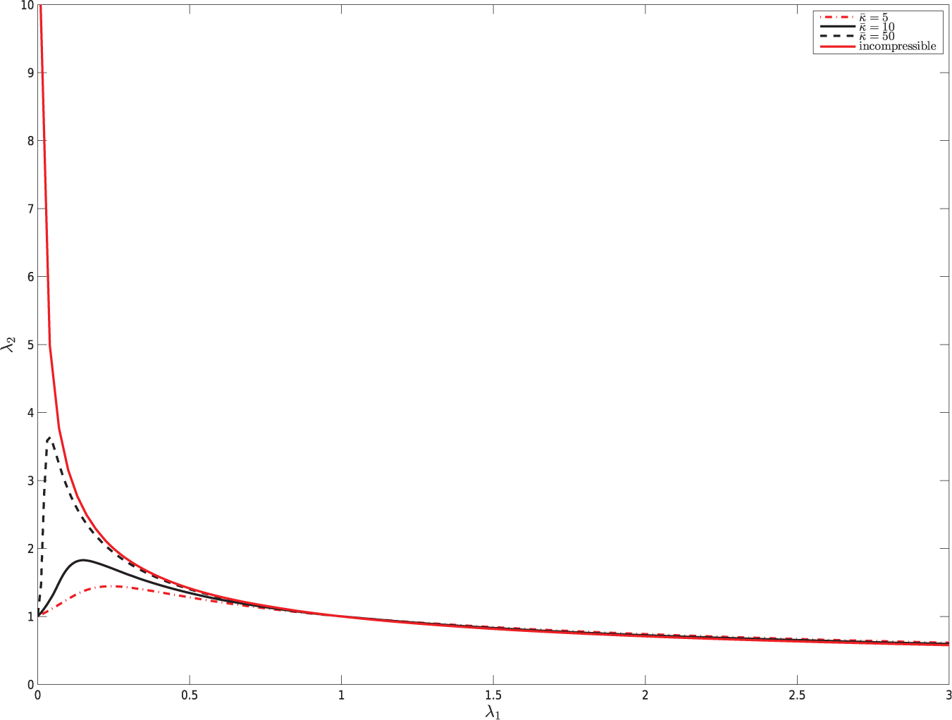
The graph of λ₂ as a function of λ₁ first increases from (λ₁, λ₂) = (0, 1) to a local maxima at

(λ_{1}, λ_{2}) = (\frac{6}{10 + 3 \bar{κ}}, \sqrt{\frac{5}{6} + \frac{1}{4} \bar{κ}}) .

(4.27)

The graph then monotonically decreases, passing through the requisite undeformed location (λ₁, λ₂) = (1, 1) before asymptoting to zero as λ₁→∞. Figure 6 shows plots of λ₂ versus λ₁ for various $\bar{κ}$ . The conspicuous feature is the anomalous behavior to the left of the global maximum $λ_{1} = 6 / (10 + 3 \bar{κ})$ where transverse and axial stretches decrease simultaneously. Note however that the value $λ_{1} = 6 / (10 + 3 \bar{κ})$ , which locates the local maximum, does proceed to zero as $\bar{κ} \to \infty$ . Moreover, in this limit of $\bar{κ} \to \infty$ it can be shown that the graph of λ₂ as a function of λ₁ approaches the incompressible result $λ_{2} = λ_{1}^{- 1 / 2}$ (pointwise, the convergence is nonuniform). At the undeformed location (λ₁, λ₂) = (1, 1) one verifies the requisite result $- d λ_{2} / d λ_{1} |_{λ_{1} = 1} = (3 \bar{κ} - 2) / 2 (3 \bar{κ} + 1) = ν$ and also obtains

(λ_{1}, λ_{2}) = (\frac{6}{10 + 3 \bar{κ}}, \sqrt{\frac{5}{6} + \frac{1}{4} \bar{κ}}) .

(4.28)

Figure 6.

Plot of λ₂ versus λ₁ for model Wa in uniaxial load with various $\bar{κ}$ = κ/μ. There is a local maximum at λ₁ = 6/(10 + $3 \bar{κ}$ ) and we note that this value of λ₁ tends to zero as $\bar{κ}$ becomes large. This causes the $\bar{κ}$ → ∞ limiting curve to converge onto the incompressible relation $λ_{2} = l / \sqrt{λ_{1}}$ , which is the solid red curve.

Turning to the Cauchy stress, together (4.23) and (4.25) permit T_uni to be formally written as a function of λ₁. One can verify that

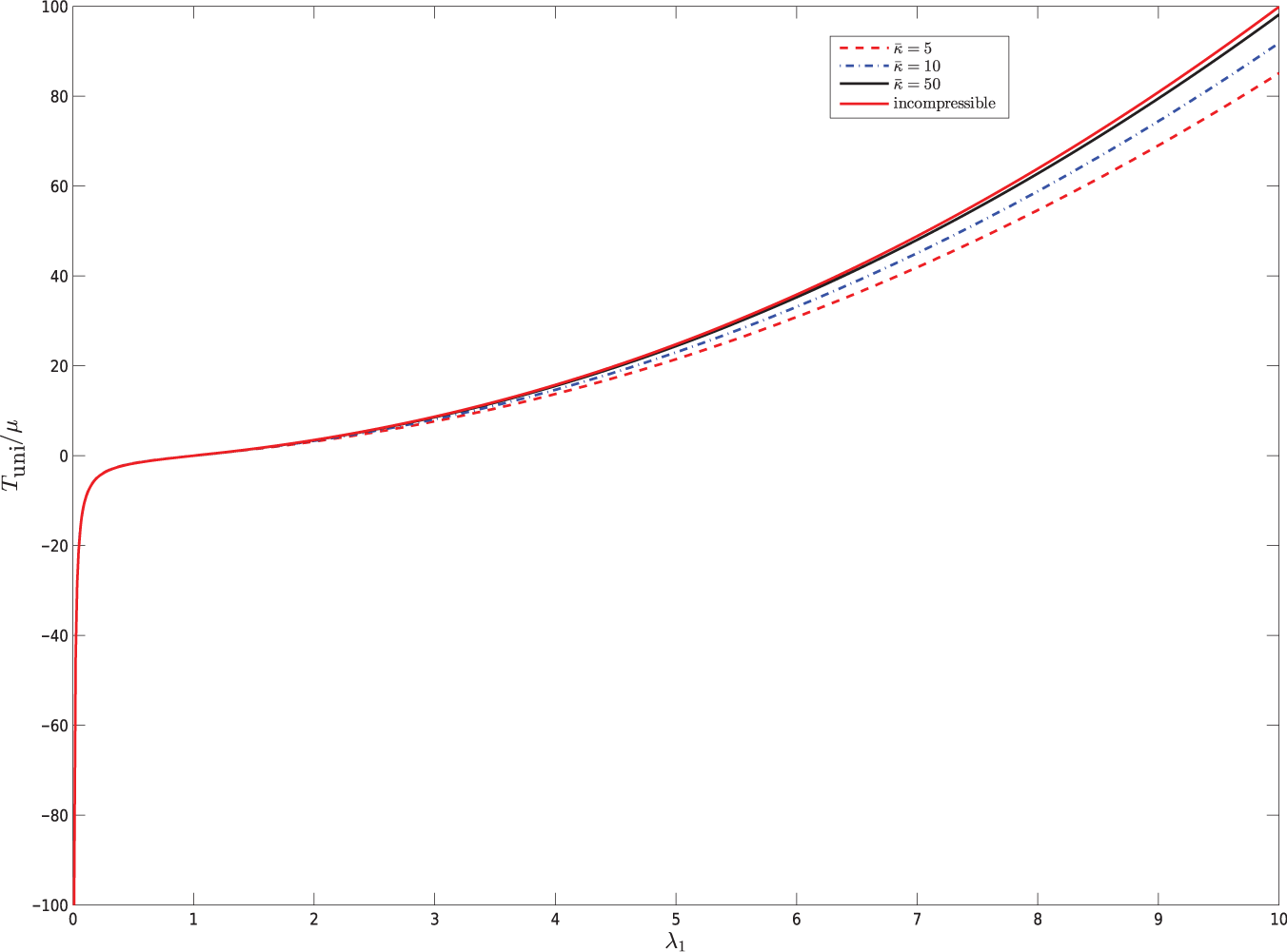
lim_{λ_{1} \to 0} T_{uni} = - \infty, lim_{λ_{1} \to \infty} T_{uni} = \infty .

(4.29)

Although the transverse stretch behavior was anomalous for $λ_{1} < 6 / (10 + 3 \bar{κ})$ , the stress T_uni exhibits conventional behavior in this regime. For example, one finds that

\frac{{dT}_{uni}}{d λ_{1}} |_{λ_{1} = \frac{6}{10 + 3 \bar{κ}}} = \frac{12 μ^{2}}{10 μ + 3 κ} + \frac{{(10 μ + 3 κ)}^{2}}{36 μ} > 0 .

(4.30)

More generally, T_uni as a function of λ₁ is found to be monotonically increasing (Figure 7). For any λ₁ it can be shown that there exists a sufficiently large $\bar{κ}$ so as to make T_uni (λ₁) as close as desired to the neo-Hookean value $μ (λ_{1}^{2} - 1 / λ_{1})$ . Hence, the uniaxial stretch-stress response for the W_a model approaches that of the neo-Hookean material in the limit $\bar{κ} \to \infty$ .

Figure 7.

Plot of T_uni/m versus λ₁ for model W_a with various $\bar{κ}$ . The uppermost curve is for the incompressible neo-Hookean material. For all cases, $\lim_{λ_{1} \to 0} T_{u n i} = - \infty$ and $\lim_{λ_{1} \to 0} T_{u n i} = \infty$ .

The uniaxial load path in the (I₁, J)-plane can be calculated parametrically using (4.3) and (4.25) with parameter λ₁ varying from 0 to ∞. Specifically,

{\begin{matrix} I_{1} = λ_{1}^{2} + \frac{1}{λ_{1}} - \frac{3 μ - \sqrt{{(3 μ - λ_{1} (3 κ - 2 μ))}^{2} + 12 μ λ_{1}^{2} (3 κ - 2 μ)}}{λ_{1}^{2} (3 κ - 2 μ)}, \\ J = \frac{1}{2} - \frac{3 μ - \sqrt{{(3 μ - λ_{1} (3 κ - 2 μ))}^{2} + 12 μ λ_{1}^{2} (3 κ - 2 μ)}}{2 λ_{1} (3 κ - 2 μ)} . \end{matrix}

(4.31)

It follows from these expressions that

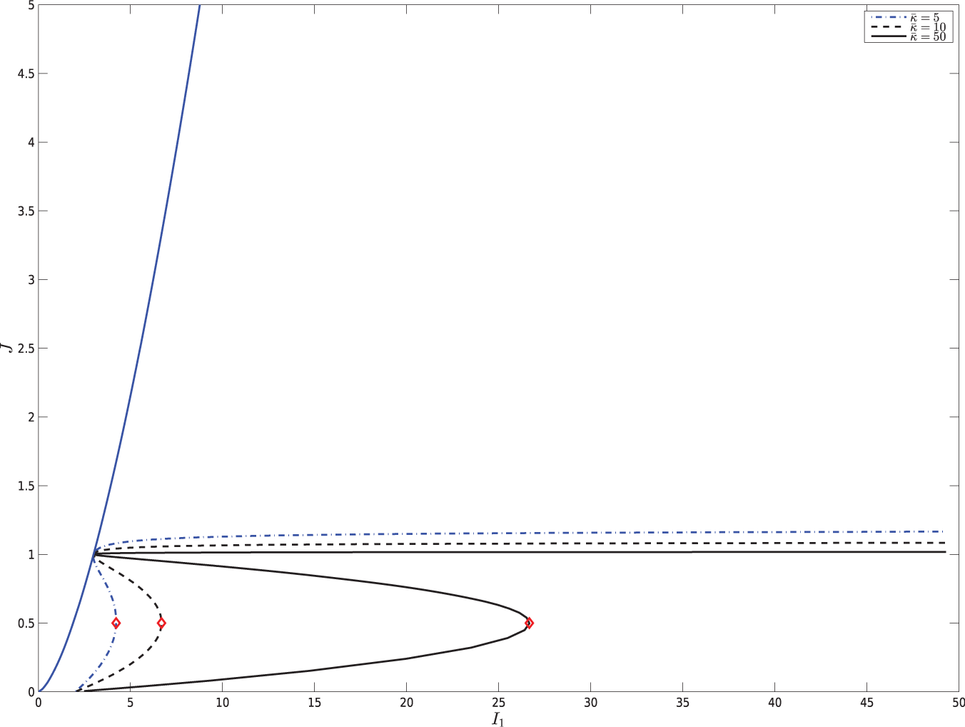
lim_{λ_{1} \to 0} (I_{1}, J) = (2, 0), lim_{λ_{1} \to \infty} (I_{1}, J) = (\infty, \frac{1}{2} + \frac{1}{2} \sqrt{1 + \frac{12 μ}{3 κ - 2 μ}}) .

(4.32)

The general form of the uniaxial load path in the (I₁, J)-plane is a curve with three distinguishable parts. The first part begins at (I₁, J) = (2, 0) such that both I₁ and J are then increasing to a local limit point value of I₁. The second part continues from this limit point value of I₁ and proceeds under increasing J to the undeformed point (I₁, J) = (3, 1). Then the third and final part continues from the undeformed point with both I₁ and J increasing. This third part asymptotes to

J = \frac{1}{2} + \frac{1}{2} \sqrt{1 + \frac{12}{3 \bar{κ} - 2}} > 1 as I_{1} \to \infty .

A sequence of such curves for various $\bar{κ}$ is shown in Figure 8. For general W these curves are tangent to the boundary $\partial D$ at the undeformed point (I₁, J) = (3, 1), i.e. dJ/dI₁ = 1/2 at this point.

Figure 8.

Uniaxial load paths in the (I₁, J)-plane with model W_a for various $\bar{κ}$ = κ/μ. Each curve has three distinguishable parts. The first (lowest) part begins at (I₁, J) = (2, 0) such that both I₁ and J are each increasing to a local limit point value of I₁. The second part continues from this limit point and proceeds under increasing J to the undeformed point (I₁, J) = (3, 1). The value of I₁ is generally decreasing on this part, but near the undeformed point the value of I₁ is increasing for a very small portion of this curve. Then the third and final part continues from the undeformed point with both I₁ and J increasing. This third part asymptotes to $J = \frac{l}{2} + \frac{l}{2} \sqrt{l + l 2 μ / (3 κ - 2 μ)} > 1$ as I₁→ ∞. The point in Figure 6 corresponding to the local maximum of the transverse stretch curve (red diamond) is very close to, but not at, the limit point.

Because

\frac{1}{2} + \frac{1}{2} \sqrt{1 + \frac{12}{3 \bar{κ} - 2}} \to 1 as \bar{κ} \to \infty,

it follows that the third (upper) part of the uniaxial load curve in the (I₁, J)-plane approaches the horizontal ray J = 1, I₁ ≥ 3 in the incompressible limit. We therefore turn our attention to the lower two parts of the uniaxial load curve in the (I₁, J)-plane.

Consider therefore the local limit point I₁ that separates the first and second parts of the uniaxial curve in the (I₁, J)-plane. By (4.3),

\frac{{dI}_{1}}{dJ} = \frac{\frac{{dI}_{1}}{d λ_{1}}}{\frac{dJ}{d λ_{1}}} = 0 \Rightarrow \frac{{dI}_{1}}{d λ_{1}} = 0 \Rightarrow 2 λ_{1} + 4 λ_{2} \frac{d λ_{2}}{d λ_{1}} = 0 \Rightarrow \frac{d λ_{2}}{d λ_{1}} = - \frac{λ_{1}}{2 λ_{2}} .

(4.33)

The last equality of (4.33) implies that the limit point that separates the first two parts of the uniaxial load curve in the (I₁, J)-plane corresponds to a λ₁ value that makes dλ₂/dλ₁ < 0.² Such a limit point λ₁ must therefore occur on the decreasing part of the transverse stretch curves (Figure 6). Thus, the λ₁ value associated with the limit point in Figure 8 obeys 6μ/(10μ + 3κ) < λ₁ < 1.

More importantly, as $\bar{κ} \to \infty$ the limit point value of I₁→∞ and this causes the lower and middle branches of the uniaxial load curve in the (I₁, J)-plane to approach separate limits. The lower branch approaches the horizontal ray J = 0, I₁ ≥ 2. The middle branch approaches the horizontal ray J = 1, I₁ ≥ 3. To be more precise, given any location on either of these rays and a specified neighborhood of that location there exists a sufficiently large $\bar{κ}$ so as to cause all uniaxial load curves with larger $\bar{κ}$ to pass through the neighborhood under consideration. On the other hand, given a value of λ₁ obeying 0 <λ₁ < 1 and any value of ϵ>0 there exists a value of $\bar{κ}$ such that all larger values of $\bar{κ}$ cause the corresponding value of (I₁, J) to be within an ϵ-neighborhood of the horizontal ray J = 1, I₁ ≥ 3. In this sense the uniaxial load paths in the (I₁, J)-plane converge onto the incompressible ray J = 1, I₁ ≥ 3 in the limit $\bar{κ} \to \infty$ .

4.4. Model W_b

For model W_b given by (2.12) the uniaxial load relations (4.9) and (4.10) specialize to

T_{uni} = \frac{μ λ_{1}^{1 / 3}}{λ_{2}^{10 / 3}} + \frac{κ}{4} (λ_{1} λ_{2}^{2} - \frac{1}{λ_{1}^{3} λ_{2}^{6}}) - \frac{μ (λ_{1}^{2} + 2 λ_{2}^{2})}{3 λ_{1}^{5 / 3} λ_{2}^{10 / 3}},

(4.34)

0 = \frac{μ}{λ_{1}^{5 / 3} λ_{2}^{4 / 3}} + \frac{κ}{4} (λ_{1} λ_{2}^{2} - \frac{1}{λ_{1}^{3} λ_{2}^{6}}) - \frac{μ (λ_{1}^{2} + 2 λ_{2}^{2})}{3 λ_{1}^{5 / 3} λ_{2}^{10 / 3}} .

(4.35)

Equation (4.35) neither gives an explicit analytical expression for λ₁ as a function of λ₂ nor does it give an analytical expression for λ₂ as a function of λ₁. Consequently we proceed with an implicit analysis.

Reorganize (4.35) into

\frac{κ}{4} λ_{2}^{8} - \frac{κ}{4 λ_{1}^{4}} - \frac{μ λ_{2}^{8 / 3}}{3 λ_{1}^{2 / 3}} + \frac{μ λ_{2}^{14 / 3}}{3 λ_{1}^{8 / 3}} = 0,

(4.36)

and consider the relation between λ₁ and λ₂ as $\bar{κ} = κ / μ \to \infty$ . To this end fix λ₁>0 and observe that ${lim}_{\bar{κ} \to \infty} λ_{2}$ is bounded. This follows because if λ₂→∞, then division of (4.36) by $κ λ_{2}^{8} / 4$ and subsequent consideration of $\bar{κ} \to \infty$ would lead to the contradiction 1 = 0. Now because both λ₁ and λ₂ are finite as $\bar{κ} \to \infty$ it follows from (4.36) that in this limit $λ_{2} \to 1 / \sqrt{λ_{1}}$ . Furthermore, a $\bar{κ} \to \infty$ dominant balance analysis of (4.36) under an assumption that $λ_{2} = λ_{1}^{- 1 / 2} + χ / {\bar{κ}}^{τ} + o (1 / {\bar{κ}}^{τ})$ with unknown constants χ and τ leads to

\frac{2 χ}{λ_{1}^{7 / 2} {\bar{κ}}^{τ - 1}} - \frac{1}{3 λ_{1}^{2}} - \frac{8 χ}{9 λ_{1}^{3 / 2} {\bar{κ}}^{τ}} + \frac{1}{3 λ_{1}^{5}} + \frac{14 χ}{9 λ_{1}^{9 / 2} {\bar{κ}}^{τ}} + h . o . t . = 0,

(4.37)

where h.o.t stands for higher-order terms. Consideration of the various balance possibilities leads to a conclusion that the three terms above the brackets in (4.37) provide the dominant balance with τ = 1. One then obtains that $χ = (λ_{1}^{3 / 2} - λ_{1}^{- 3 / 2}) / 6$ . Together this gives

λ_{2} = λ_{1}^{- 1 / 2} + \frac{λ_{1}^{3 / 2} - λ_{1}^{- 3 / 2}}{6 \bar{κ}} + o (\frac{1}{\bar{κ}}), for \bar{κ} = κ / μ \to \infty .

(4.38)

This in turn gives that

J = 1 + \frac{λ_{1}^{2} - λ_{1}^{- 1}}{3 \bar{κ}} + o (\frac{1}{\bar{κ}}), for \bar{κ} = κ / μ \to \infty

(4.39)

at fixed λ₁.

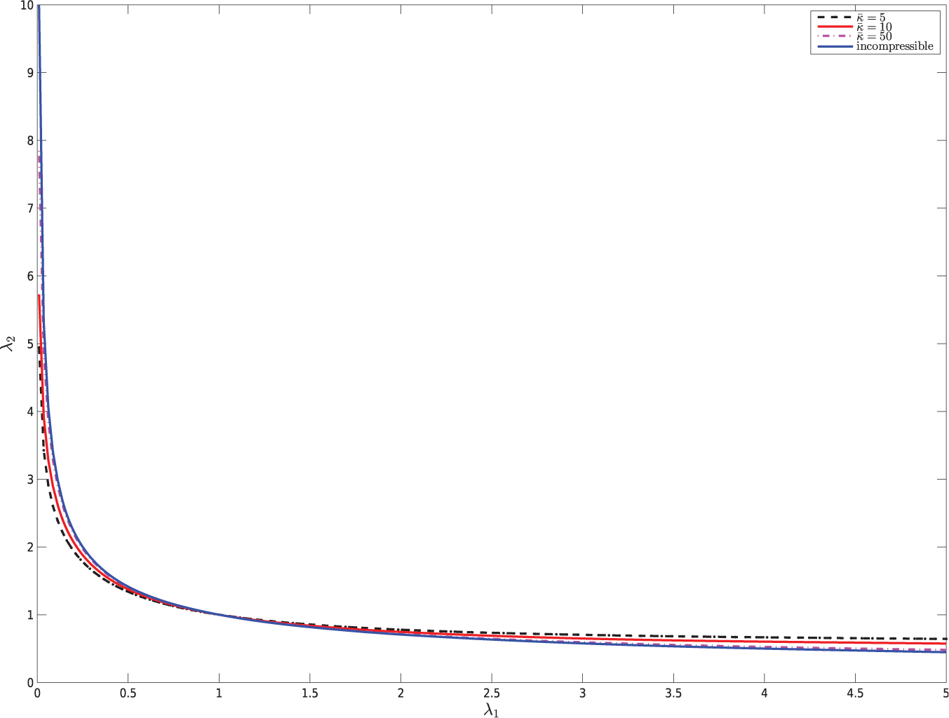
Having verified that $\bar{κ} \to \infty$ gives volume preservation and hence the incompressible limit we remark that this by itself does not preclude the possibility of an anomalous transverse stretch behavior for finite κ such as that which occurs for the W_a model (Figure 6). Numerical analysis however shows that such anomalous behavior does not occur (Figure 9).

Figure 9.

Plot of λ₂ versus λ₁ for model W_b in uniaxial load with various $\bar{κ}$ = κ/μ. The curve function is implicitly given by (4.35).

To establish such a result more definitively one may consider the separate limits of λ₁→ 0 and λ₁→∞ at finite $\bar{κ}$ . This is also useful for consideration of the uniaxial load curves in the (I₁, J)-plane for this material model. Consider first the limit λ₁→∞ in which case (4.36) gives

lim_{λ_{1} \to \infty} (- \frac{κ}{4 λ_{1}^{4}} - \frac{μ λ_{2}^{8 / 3}}{3 λ_{1}^{2 / 3}} + \frac{μ λ_{2}^{14 / 3}}{3 λ_{1}^{8 / 3}}) = - \frac{κ}{4} {(lim_{λ_{1} \to \infty} λ_{2})}^{8} \Rightarrow lim_{λ_{1} \to \infty} λ_{2} = 0 .

(4.40)

In particular, a λ₁→∞ dominant balance analysis of (4.36) under an assumption that $λ_{2} ~ ζ λ_{1}^{- η}$ with unknown constants ζ>0 and η>0 leads to

\frac{κ ζ^{8}}{4 λ_{1}^{8 η}} - \frac{κ}{4 λ_{1}^{4}} - \frac{μ ζ^{8 / 3}}{3 λ_{1}^{2 / 3 + 8 η / 3}} + \frac{μ ζ^{14 / 3}}{3 λ_{1}^{14 η / 3 + 8 / 3}} + h . o . t = 0 .

(4.41)

Consideration of the various balance possibilities leads to a conclusion that the two terms above the brackets in (4.41) provide the dominant balance with η = 1/8. One then obtains that ζ = (4μ/3κ)^3/16. Using this ζ and η, the next-order term in the expansion proceeds under the assumption that $λ_{2} ~ ζ λ_{1}^{- η} + ω λ_{1}^{- ρ}$ with unknown constants ω and ρ>1/8.

Thus, it is found that

λ_{2} = {(\frac{4 μ}{3 κ})}^{3 / 16} \frac{1}{λ_{1}^{1 / 8}} - \frac{3^{7 / 16}}{4^{23 / 16}} {(\frac{μ}{κ})}^{9 / 16} \frac{1}{λ_{1}^{19 / 8}} + o (\frac{1}{λ_{1}^{19 / 8}}) for λ_{1} \to \infty,

(4.42)

at fixed $\bar{κ} = κ / μ$ .

The limit λ₁→ 0 can be considered in a similar fashion wherein a dominant balance analysis yields

λ_{2} = {(\frac{3 κ}{4 μ})}^{3 / 14} \frac{1}{λ_{1}^{2 / 7}} - \frac{3}{14} {(\frac{3 κ}{4 μ})}^{27 / 14} λ_{1}^{10 / 7} + o (λ_{1}^{10 / 7}) for λ_{1} \to 0,

(4.43)

at fixed $\bar{κ} = κ / μ$ .

Turning next to the Cauchy stress component T_uni one obtains from (4.35) and (4.34) that

T_{uni} = μ (\frac{λ_{1}^{1 / 3}}{λ_{2}^{10 / 3}} - \frac{1}{λ_{1}^{5 / 3} λ_{2}^{4 / 3}}) .

(4.44)

Use of the expansion (4.38) in this result yields

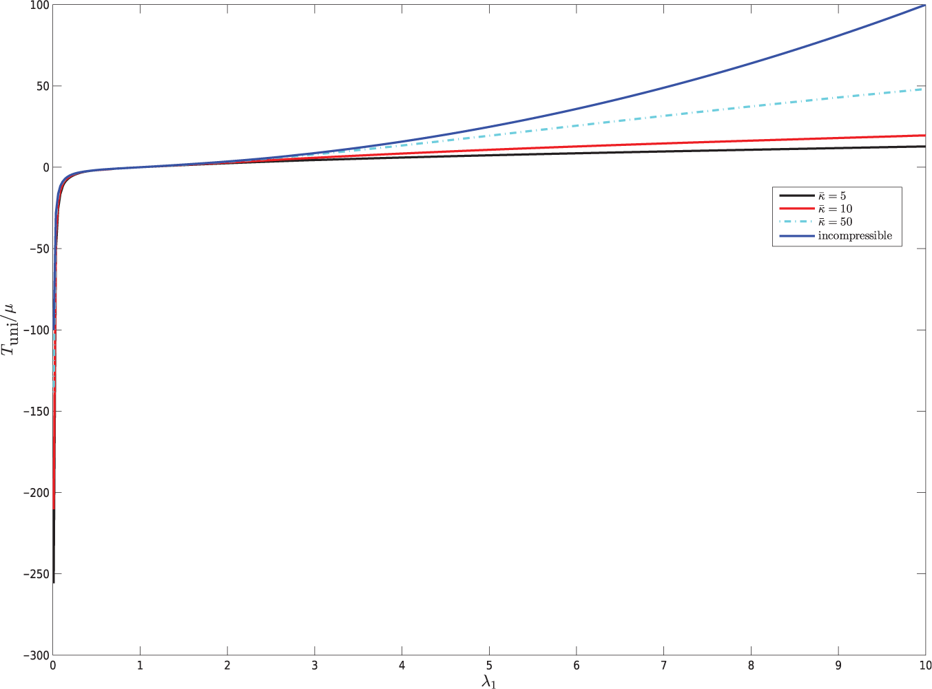
T_{uni} = μ (λ_{1}^{2} - \frac{1}{λ_{1}}) + \frac{μ (5 λ_{1}^{4} - 7 λ_{1} + 2 λ_{1}^{- 2})}{9 \bar{κ}} + o (\frac{1}{\bar{κ}}), for \bar{κ} = κ / μ \to \infty

(4.45)

at fixed λ₁. In particular, the neo-Hookean result is recovered in the limit $\bar{κ} \to \infty$ . Figure 10 displays the dependence of T_uni upon λ₁ for various $\bar{κ}$ . At fixed κ the asymptotic behavior of T_uni as λ₁→∞ follows from (4.44) in conjunction with (4.42). Similarly, at fixed κ the asymptotic behavior of T_uni as λ₁→ 0 follows from (4.44) in conjunction with (4.43). These give

T_{uni} = {\begin{matrix} μ {(\frac{3 κ}{4 μ})}^{5 / 8} λ_{1}^{3 / 4} + o (λ_{1}^{3 / 4}) for λ_{1} \to \infty, \\ - μ {(\frac{4 μ}{3 κ})}^{2 / 7} \frac{1}{λ_{1}^{9 / 7}} + o (\frac{1}{λ_{1}^{9 / 7}}) for λ_{1} \to 0 . \end{matrix}

(4.46)

Figure 10.

Plot of T_uni/μ versus λ₁ for model W_b with various $\bar{κ}$ . The uppermost curve is the incompressible neo-Hookean limit. For all cases, $\lim_{λ_{1} \to 0} T_{u n i} = - \infty$ and $\lim_{λ_{1} \to 0} T_{u n i} = \infty$ .

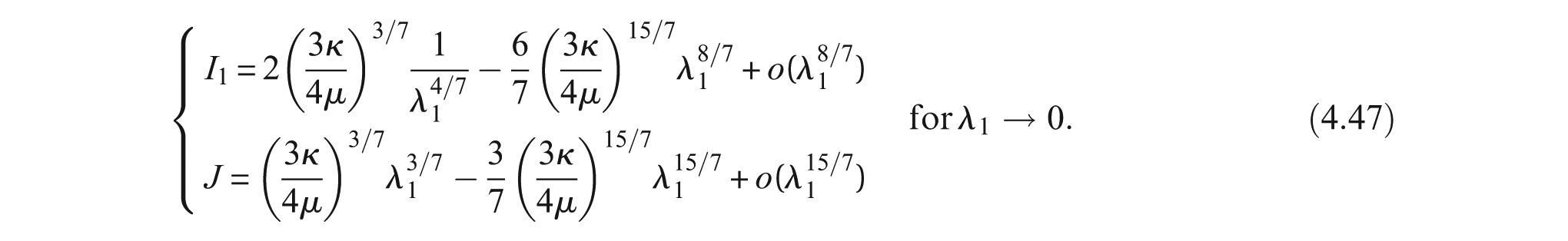
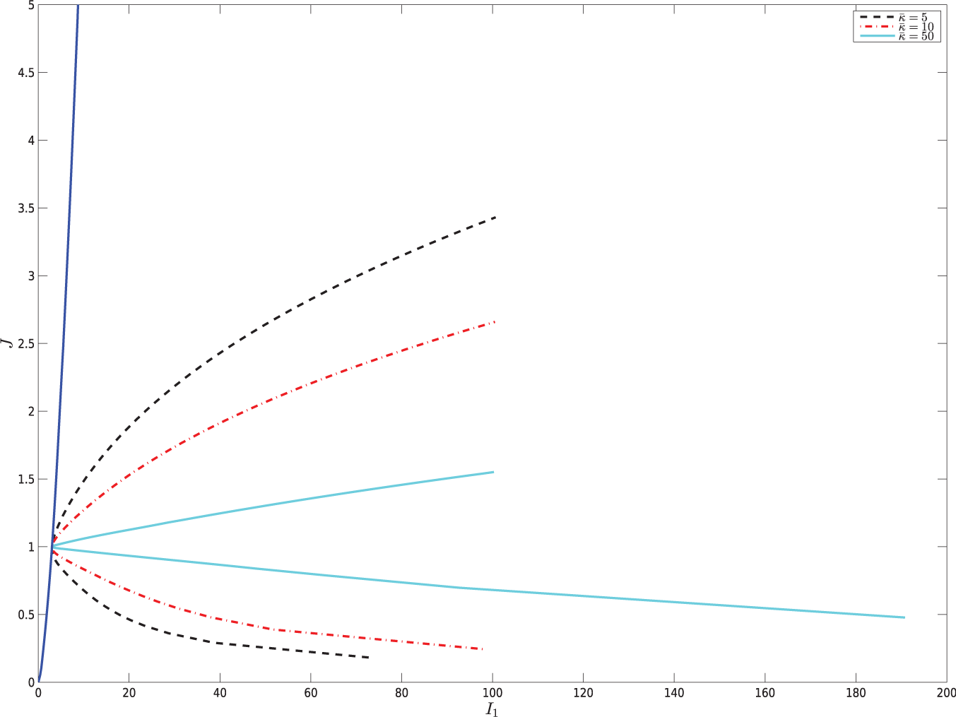
In particular, this confirms that ${lim}_{λ_{1} \to \infty} T_{uni} = \infty$ and ${lim}_{λ_{1} \to 0} T_{uni} = - \infty$ .

Consider now the uniaxial load paths in (I₁, J)-plane for this material. As is the case for the W_a model material, these paths for the W_b model material vary with $\bar{κ}$ . Figure 11 shows this variation. By virtue of (4.38) these curves collapse onto the horizontal ray J = 1, I₁ ≥ 3 as $\bar{κ} \to \infty$ . To be precise, given a value of λ₁>0 and any value of ϵ>0 there exists a value of $\bar{κ}$ such that all larger values of $\bar{κ}$ cause the corresponding value of (I₁,J) to be within an ϵ-neighborhood of the horizontal ray J = 1, I₁ ≥ 3. This is the same sense in which the previously considered W_a curves collapse onto the incompressible ray. However, unlike the W_a material, the W_b does not exhibit the limit point behavior on the λ₁ < 1 portion of the (I₁, J) path. In particular, at fixed $\bar{κ}$ the λ₁→ 0 limit of the (I₁, J) uniaxial load path is not a finite point in the (I₁,J)-plane as was the case for the W_a model. Rather, for the W_b material (4.43) gives

{\begin{matrix} I_{1} = 2 {(\frac{3 κ}{4 μ})}^{3 / 7} \frac{1}{λ_{1}^{4 / 7}} - \frac{6}{7} {(\frac{3 κ}{4 μ})}^{15 / 7} λ_{1}^{8 / 7} + o (λ_{1}^{8 / 7}) \\ J = {(\frac{3 κ}{4 μ})}^{3 / 7} λ_{1}^{3 / 7} - \frac{3}{7} {(\frac{3 κ}{4 μ})}^{15 / 7} λ_{1}^{15 / 7} + o (λ_{1}^{15 / 7}) \end{matrix} for λ_{1} \to 0 .

(4.47)

Figure 11.

Uniaxial load paths in the (I₁, J)-plane with model W_b for various $\bar{κ}$ . There is a single λ₁ < 1 branch and on this branch J→ 0 as I₁→ ∞. There is also a single λ₁ < 1 branch and on this branch J→ ∞ as I₁→ ∞. As $\bar{κ}$ → ∞, the contours all approach the incompressible ray J = 1, I₁ ≥ 3.

In particular, at fixed $\bar{κ}$ there is a single λ₁ < 1 branch to the uniaxial load curve in the (I₁, J)-plane, and as λ₁→ 0 this curve gives J→ 0 as I₁→∞.

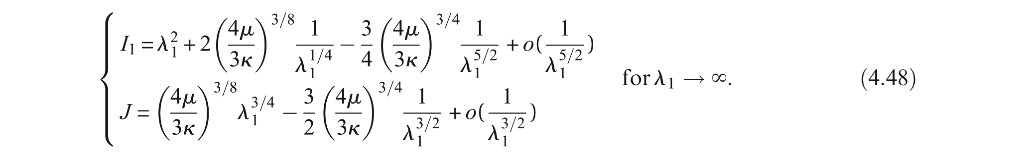
For λ₁>1 the W_b material gives a uniaxial load curve in the (I₁, J)-plane with a single branch. This is also the case for the W_a material. However, here it is to be recalled that the W_a material at fixed $\bar{κ}$ gives a finite J asymptote as λ₁→∞. This is not the case for the W_b model. Specifically (4.42) gives

{\begin{matrix} I_{1} = λ_{1}^{2} + 2 {(\frac{4 μ}{3 κ})}^{3 / 8} \frac{1}{λ_{1}^{1 / 4}} - \frac{3}{4} {(\frac{4 μ}{3 κ})}^{3 / 4} \frac{1}{λ_{1}^{5 / 2}} + o (\frac{1}{λ_{1}^{5 / 2}}) \\ J = {(\frac{4 μ}{3 κ})}^{3 / 8} λ_{1}^{3 / 4} - \frac{3}{2} {(\frac{4 μ}{3 κ})}^{3 / 4} \frac{1}{λ_{1}^{3 / 2}} + o (\frac{1}{λ_{1}^{3 / 2}}) \end{matrix} for λ_{1} \to \infty .

(4.48)

In particular, for the W_b material the upper branch of the uniaxial load curve gives J→∞ as I₁→∞.

Thus, both the W_a and W_b material models give uniaxial load curves in the (I₁, J)-plane that approach the requisite incompressible ray J = 1, I₁ ≥ 3 as $\bar{κ} \to \infty$ . However, the nature of the curves for finite $\bar{κ}$ has been shown to be qualitatively quite different.

4.5. Model W_c

For W_c given by (2.13) the uniaxial load relations (4.9) and (4.10) specialize to

T_{uni} = μ (\frac{λ_{1}}{λ_{2}^{2}} - \frac{1}{{(λ_{1} λ_{2}^{2})}^{\bar{κ} + 1 / 3}}),

(4.49)

0 = μ (\frac{1}{λ_{1}} - \frac{1}{{(λ_{1} λ_{2}^{2})}^{\bar{κ} + 1 / 3}}) .

(4.50)

The second of these gives the explicit relation

λ_{2} = λ_{1}^{- (3 \bar{κ} - 2) / (6 \bar{κ} + 2)},

(4.51)

which is monotonically decreasing and gives λ₂→ 0 as λ₁→∞ and also λ₂→∞ as λ₁→ 0 (a plot is omitted, the form would be similar to that of the W_b model in Figure 9). By (4.49) and (4.51),

T_{uni} = μ (λ_{1}^{(6 \bar{κ} - 1) / (3 \bar{κ} + 1)} - \frac{1}{λ_{1}}),

(4.52)

and the corresponding plot turns out to be very similar to that for the W_a model as previously displayed in Figure 7. Thus from (4.51) and (4.52), the incompressible neo-Hookean limits are immediate

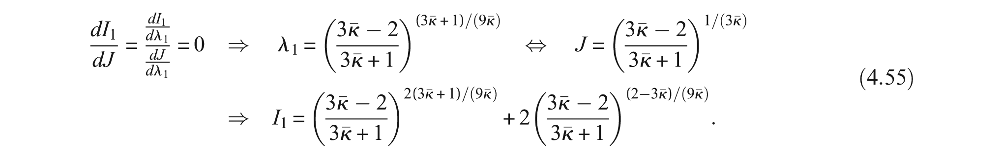
lim_{\bar{κ} \to + \infty} λ_{2} = \frac{1}{λ_{1}^{1 / 2}}, lim_{\bar{κ} \to + \infty} T_{uni} = μ (λ_{1}^{2} - \frac{1}{λ_{1}}) .

(4.53)

The relation between I₁ and J for the present case of uniaxial load is thus explicit for this material model

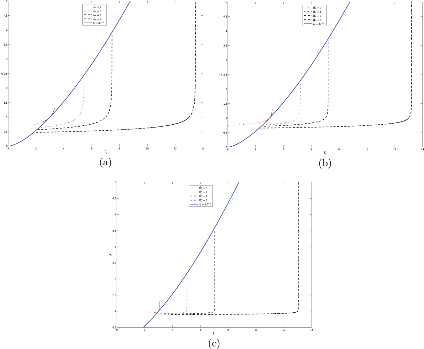
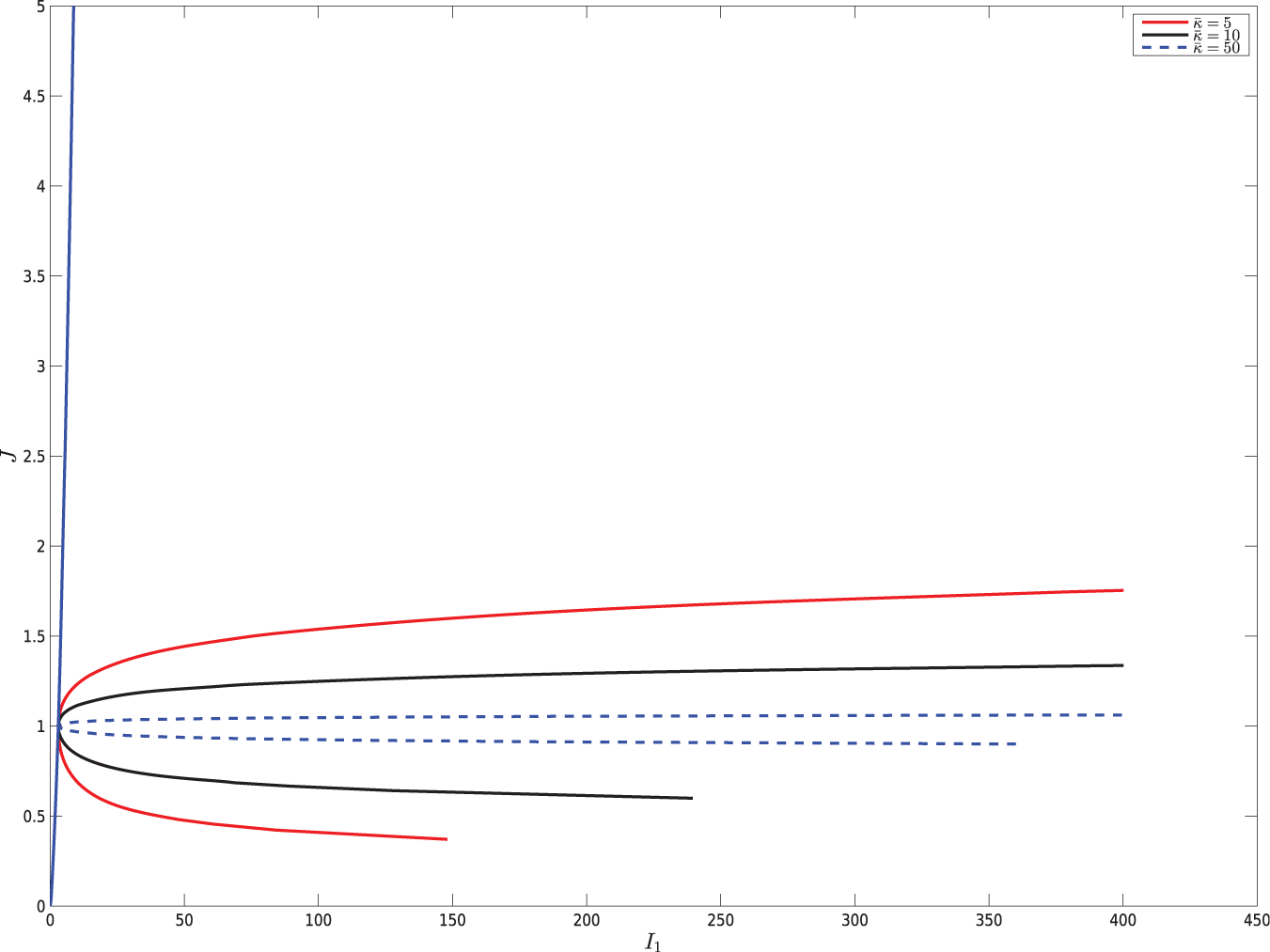
{\begin{matrix} I_{1} = λ_{1}^{2} + 2 λ_{1}^{- (3 \bar{κ} - 2) / (3 \bar{κ} + 1)} \\ J = λ_{1}^{3 / (3 \bar{κ} + 1)} \end{matrix} \Rightarrow I_{1} = J^{2 \bar{κ} + 2 / 3} + 2 J^{- \bar{κ} + 2 / 3} .

(4.54)

These contours are shown in Figure 12. As is the case for materials W_a and W_b these contours collapse onto the incompressible ray as $\bar{κ} \to \infty$ . At fixed finite $\bar{κ}$ each uniaxial load contour in the (I₁, J)-plane is qualitatively similar to those for the W_b material (but is qualitatively different from the three-branch result of the W_a material). Namely there is a single λ₁ < 1 branch and on this branch λ₁→ 0 gives I₁→∞ and J→ 0. There is similarly a single λ₁>1 branch and on this branch λ₁ → ∞ gives I₁→∞ and J → ∞.

Figure 12.

Uniaxial load paths in the (I₁, J)-plane with model Wc for various $\bar{κ}$ . There is a single λ₁ < 1 branch and on this branch J→ 0 as I₁→ ∞. There is also a single λ₁ < 1 branch and on this branch J→ ∞ as I₁ → ∞. As $\bar{κ}$ → ∞, the contours all approach the incompressible ray J = 1, I₁ ≥ 3.

Near the location corresponding to λ₁ = 1 the explicit nature of (4.54) permits an exact determination of the point on the λ₁ < 1 branch where I₁ is minimized. Namely

\begin{matrix} \frac{{dI}_{1}}{dJ} = \frac{\frac{{dI}_{1}}{d λ_{1}}}{\frac{dJ}{d λ_{1}}} = 0 \Rightarrow λ_{1} = {(\frac{3 \bar{κ} - 2}{3 \bar{κ} + 1})}^{(3 \bar{κ} + 1) / (9 \bar{κ})} \Leftrightarrow J = {(\frac{3 \bar{κ} - 2}{3 \bar{κ} + 1})}^{1 / (3 \bar{κ})} \\ \Rightarrow I_{1} = {(\frac{3 \bar{κ} - 2}{3 \bar{κ} + 1})}^{2 (3 \bar{κ} + 1) / (9 \bar{κ})} + 2 {(\frac{3 \bar{κ} - 2}{3 \bar{κ} + 1})}^{(2 - 3 \bar{κ}) / (9 \bar{κ})} . \end{matrix}

(4.55)

As required, in the limit as $\bar{κ} \to \infty$ the corresponding location in the (I₁, J)-plane converges onto (I₁, J) = (3, 1) which is the origination point of the incompressible ray.

5. Summary and discussion

The three different compressible hyperelastic models W_a(I₁,J), W_b(I₁,J) and W_c(I₁,J), which are respectively given by (2.11), (2.12) and (2.13), each provide a compressible version of the incompressible neo-Hookean material model. Each is endowed with a parameter κ such that the incompressible neo-Hookean behavior is obtained in an appropriate sense provided that κ≫μ. There are, however, certain qualitative differences in the nature of the approach to neo-Hookean behavior in the limit $\bar{κ} = κ / μ \to \infty$ . This was immediately apparent in the consideration of the pure pressure response. The pressure-volume response graph of an incompressible material is formally given by a vertical line. Indeed all three models W_a, W_b and W_c generate such a vertical line for positive pressures as $\bar{κ} \to \infty$ such that, prior to the limit, κ gives the slope of the graph at zero pressure. However, for negative (tensile) pressures it is only models W_a and W_b that continue to give the vertical line in the limit as $\bar{κ} \to \infty$ . The differing limiting (tensile) pressure response behavior for the W_c model can in turn be connected to the qualitatively different form of the constant energy contours in the (I₁, J)-plane. This can be seen by noting the similarity of the W_a and W_b contours (Figures 3 and 4) and their dissimilarity to the W_c contours (Figure 5).

While the W_c model gives anomalous behavior as regards pressure-volume response for tensile pressures, the W_a material model at finite κ (no matter how large) has an idiosyncratic transverse stretch behavior in uniaxial load. Namely, while the Cauchy stress–axial stretch response for the W_a model is properly monotonic for all values of axial stretch, there is always a regime of extreme axial stretch contraction in which the transverse stretch reverses direction from being elongational to being contractile. The W_a model still gives neo-Hookean behavior in the large κ limit, because the axial stretch interval that gives rise to this anomalous behavior becomes vanishingly small as κ→∞. Nevertheless, such an interval of anomalous behavior is always present for finite κ.

The above considerations might argue for the superiority of the W_b model. Here, however, it is to be pointed out that the W_b model delivers a different nonzero normal stress in simple shear than is exhibited by the W_a and W_c models. While it is arguable which nonzero normal stress is preferable (recall that all normal stresses cannot vanish in simple shear) the fact that W_a and W_c provide the same nonvanishing component, while the W_b model provides a different nonvanishing component is at least an interesting observation (consistency with the neo-Hookean result is here provided by the freedom to choose p_reac). It is also to be remarked that certain conventionally posed numerical procedures seem to be more sensitive to possible instabilities when using the W_b model because of the dependence on I₁/J^2/3.

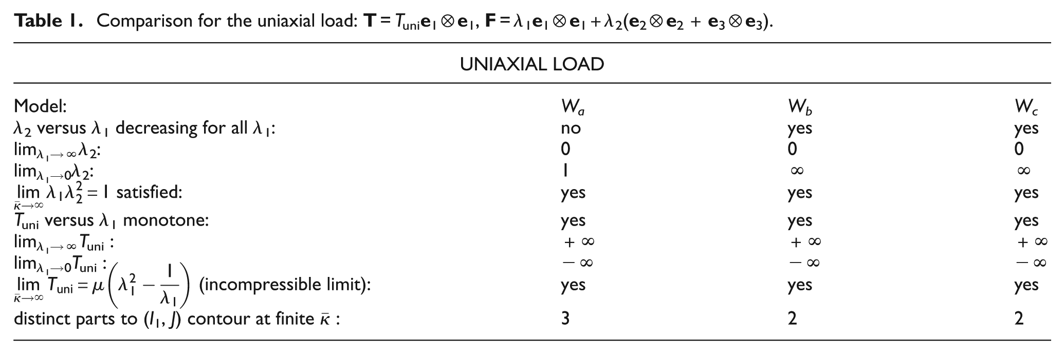
Table 1 summarizes the uniaxial loading response for the three model materials. Other states of load and deformation can be analyzed in a similar fashion. For example equibiaxial loading is characterized by F = λ₁(e₁⊗e₁ + e₂⊗e₂) +λ₃e₃⊗e₃ and T = T_bi (e₁⊗e₁ + e₂⊗e₂).

In this case (2.3) leads to

T_{bi} = e_{1} \cdot {Te}_{1} = \frac{2}{J} \frac{\partial W}{\partial I_{1}} λ_{1}^{2} + \frac{\partial W}{\partial J},

(5.1)

0 = e_{3} \cdot {Te}_{3} = \frac{2}{J} \frac{\partial W}{\partial I_{1}} λ_{3}^{2} + \frac{\partial W}{\partial J} .

(5.2)

Table 1.

Comparison for the uniaxial load: T = T_unie₁⊗e₁, F = λ₁e₁⊗e₁+λ₂(e₂⊗e₂ + e₃⊗e₃).

UNIAXIAL LOAD
Model:	W_a	W_b	W_c
λ₂ versus λ₁ decreasing for all λ₁:	no	yes	yes
lim_λ₁→∞λ₂:	0	0	0
lim_λ₁→0λ₂:	1	∞	∞
$\lim_{\bar{κ} \to \infty} λ_{1} λ_{2}^{2} = 1$ satisfied:	yes	yes	yes
T_uni versus λ₁ monotone:	yes	yes	yes
lim_λ₁→∞T_uni :	+∞	+∞	+∞
lim_λ₁→0T_uni :	−∞	−∞	−∞
$\lim_{\bar{κ} \to \infty} T_{uni} = μ (λ_{1}^{2} - \frac{1}{λ_{1}})$ (incompressible limit):	yes	yes	yes
distinct parts to (I₁, J) contour at finite $\bar{κ}$ :	3	2	2

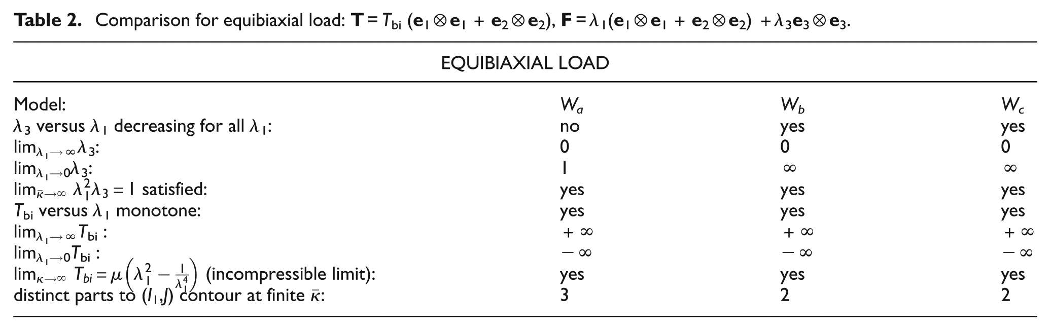
All three models give neo-Hookean behavior in an appropriate sense as $\bar{κ} \to \infty$ although the qualitative nature of the convergence is again material sensitive. The main results are summarized in Table 2.

Table 2.

Comparison for equibiaxial load: T = T_bi (e₁⊗e₁ + e₂⊗e₂), F = λ₁(e₁⊗e₁ + e₂⊗e₂) +λ₃e₃⊗e₃.

EQUIBIAXIAL LOAD
Model:	W_a	W_b	W_c
λ₃ versus λ₁ decreasing for all λ₁:	no	yes	yes
lim_λ₁→∞λ₃:	0	0	0
lim_λ₁→0λ₃:	1	∞	∞
$\lim_{\bar{κ} \to \infty} λ_{1}^{2} λ_{3} = 1$ satisfied:	yes	yes	yes
T_bi versus λ₁ monotone:	yes	yes	yes
lim_λ₁→∞T_bi :	+∞	+∞	+∞
lim_λ₁→0T_bi :	−∞	−∞	−∞
$\lim_{\bar{κ} \to \infty} T_{b i} = μ (λ_{1}^{2} - \frac{1}{λ_{1}^{4}})$ (incompressible limit):	yes	yes	yes
distinct parts to (I₁,J) contour at finite $\bar{κ}$ :	3	2	2

Finally, it is to be remarked that the nature of the observations presented here should not be viewed as seeking to settle some unresolved issue with respect to creating compressible model versions of a neo-Hookean material. Rather they are presented so as to provide an example of the type of considerations that would logically inform the evaluation of compressible versions of arbitrary incompressible hyperelastic materials, both isotropic (with a more involved incompressible W(I₁, I₂) replacing (1.1)) and anisotropic (e.g. a specific W(I₁, I₂, I₄, I₅) replacing (1.1) in the case of transverse isotropy). It can also be used in the modeling of more general physical phenomena when mechanical effects of finite deformation are significant.

Footnotes

Acknowledgements

The authors would like to thank a perceptive (and rapid) reviewer for most helpful comments.

Funding

This publication was made possible by the NPRP grant number 4-1138-1-178 from the Qatar National Research Fund (a member of the Qatar Foundation). The statements made herein are solely the responsibility of the authors.

Notes

References

Sussman

Bathe

. A finite element formulation for nonlinear incompressible elastic and inelastic analysis. Comput Struct 1987; 26: 357–409.

Weiss

Maker

Govindjee

. Finite element implementation of incompressible, transversely isotropic hyperelasticity. Comput Methods Appl Mech Eng 1996; 135: 107–128.

Levinson

Burgess

. A comparison of some simple constitutive relations for slightly compressible rubber-like materials. Int J Mech Sci 1971; 13: 563–572.

Boyce

Arruda

. Constitutive models of rubber elasticity: a review. Rubber Chem Technol 2000; 73: 504–523.

Horgan

Murphy

. A generalization of Hencky’s strain-energy density to model the large deformations of slightly compressible solid rubbers. Mech Mater 2009; 41: 943–950.

Rivlin

. Large elastic deformations of isotropic materials, I: Fundamental concepts. Philos Trans R Soc Lond A 1948; 240: 459–490.

Kubo

. Large elastic deformation of rubber. J Phys Soc Japan 1948; 3: 312–317.

Truesdell

Noll

. The Nonlinear Field Theories of Mechanics (Handbuch der Physik, vol. III/3) Berlin: Springer-Verlag, 1965.

Rajagopal

Wineman

. A constitutive equation for nonlinear solids which undergo deformation induced microstructural changes. Int J Plast 1992; 8: 385–395.

10.

Qiu

Pence

. Remarks on the behavior of simple directionally reinforced incompressible nonlinearly elastic solids. J Elast 1997; 49: 1–30.

11.

Ben-Amar

Goriely

. Growth and instability in elastic tissues. J Mech Phys Solids 2005; 53: 2284–2319.

12.

Hariton

Debotton

Gasser

. Stress-modulated collagen fiber remodeling in a human carotid bifurcation. J Theor Biol 2007; 248: 460–470.

13.

Ball

. Discontinuous equilibrium solutions and cavitation in nonlinear elasticity. Philos Trans R Soc Lond A 1982; 306: 557–611.

14.

Tsai

Pence

Kirkinis

. Swelling induced finite strain flexure in a rectangular block of an isotropic elastic material. J Elast 2004; 75: 69–89.

15.

Guo

Caner

Peng

. On constitutive modelling of porous neo-Hookean composites. J Mech Phys Solids 2008; 56: 2338–2357.

16.

Rajagopal

Srinivasa

Wineman

. On the shear and bending of a degrading polymer beam. Int J Plast 2007; 23: 1618–1636.

17.

Baek

Valentin

Humphrey

. Biochemomechanics of cerebral vasospasm and its resolution: II. constitutive relations and model simulations. Ann Biomed Eng 2007; 35: 1498–1509.

18.

Demirkoparan

Pence

. Swelling of an internally pressurized nonlinearly elastic tube with fiber reinforcing. Int J Solids Struct 2007; 44: 4009–4029.

19.

Pence

Tsai

. Swelling-induced cavitation of elastic spheres. Math Mech Solids 2006; 11: 527–551.

20.

Baek

Pence

. On swelling induced degradation of fiber reinforced polymers. Int J Eng Sci 2009; 47: 1100–1109.

21.

Baek

Pence

. On mechanically induced degradation of fiber-reinforced hyperelastic materials. Math Mech Solids 2011; 16: 406–434.

22.

Bonet

Wood

. Nonlinear Continuum Mechanics for Finite Element Analysis. Cambridge: Cambridge University Press, 1997.

23.

Pucci

Saccomandi

. On universal relations in continuum mechanics. Continuum Mech Thermodyn 1997; 9: 61–72.

24.

Horgan

Saccomandi

. Simple torsion of isotropic, hyperelastic, incompressible materials with limiting chain extensibility. J Elast 1999; 56: 159–170.

25.

Wineman

. Some results for generalized neo-Hookean elastic materials. Int J Non Linear Mech 2005; 40: 271–279.

26.

Currie

. The attainable region of strain-invariant space for elastic materials. Int J Non Linear Mech 2004; 39: 833–842.

27.

Ciarlet

Geymonat

. Sur les lois de comportement en élasticité non linéaire compressible. CR Acad Sci Paris Sér II 1982; 295: 423–426.

28.

Ogden

. Non-linear Elastic Deformations. New York: Dover, 1984.

29.

Ciarlet

. Mathematical Elasticity, vol. I. Amsterdam: Elsevier, 1988.

30.

Holzapfel

. Nonlinear Solid Mechanics: a Continuum Approach for Engineering. Chichester: Wiley, 2000.

31.

Scott

. The incremental bulk modulus, Young’s modulus and Poisson’s ratio in nonlinear isotropic elasticity: Physically reasonable response. Math Mech Solids 2007; 12: 526–542.

32.

Flory

. Thermodynamic relations for high elastic materials. Trans Faraday Soc 1961; 57: 829–938.

33.

Ogden

. Large deformation isotropic elasticity: on the correlation of theory and experiment for compressible rubberlike solids. Proc R Soc Lond Ser A, Math Phys Sci 1972; 328: 567–583.

34.

Ehlers

Eipper

. The simple tension problem at large volumetric strains computed from finite hyperelastic material laws. Acta Mech 1998; 130: 17–27.

35.

Horgan

Murphy

. On the volumetric part of strain-energy functions used in the constitutive modeling of slightly compressible solid rubbers. Int J Solids Struct 2009; 46: 3078–3085.

36.

Pence

. Distortion of anisotropic hyperelastic solids under pure pressure loading: compressibility, incompressibility and near incompressibility. J Elasticity 2014; 2: 251–273.

37.

Doll

Schweizerhof

. On the development of volumetric strain energy functions. J Appl Mech 2000; 67: 17–21.

38.

Hartmann

Neff

. Polyconvexity of generalized polynomial-type hyperelastic strain energy functions for near-incompressibility. Int J Solids Struct 2003; 40: 2767–2791.

39.

Blatz

. On the thermostatic behavior of elastomers. In: Polymer Networks, Structure and Mechanical Properties. New York: Plenum Press, 1971.

40.

Gorb

Walton

. Dependence of the frequency spectrum of small amplitude vibrations superimposed on finite deformations of a nonlinear, cylindrical elastic body on residual stress. Int J Eng Sci 2010; 48: 1289–1312.

41.

Gou

Joshi

Walton

. Recovery of material parameters of soft hyperelastic tissue by an inverse spectral technique. Int J Eng Sci 2012; 56: 1–16.

42.

Blatz

. Application of finite elastic theory to the deformation of rubbery materials. Trans Soc Rheol 1962; 6: 223–251.

43.

Beatty

Stalnaker

. The Poisson function of finite elasticity. J Appl Mech 1986; 53: 807–813.

On compressible versions of the incompressible neo-Hookean material

Abstract

Keywords

1. Introduction

2. Compressible W(I1, J) materials

2.1. Pressure loading

2.2. Consequences for Wa, Wb and Wc

2.3. Simple shear response

2.4. Pressure-volume behavior for Wa, Wb and Wc

3. Energy contours

4. Uniaxial loading

4.1. Neo-Hookean response

4.2. General compressible response

4.3. Model Wa

4.4. Model Wb

4.5. Model Wc

5. Summary and discussion

Footnotes

Acknowledgements

Funding

Notes

References

2. Compressible W(I₁, J) materials

2.2. Consequences for W_a, W_b and W_c

2.4. Pressure-volume behavior for W_a, W_b and W_c

4.3. Model W_a

4.4. Model W_b

4.5. Model W_c