Mathematical model for two-dimensional dry friction modified by dither

Abstract

A new dynamic two-dimensional friction model is developed that is based on the bristle theory. Actually, it is the Reset Integrator Model converted into a two-dimensional space. Usually, two-dimensional friction models are in fact one-dimensional models that are rotated into a slip velocity direction. However, this common approach cannot be applied to the bristle model. That is why the idea of a two-dimensional bristle is presented. The bristle’s deformation is described using polar coordinates. The carried-out numerical simulation of a planar oscillator has proved that the new model correctly captures the mechanism of smoothing dry friction by dither applied in both a perpendicular and co-linear way regarding body velocity. Furthermore, the introduced mathematical model captures two-dimensional stick-slip behaviour. Cartesian slip velocity components are the only inputs to the model. In addition, our proposed model allows one to describe friction anisotropy using bristle parameters. The paper contains the results of an experimental verification of the new friction model, conducted with a special laboratory rig employed to investigate a two-dimensional motion in the presence of dither as well as to validate our numerical results.

Keywords

Dry friction dither two-dimensional friction stick-slip mechanical systems modelling

1. Introduction

Although friction is a natural and common phenomenon, it is still difficult to find a general mathematical model for friction force being valid in various regimes of contact dynamics of machine elements. The fundamental problem in friction modelling is discontinuity in transition from the sticking to the slipping phase of motion. Even in a sticking phase, some microscopic motion occurs, which is called a pre-sliding displacement. The force needed to initiate macroscopic motion is called a break-away force. It has been experimentally proved that this force changes with a rate of increase in external force applied to contacting bodies. In motion, a friction force is referred to as kinetic friction. There are static effects applied to kinetic friction, such as Stribeck or viscous friction effects. On the other hand and from the dynamical point of view, there exists a hysteresis effect called frictional lag that applies to kinetic friction [1].

Over the years, no general theory of friction explaining all frictional effects has been developed. On the other hand, numerous mathematical models have been created. In general, friction models can be divided into two classes, namely static and dynamic models. Static models are those that describe a friction phenomenon only as a function of slip velocity. This category includes classical models, the Karnopp model and Armstrong’s model. In many cases, internal state variables and appropriate differential equations are used as attributes of dynamic friction models. Examples of dynamic models are the Dahl model, the bristle model, the reset integrator model (RIM) and the LuGre model [2 –4].

2. Smoothing dry friction by dither

Dither is a word for intentionally introduced vibrations or noise. In mechanical systems with friction, vibrations of one of the contacting bodies can be understood as dither. Dither may essentially influence the friction characteristics. In general, it plays an important role since it smoothes a transition from stick to slip regimes. In addition, dither can be used to quench or even eliminate harmful stick-slip behaviour. A noticeable effect of introducing dither into mechanical system is observed as a change of the system’s damping character. It is well known that the oscillatory motion damped only with dry friction decays with straight-line envelopes. After introducing dither, envelopes change into exponential shapes. This means that dither changes dry friction damping into viscous damping. Furthermore, this effect possesses a directional property. Namely, the motion co-linear with dither is lightly damped in comparison to the motion perpendicular to it. However, the mechanism of modification for dither perpendicular to and co-linear with body velocity is different. A role of the crucial parameter that influences the friction damping is played by the amplitude of dither velocity.

During explanation of the mechanism of smoothing dry friction by dither co-linear with the body velocity, it will be helpful to consider a simple spring-mass system. The system is positioned horizontally. The mass lies on the plane surface, which moves in the direction co-linear with the spring. The motion of the surface is periodic, driven by a simple formula d = Asin(ωt). The maximum velocity of this motion is much higher than the velocity of the mass and its frequency is much higher than the eigenfrequency of the system. This motion is considered as dither in this simple mechanical system. 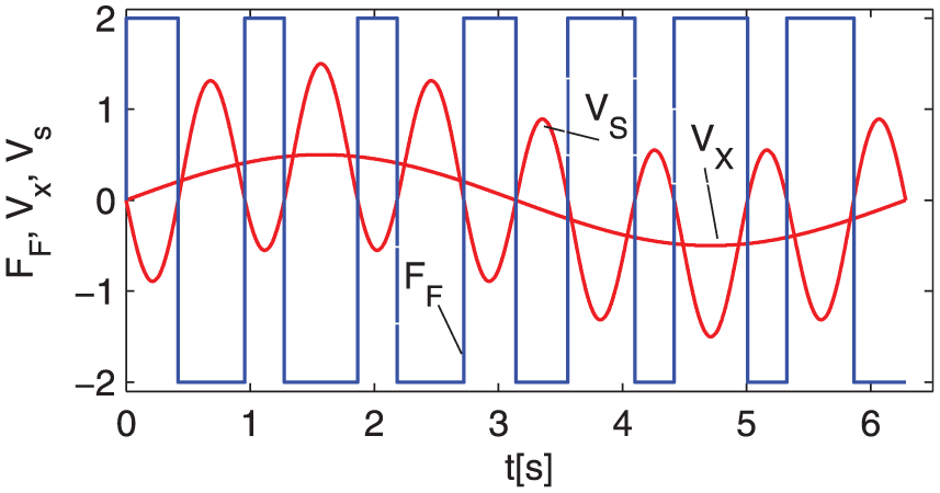When the system is forced to move, the resultant slip velocity between the mass and the plane surface V_s can be described as the difference between the mass velocity V_x and the dither velocity $\overset{\cdot}{d}$ . Assuming friction is governed by a simple Coulomb model, the friction force reaches the value +/–F_C depending on the slip velocity sign, where F_C denotes the Coulomb friction force. Please note that time periods when the friction force reaches positive or negative F_C value are not equal. These frequent changes result in smoothing and reducing the friction force at a macro scale. The plot of a modified friction force is shown in Figure 1.

Figure 1.

Friction modified by dither co-linear with body velocity. V_s: slip velocity; F_F: friction force; V_x: body velocity.

Assume now that the plane surface from the above example moves in a direction perpendicular to the spring axis. What is more, the mass is now between guide plates, which enables motion only co-linear with the spring axis and perpendicular to the motion of the plane surface. When the mass and the surface beneath are in motion, the resultant slip velocity vector consists of two Cartesian components: the mass velocity V_x and the dither velocity $\overset{\cdot}{d}$ . The direction of the friction force vector is opposite the resultant slip velocity. This means that dither perpendicular to the body velocity actually makes the friction two-dimensional (2D). Components of the friction force are proportional to components of the slip velocity, as follows:

\frac{F_{F X}}{F_{C}} = \frac{V_{x}}{V_{s}} .

(1)

This means that the friction force component co-linear with the body velocity F_FX is modulated by both body and dither velocities. Having in mind that the dither velocity is much higher than the mass velocity, one can predict that the resultant slip velocity (and the friction force vector) is almost co-linear with a dither direction. However, in certain time periods, when the dither velocity is achieving values close to zero, the slip velocity changes its direction to co-linear with the body velocity, and the F_FX component of the friction force rises steeply to achieve an Fc value in the time instant when the dither velocity is equal to zero. This means that the F_FX component value changes in a very rapid manner. These changes smooth friction co-linear with the mass velocity at the macro scale.

The time history of modified friction force is shown in Figure 2. The plots in Figures 1 and 2 are not the simulation results. They just show an idea of the mechanism of smoothing dry friction by dither. The brief description given so far can be treated as an introduction to a detailed analysis of the mechanism of smoothing dry friction by dither presented by Piotrowski [5].

Figure 2.

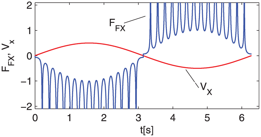
Friction modified by dither perpendicular to the body velocity (F_FX is the friction force component co-linear with body velocity V_x).

3. The new model of two-dimensional dry friction

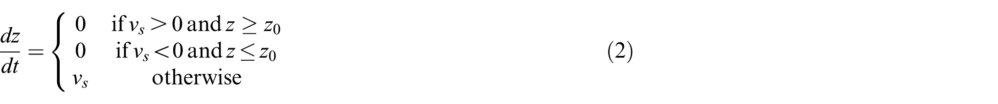
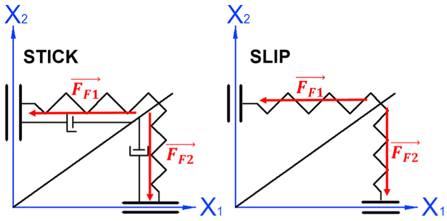
The developed friction model is a 2D interpretation of the RIM, presented by Friedland and Haessig in 1991 [3]. The bristle theory introduced and developed by Friedland and Haessig [3] concerns friction as an effect of contact and deformation of irregularities of contacting surfaces. In the RIM, this effect is approximated by a single bristle. The strain of the bristle (z) is an internal state variable of the model. Strain increases until the limiting value z₀ is reached, which can be interpreted as the stiction range. After reaching this value, strain is kept on a constant level, which represents a slipping phase of the studied motion. An idea of the bristle’s strain and generation of the friction force is presented in Figure 3, where the variable z is governed by the following equation:

\frac{dz}{dt} = {\begin{matrix} 0 & if v_{s} > 0 and z \geq z_{0} \\ 0 & if v_{s} < 0 and z \leq z_{0} \\ v_{s} & otherwise \end{matrix}

(2)

Figure 3.

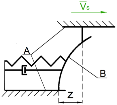
Bristle deformation. A: contacting bodies; B: bristle; Z: the bristle’s strain.

The friction force is divided into static and kinetic friction, whereas the bristle’s strain z plays the role of a switching variable:

F_{F} = {\begin{matrix} σ_{0} (1 + a) z + σ_{1} \frac{dz}{dt} & if | z | < z_{0} \\ σ_{0} z & if | z | \geq z_{0} \end{matrix}

(3)

In equation (3)σ₀ is bristle stiffness, a is stiction gradient and σ₁ represents the damping parameter.

In Xia [6], the 2D model for investigation of stick-slip motion is presented. Components of the friction force are calculated on the basis of the friction direction angle concept, which is defined by both slip velocity and the applied force. On the other hand, the friction model presented by Piotrowski [5] allows for introducing anisotropy into the friction force description. The friction force angle is chosen using the principle of maximum energy dissipation. Both models can be considered as one-dimensional models that are rotated with respect to the vector of slip velocity. However, this approach cannot be applied to convert dynamic friction models into 2D space. It is especially useless as far as interpretation of the internal state variable is based on the bristle theory. Simple rotation of such a model results in a loss of capturing the spring-like behaviour before gross sliding occurs. It could even lead to not detecting the transition between the sticking and slipping phase of the studied motion. The frictional lag phenomenon is also lost. In conclusion, the majority of advantages of these models are lost. This is why a different approach is highly required with respect to transformation of bristle models into a 2D space.

The role of the basic parameter of every bristle model is played by a stiction range. In the case of a planar motion, the stiction range should be described by the following planar set (see also [5]):

Θ_{z} = {Z \in ℝ^{2}, Φ_{z} (Z) \leq 0} .

(4)

In our further investigation Φz(Z) is governed by a circle formula with a radius being equal to the required pre-sliding displacement. In other words, it means that the isotropic stiction range has been assumed.

In order to obtain an appropriate physical character of the bristle model, its 2D interpretation must ensure deforming the bristle in two directions and hold the resultant deformation during the slipping phase of motion. In the planar motion, slip velocity can change its direction without obtaining a value equal to zero or even without changing this value at all. This means that in the slipping phase the deformation of the bristle must be held at the same level, while its components may change. One may say that the bristle “rotates to the direction of a slip”. The consideration carried out so far leads to a division of the bristle deformation into two components, that is, rotation and strain. This division gives motivation to choose polar coordinates as the appropriate ones for description of the bristle deformation:

Z = [\begin{matrix} z_{r} \\ z_{φ} \end{matrix}] .

(5)

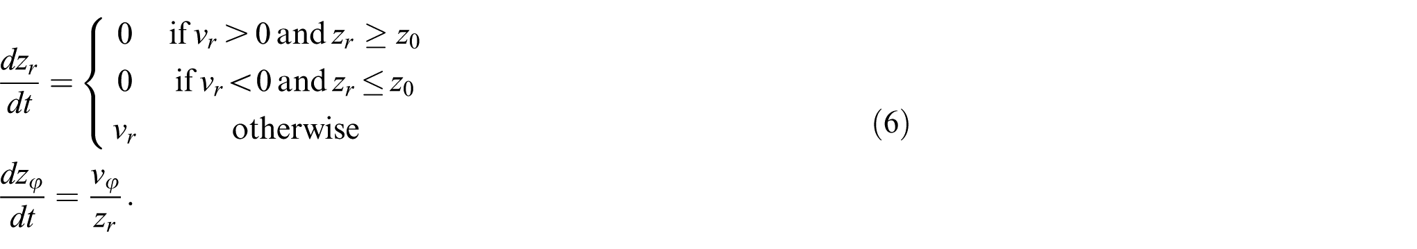
This choice has its consequences in the description of the internal state variable Z. Slip velocity is distributed into two components: rotational v_φ and radial v_r, which is co-linear with the deformed bristle. The mechanism of this division is shown in Figure 4. A rotational component v_φ forces the bristle to rotate into the current slip velocity direction, whereas radial component v_r is responsible for regulation of the bristle’s strain.

Figure 4.

Mechanism of the dividing slip velocity.

The resulting description of dynamics of the variable Z is governed by the following equations:

\begin{matrix} \frac{d z_{r}}{dt} = {\begin{matrix} 0 & if v_{r} > 0 and z_{r} \geq z_{0} \\ 0 & if v_{r} < 0 and z_{r} \leq z_{0} \\ v_{r} & otherwise \end{matrix} \\ \frac{d z_{φ}}{dt} = \frac{v_{φ}}{z_{r}} . \end{matrix}

(6)

The friction force originates from bending of the bristle. The scheme shown in Figure 5 illustrates an idea of generating a 2D vector of the friction force. Although the bristle deformation is described by polar coordinates, the resulting friction force is given in Cartesian coordinates. In order to make our model more application-oriented, the transition into polar coordinates is carried out inside the model. It means that both the input and output of the model are presented in Cartesian coordinates. Like in the RIM, two different components of the sticking and slipping phase are introduced while describing the friction force:

F_{F} = [\begin{matrix} F_{F 1} \\ F_{F 2} \end{matrix}] = {\begin{matrix} [\begin{matrix} σ_{01} (1 + a_{1}) z_{1} + σ_{11} {\dot{x}}_{1} \\ σ_{02} (1 + a_{2}) z_{2} + σ_{12} {\dot{x}}_{2} \end{matrix}] & if z_{r} < z_{0} \\ [\begin{matrix} σ_{01} z_{1} \\ σ_{02} z_{2} \end{matrix}] & if z_{r} \geq z_{0} \end{matrix}

(7)

Figure 5.

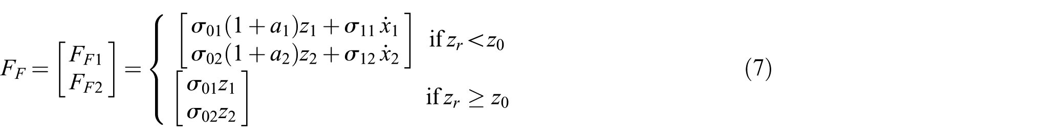
Idea of generating a two-dimensional friction force.

The description of the friction force by equation (7) makes it possible to use hints from Friedland and Haessig [3] regarding a selection of parameters of the model. Even though the stiction range is assumed to be isotropic, an anisotropy of friction can be introduced in the description of each friction force component separately. Actually, three parameters are introduced for both directions, where each of the parameters can be set independently of others.

A few numerical experiments concerning an application of the new friction model exhibiting the introduced damping parameters σ₁₁ and σ₁₂ as velocity dependent have been carried out. Actually, these parameters decrease with velocity increasing, owing to the following formula [1]:

σ_{1} (v_{s}) = σ_{1} \exp [- {(\frac{v_{s}}{a_{v}})}^{2}],

(8)

where the parameter a_v is small (for instance of order 10⁻²).

3.1. Numerical experiments with the new friction model

In order to validate the numerical computation, a simple planar oscillator (Figure 6(a)) has been studied with the following fixed parameters and initial conditions:

friction parameters: σ₀₁ = σ₀₂= 10⁴ [N m⁻¹], σ₁₁ = σ₁₂ = 74.15 [N s m⁻¹], a = 0.1[-], z₀ = 10⁻⁴ [m];

oscillator parameters: m = 1 [kg], k₁ = k₂ = 100 [N m⁻¹];

initial conditions: x₁(t₀) = x₂(t₀) = 0.08 [m], v₁(t₀) = −0.8 [m s⁻¹], v₂(t₀) = 0.8 [ms⁻¹], z_r(t0) = 10⁻⁴ [m], z_φ(t₀) = $135 [\circ]$ .

Figure 6.

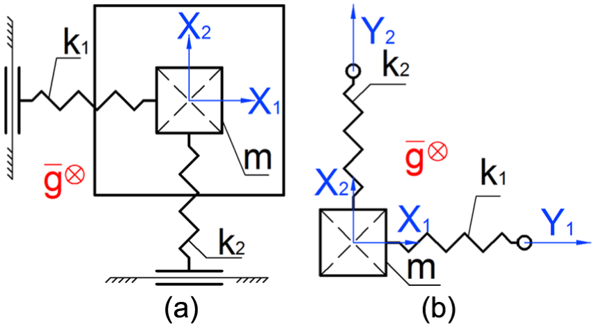
Planar oscillator (a) and a spring-mass system for stick-slip investigation (b).

Displacement of the body in two perpendicular directions is shown in Figure 7. Observe that both x₁ and x₂ displacements are decaying with straight-line envelopes, which is a characteristic feature for motion damped by dry friction. Figure 8(b) shows a polar diagram of radial and rotational components of the internal state variable Z. Actually, this diagram shows a trajectory of the bristle deformation during the simulated motion. As can be seen, components of 2D friction force (Figure 8(a)) are proportional to the bristle’s deformation except the place where sticking phase begins, which has to be expected.

Figure 7.

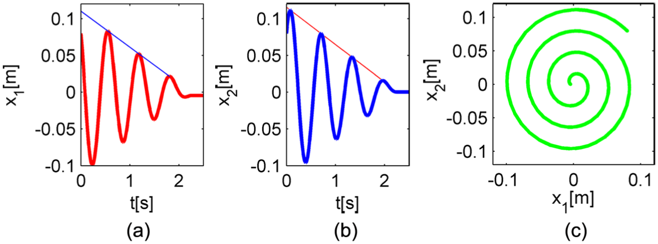
Simulation results: displacements (a) x₁(t) and (b) x₂(t) versus time and (c) a trajectory.

Figure 8.

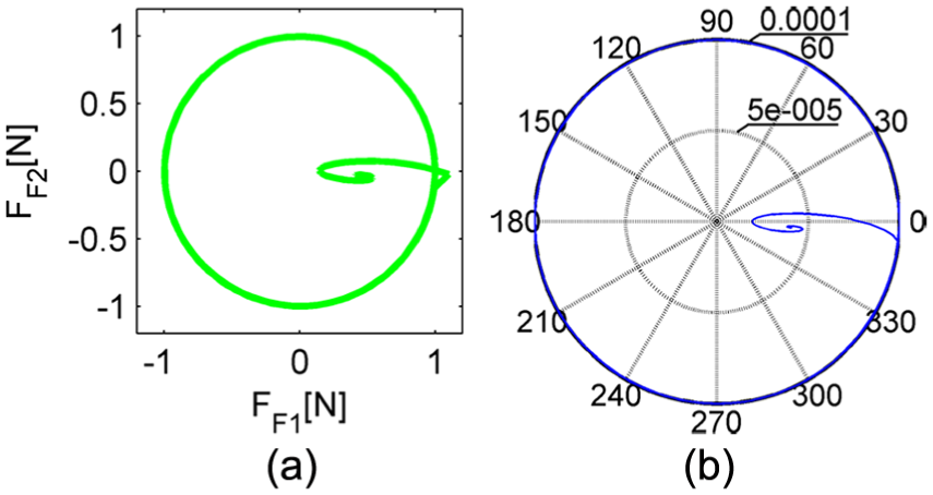
Simulation results: (a) the two-dimensional friction force; (b) the bristle trajectory.

Next, an experiment concerning 2D stick-slip behaviour has been conducted regarding the system shown in Figure 6(b) and for the following fixed parameters: x₁(t₀) = x₂(t₀) = 0 [m], v₁(t₀) = v₂(t₀) = 0 [m s⁻¹], z_r(t₀) = 0 [m], z_φ(t₀) = $0 [\circ]$ , v_y₁ = 0.01 [ms⁻¹], v_y₂ = 0.005 [m s⁻¹], v_y₁ = v_y₂ = const. Friction and system parameters are the same as in the previous simulation.

Figures 9 and 10 present the results of the simulation, which capture 2D stick-slip behaviour. In the reported time histories (Figure 9) characteristic sticking and slipping phases of the motion are visible. Slopes of these plots correspond to the fixed velocities v_y₁ and v_y₂. Switching between two regimes of the studied motion occurs simultaneously in both directions, which is physically expected. This behaviour is also observable in diagrams of the friction force time histories (Figure 10). Observe that a proportion of the values of the friction force components is the same as the proportion of the velocities v_y₁ and v_y₂, which has to be expected. The carried out numerical experiment proves the correctness of capturing 2D stick-slip behaviour.

Figure 9.

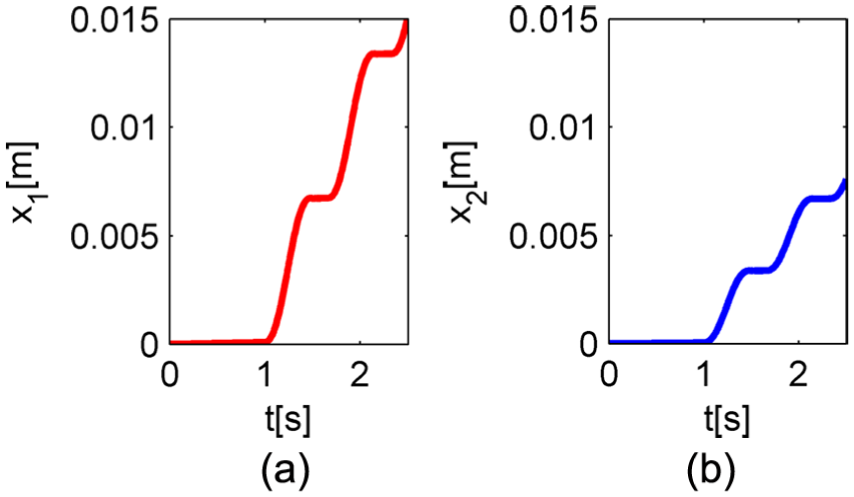
Time histories of the stick-slip behaviour: (a) x₁(t); (b) x₂(t).

Figure 10.

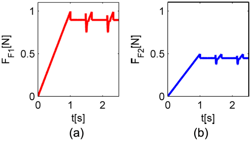
Time histories of the friction force: (a) F_F₁(t); (b) F_F₂(t).

3.1.1. The influence of initial conditions

In order to validate the implemented model of a planar oscillator and the new friction model, a special type of motion should be studied. A proper choice of the initial conditions should give predictable results of the simulation. For the planar oscillator without friction, such a predictable result could be a circular trajectory. Obtaining this trajectory is possible only when certain circumstances are satisfied by oscillator parameters as well as by the introduced initial conditions [5]. Firstly, the spring constants for both degrees of freedom must have the same value: k₁= k₂= k. Secondly, the direction of initial velocity must be perpendicular to the vector of initial displacement. Furthermore, a value of initial velocity must be calculated in a way that results in a balance between the centrifugal force and the reaction coming from the springs. In order to achieve an unambiguous solution from the introduced assumptions, special circumstances must be added. It has been assumed that initial displacement should be in the first quadrant of the coordinate system and the motion should occur in a counter-clockwise direction. These assumptions yielded the following formulas required for the initial conditions:

\begin{matrix} {\overset{\cdot}{x}}_{1} (t_{0}) = \sqrt{\frac{{kx}_{2}^{2} (t_{0})}{m}}, {\overset{\cdot}{x}}_{2} (t_{0}) = \sqrt{\frac{k r^{2}}{m} - {\overset{\cdot}{x}}_{1}^{2} (t_{0})} \\ r = \sqrt{x_{1}^{2} (t_{0}) + x_{2}^{2} (t_{0})} . \end{matrix}

(9)

Applying the initial conditions (9) allowed one to achieve the expected circular trajectory. After adding friction to the oscillator’s model, the trajectory should change to a spiral one, which indeed happened.

4. Validation of the introduced model

The carried out validation of the introduced model consists of three steps. Firstly, smoothing dry friction by dither is verified in Section 4.1 regarding time histories and friction force in two perpendicular directions. Secondly, the introduced model has been validated experimentally in Section 4.3 regarding planar motion with and without presence of a dither.

4.1. Numerical test

In order to check if the proposed model captures correctly the mechanism of smoothing dry friction by dither, the latter has been introduced in the x₂ direction in the form $d_{2} = 0.005 \sin (500 t)$ .

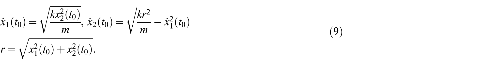
Figure 11 presents x₁ and x₂ displacements versus time, and one may observe that the envelopes indicate the occurrence of viscous damping. In addition, the directional effect of the introduced dither has been captured. In other words, motion co-linear with dither is lightly damped in comparison to the perpendicular one.

Figure 11.

Displacement time histories: (a) x₁(t); (b) x₂(t).

Figure 12 presents friction force components in the time domain. Both co-linear and perpendicular components have a similar form, which validates the theoretical prediction.

Figure 12.

Friction force time histories: (a) F_F₁(t); (b) F_F₂(t).

4.2. Experimental rig

The laboratory rig has the form of a spherical pendulum. The pendulum is suspended by a special joint that enables a movement in two degrees of freedom. Actually, this joint is known from the automotive industry as a homokinetic joint. The set is mounted in a way that prevents rotation of the rod around its axis. Inside the massive body that is fixed to the rod, there is a specimen of the tested material. In motion, the specimen slides over the spherical surface and the contact friction is considered as a 2D one. The specimen is driven by a vibration generator that plays the role of dither.

In the plane containing the point of pendulum suspension, there is a rim whose displacement is measured by two sensors. The results of these measurements can be easily recalculated into two components of displacement of the body or the specimen (see Figure 13).

Figure 13.

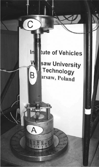
Laboratory rig. A: massive body; B: vibration generator; C: joint and rim [5].

The modelling of the experimental rig and the introduced simplifications are presented in the Appendix.

4.3. Verification of the new 2D friction model

Two runs of the pendulum have been recorded in the experimental part. In the first case, no dither occurred and the results of the run were used to identify friction parameters. The trajectory recorded in the second run (with dither) was used to verify the new friction model regarding dry friction modification by dither. Initial conditions of the recorded motion, that is, displacement and velocity, have been calculated numerically from the obtained results, since the pendulum has been propelled manually.

Figure 14 shows components of the recorded displacement for the experimental run without dither. The following straight lines describing the recorded decaying motion have been found:

x_{1} (t) = - 0.00822 t + 0.032, x_{2} (t) = - 0.00803 t + 0.032 .

(10)

Figure 14.

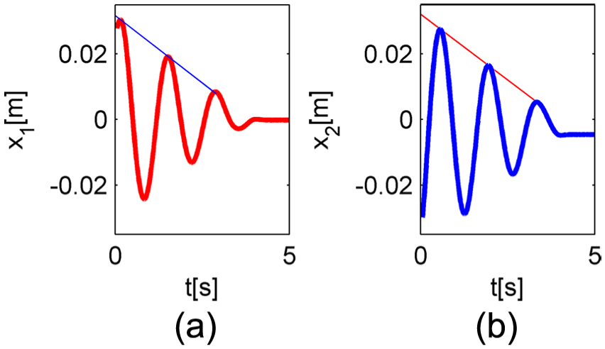
Time histories without dither, obtained experimentally: (a) x₁(t); (b) x₂(t).

Identification of friction parameters has been carried out by achieving the same slope of these lines. Damping parameters σ₁₁ and σ₁₂ have been calculated in a way similar to that proposed by Friedland and Haessig [3], resulting in a damping coefficient of 0.707. Both trajectories, that is, experimental and numerical ones, are reported in Figure 15. The obtained envelopes have been described by the following straight-line equations:

x_{1} (t) = - 0.00822 t + 0.031, x_{2} (t) = - 0.00803 t + 0.039 .

(11)

The following friction parameters have been taken: σ₀₁ = 7293.7 [N m⁻¹], σ₀₂ = 5572.08 [N m⁻¹], σ₁₁ = 209.2 [N sm⁻¹], σ₁₂ = 182.8 [N sm¹], a₁= a₂= 0.2 [-], z₀= 10⁻⁴ [m].

Figure 15.

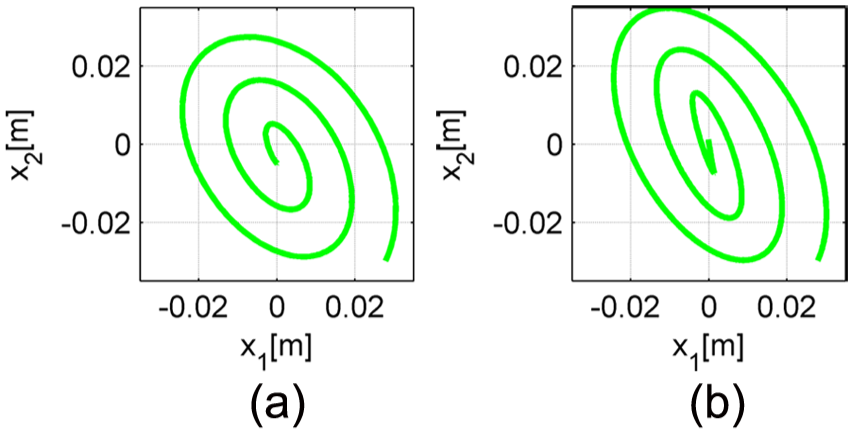
Plots x₁(x₂) without dither: (a) experiment; (b) simulation.

Since the pendulum has already moved at the time instant when measurement started, the initial state of the model has been set as follows. The strain of the bristle has been set to a value equal to the radius of the stiction range, whereas the rotation z_φ has been set to be co-linear with the direction of slip velocity.

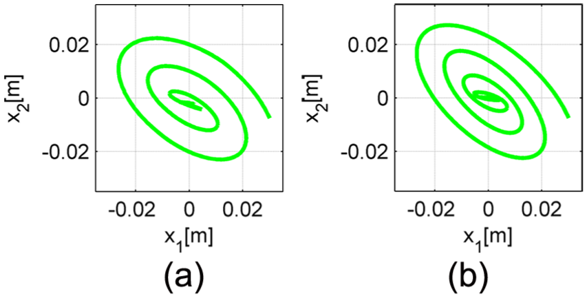
In the next step of validation, we compare the experimental runs with dither and the corresponding numerical results (see Figure 16). In the mathematical model of the laboratory rig, dither has been introduced in the x₁ direction and modelled by the following harmonic function: $\overset{\cdot}{d} = A ω \cos (ω t)$ , A = 0.0004 [m], ω = 219.9 [s⁻¹].

Figure 16.

Plots x₁(x₂) with dither: (a) experiment; (b) simulation.

The parameters of dither have been set as in Piotrowski [5]. The trajectory recorded during the experimental run and the trajectory obtained from numerical simulation are shown in Figure 16. The initial state of the friction model has been set according to the same standards as previously. The trajectories obtained from modelling are similar to those recorded during the experimental runs, which validates our introduced 2D friction model.

Observe that the envelopes of the trajectories presented in Figure 17 are straight lines at the beginning, and then they transit into exponential ones. This statement is indeed true. It is impossible to fit exponential envelopes to displacements x₁ and x₂ shown in Figure 17. In the early phase of the recorded run, the velocity of the body was too high in comparison to dither velocity and the effect of modification did not occur. This fact is also visible in a plot of bristle strain z_r versus time, obtained from simulation. The variable z_r is found inside the stiction range after about 2 s. This means that the earlier modification effect could have not occurred.

Figure 17.

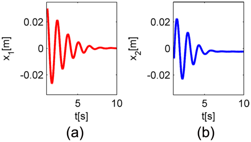
Time histories with dither, obtained experimentally: (a) x₁(t); (b) x₂(t).

5. Conclusions

A new model of 2D friction has been proposed and validated both numerically and experimentally. The proposed model is a 2D interpretation of the RIM presented by Friedland and Haessig [3] as a more computationally efficient version of the bristle model (presented in the same paper). The one-dimensional model was converted into a 2D space with the use of the original 2D bristle concept. The model developed by us allows for introducing anisotropy of friction in the bristle parameters. The model has been tested numerically regarding capturing the 2D stick-slip effect and mechanism of smoothing friction by dither. Furthermore, the experimental verification has been carried out using a special laboratory rig. The carried-out laboratory experiments dealt with 2D friction both modified and unmodified by dither. The results obtained from the experiment and numerical simulations have shown good similarity, which validates our 2D friction model.

In comparison to the model presented by Piotrowski [5], our model is more general regarding the description of the friction phenomenon. It accounts for a static friction effect, what is critical with respect to the detection of stick-slip motion. The model from Piotrowski [5] captures spring-like behaviour before gross sliding occurs and pre-sliding displacement effect. However, in this model the stiction range is a resultant value from a spring constant and a break-away force, whereas in our model this parameter is set independently. Due to the 2D bristle concept our model transfers friction memory into 2D space. This effect can be highly important regarding investigation of a dither with more complex form then the sinusoidal one. In contrast to the model from Piotrowski [5], ours has a damping term in its description. However, it has to be mentioned that Piotrowski in [7] employed the upgraded model with introduced damping, which essentially improved the modelling of the dither smoothing effect.

Footnotes

Appendix: Mathematical model of the laboratory rig

The following simplification has been introduced while modelling the laboratory rig. Friction in the joint has been assumed to be relatively low due to the joint construction. The rod is treated as a mass-less and rigid element, since it is more than 10 times lighter than the body.

Typically, in modelling a spherical pendulum, the coordinates used to describe the position of the mass are spherical. However, in our case the use of this set of coordinates would be impractical. Figure 18(a) shows the surrogate set-up of the joint and the applied corresponding coordinates.

The mathematical model of the laboratory rig has been developed regarding Lagrangian mechanics. Calculations have been carried out as follows. Coordinates of the point mass follow:

(12)

x_{1} = l \sin φ, x_{2} = l \sin θ \cos φ, x_{3} = l (1 - \cos θ \cos φ) .

Lagrangian is defined as

(13)

L = T - V,

and T is the kinetic energy and V stands for the potential energy of the system:

(14)

T = \frac{1}{2} m v^{2}, V = mgz, v = \sqrt{l^{2} (\overset{\cdot}{φ} + \overset{\cdot}{θ} \cos^{2} φ)} .

Putting equations (14) into (13) yields

(15)

L = - \frac{1}{2} ml (l {\overset{\cdot}{φ}}^{2} + l {\overset{\cdot}{θ}}^{2} g \cos^{2} φ + 2 g \cos θ \cos φ) .

Equations of motion have been calculated from Lagrange’s equations of the second kind, of the forms

(16)

\begin{matrix} \frac{d}{dt} (\frac{\partial L}{\partial \overset{\cdot}{θ}}) - \frac{\partial L}{\partial θ} = τ_{1}, \\ \frac{d}{dt} (\frac{\partial L}{\partial \overset{\cdot}{φ}}) - \frac{\partial L}{\partial φ} = τ_{2} . \end{matrix}

Moments of the external forces in equation (16) are

(17)

τ_{1} = F_{F 2} l_{F} \cos φ, τ_{2} = F_{F 1} l_{F}

where l_F is the total length of the considered pendulum. The final form of the equations of motion is as follows:

(18)

\begin{matrix} \overset{\cdot\cdot}{θ} = \frac{2 m l^{2} \overset{\cdot}{θ} \overset{\cdot}{φ} \cos φ \sin φ - mlg \sin θ \cos φ + τ_{1}}{m l^{2} \cos^{2} φ}, \\ \overset{\cdot\cdot}{φ} = \frac{τ_{2} - m l^{2} {\overset{\cdot}{θ}}^{2} \cos φ \sin φ - mlg \cos θ \sin φ}{m l^{2}} . \end{matrix}

As the case concerned the planar oscillator model, the mathematical model of the laboratory rig had to be validated. Again, proper initial conditions were needed in order to give predictable simulation results. As a predictable result a circular trajectory has been chosen and to find proper initial conditions a kinetostatic analysis has been performed. The first circumstance that must be fulfilled is a balance between the forces shown in the Figure 19. Secondly, the initial velocity has to be perpendicular to the initial displacement vector. The carried-out analysis has resulted in the following formula for the initial conditions:

(19)

\begin{matrix} θ (t_{0}) = θ_{0}, φ (t_{0}) = 0, \overset{\cdot}{θ} (t_{0}) = 0, \\ \overset{\cdot}{φ} (t_{0}) = \frac{\sqrt{gl \cos θ_{0} si n^{2} θ_{0} (\sin^{2} θ_{0} - si n^{4} θ_{0})} \sin θ_{0}}{l (\sin^{4} θ_{0} - si n^{2} θ_{0})} . \end{matrix}

Regarding the initial conditions (19), the resultant trajectory should have the form of a circle with the radius equal to $l \sin θ (t_{0})$ . Validation of the aforementioned has been carried out for the following fixed parameters: $θ (t_{0}) = 15 [\circ]$ , $φ (t_{0}) = 0 [\circ]$ , $\overset{\cdot}{θ} (t_{0}) = 0 [s^{- 1}]$ , $\overset{\cdot}{φ} (t_{0}) = - 1, 2296 [s^{- 1}]$ . The expected trajectory radius is equal to 0.1165 [m]. This value has been obtained, which has validated the correctness of our laboratory rig model.

After verification of the mathematical model, friction between the specimen and spherical surface has been added. In this case, physical interpretation is such that the bristle is mounted at the end of the specimen and a loose end of the bristle is in contact with a spherical surface underneath. The abovementioned has consequences in the sign of slip velocity components given in the input to the model.

Funding

The work was supported by the Polish National Science Centre, MAESTRO 2 (grant number 2012/04/A/ST8/00738).

References

Canudas de Wit

Gafvert

Lischinsky

. Friction models and friction compensation. Eur J Contr 1998; 4: 176–195.

Dahl

PR.

A solid friction model. Report. The Aerospace Corporation, California, 1968.

Friedland

Jr Haessig

DA.

On the modeling and simulation of friction. J Dynam Syst Meas Contr 1991; 113: 354–362.

De Wit

Olsson

Astrom

. A new model for control of systems with friction. IEEE Trans Autom Contr 1995; 40(3): 419–425.

Piotrowski

Smoothing dry friction damping by dither generated in rolling contact of wheel and rail and its influence on ride dynamics of freight wagons. Int J Vehicle Mech Mobil 2010; 48(6): 675–703.

Xia

Modelling of a two-dimensional coulomb friction oscillator. J Sound Vibr 2002; 265(2003): 1063–1074.

Piotrowski

A substitute model of two-dimensional dry friction exposed to dither generated by rolling contact of wheel and rail. Int J Vehicle Mech Mobil 2012; 50(10): 1495–1514.