Does convexity of yield surfaces in plasticity have a physical significance?

Abstract

Convexity of a function or set is an often needed and important mathematical property. In the case of yield functions $ϕ (T)$ (or elastic ranges) in terms of stresses, almost all empirical and mechanism-based yield functions have this property. However, requiring positive plastic dissipation does not necessarily exclude non-convex yield functions, which is confirmed by the fact that non-convex yield functions are observed experimentally, although this rarely happens. We therefore ask whether this nice mathematical property reflects a physical material property. This is investigated in an elastic–plastic, small strain, 2D setting. It appears that, at least in this setting, no specific material property can be attributed to the convexity of the yield function.

Keywords

Plasticity yield function convexity

1. Introduction

Some kind of convexity is usually necessary for minimization problems to have a unique solution, like quasiconvexity of the strain energy in nonlinear elasticity. Based on Drucker’s postulate [1], the convexity of yield function $ϕ (T) \leq 0$ in the stress space is associated with material stability. This somehow suggests itself, since the yield function has a potential character in associative plasticity. In that case, the plastic strain rate ${\dot{E}}_{p}$ is parallel to the gradient of $ϕ (T)$

\begin{matrix} {\dot{E}}_{p} = λ ϕ^{'} (T) . \end{matrix}

(1)

The plastic multiplier λ is determined such that the stress state $T$ is on the yield function during plastic flow, that is, such that $ϕ (T) = 0$ and $\dot{ϕ} (T) = 0$ during plastic flow.

There are some indications that convexity of the yield function in stress space is too strict. Krawietz [2] attests Drucker’s method to be useful, but states that Drucker’s conclusions are flawed. Drucker requires positivity of the path integral

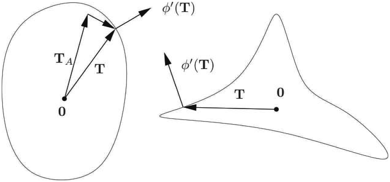
\begin{matrix} 0 \leq \oint (T - T_{A}) \cdot \cdot d E, \end{matrix}

(2)

where $T$ is the current stress state, while the role of the constant stresses $T_{A}$ is unclear. Drucker refers to stresses exerted by an external agency. They can take any value in the elastic range. Presuming an associated flow rule, this inequality holds only in the case of convex yield functions. Only, if we take $T_{A} = O$ , this path integral becomes the energy dissipated in such a process, that is, it can be interpreted physically. Requiring a positive dissipation in any circular stress-process that involves plastic flow, we arrive at star convexity with respect to $T = O$ of the yield function (see [3, p. 280] or [4, p. 523]); refer to Figure 1 for a sketch. Drucker’s method basically leads to the requirement that the elastic range is star-convex from any point within the elastic range, which results in the convexity of the elastic range. A more thorough discussion of material stability including large strains may be found in [5, 6], where [5] gives a concise summary of Druckers results. In the small strain setting, a review including a historical note is available in [7].

Figure 1.

Convexity vs star convexity of the yield surface in the stress space. Star convexity is sufficient to guarantee positivity of the scalar product T ⋅⋅ $ϕ^{'}$ (T).

These considerations are largely uninteresting for many materials, the flow behaviour of which is well modelled by convex yield criteria. In fact, apparently all empirical or physical yield criteria are convex, like the ones of Mises, Tresca, Hill, Mohr–Coloumb and Schmidt. Nevertheless, some materials exhibit non-convex yield functions. We have encountered such yield surfaces in the homogenization of a honeycomb structure, but they have been observed before for solid metals as well; see [8, 9].

Thus, if we allow for star-convex yield functions together with an associative flow rule, it remains to discuss which qualitative material properties are reflected by the mathematical property of the convexity of $ϕ (T)$ , if any. For example, Ortiz and Repetto [10, p. 457] state that convexity of the yield function is sufficient to suppress the evolution of fine micro-structures. But, conversely, does non-convexity imply such material behaviour? This question is examined in this article in a phenomenological, descriptive manner.

The starting point is the two-dimensional elastic–plastic problem with an isotropic, Mises-like yield function in the small strain setting. This allows us to examine the yield function in the three-dimensional space where $T_{11}$ , $T_{22}$ and $T_{12}$ are perpendicular axes, such that (non-)convexity is immediately apparent. The Mises-like yield function is a cylinder with an elliptical base plane parallel to the hydrostatic axis $T_{11} e_{1} + T_{22} e_{2}$ . We then describe this Mises cylinder in polar coordinates, on which we impose bumps to generate pressure-insensitive, anisotropic yield functions, the convexity of which is controlled by the amplitude of the bumps. We then carry out finite element simulations, which are checked for qualitative material behaviour changes as the yield function becomes non-convex.

2. Example for a non-convex elastic range

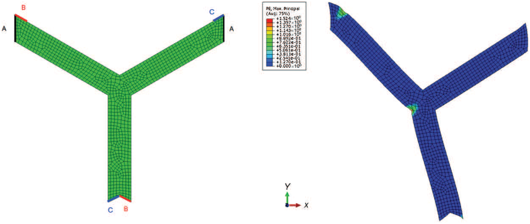
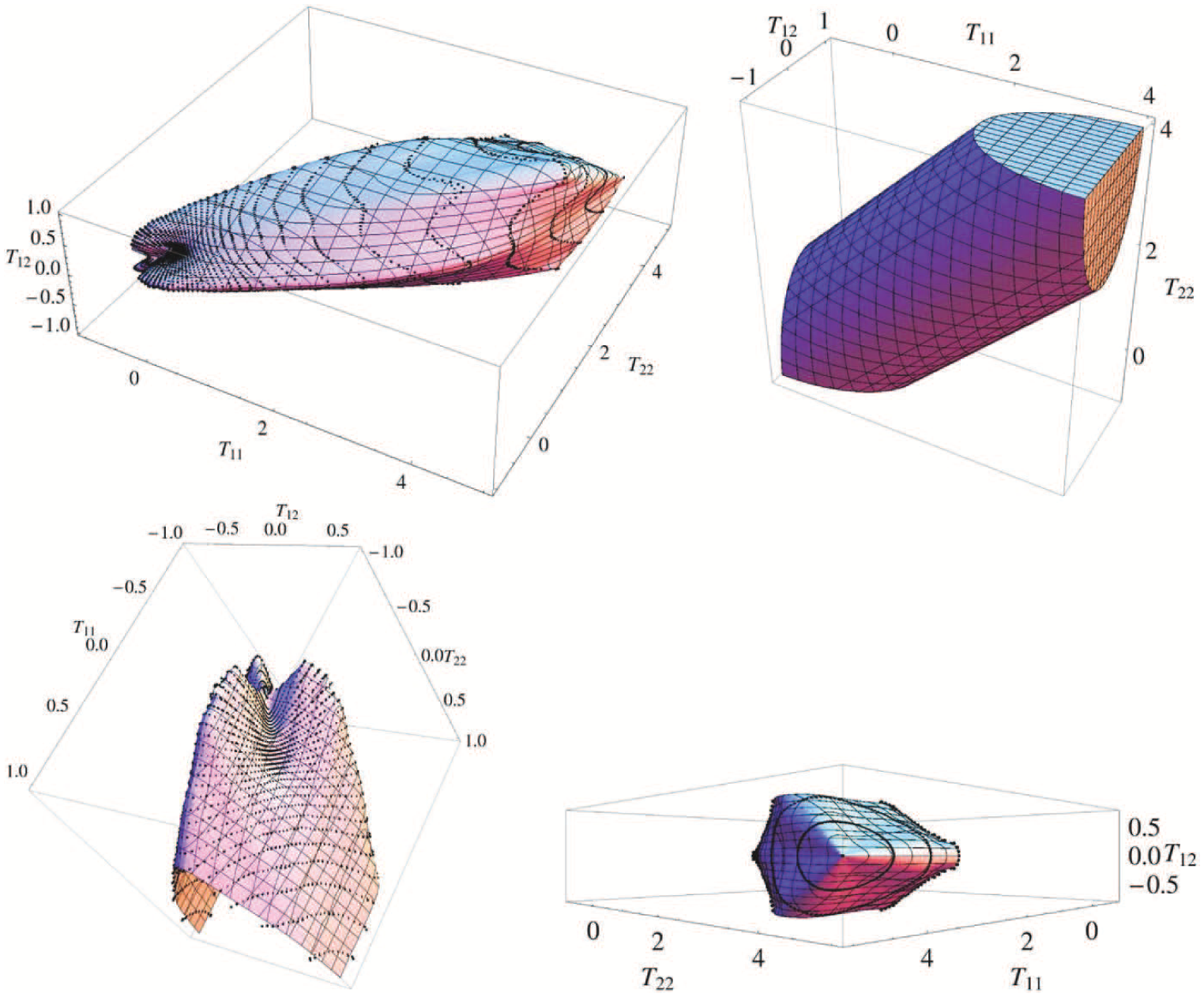
We now give a simple example of a non-convex yield function. It emerges from the study of the elastic–plastic behaviour of regular honeycomb structures. After a parametrization of the plane stress state with the stress tensor magnitude, the eigenstress direction with respect to the honeycomb structure and a loading type parameter $χ = \arctan (σ_{2} / σ_{1})$ in terms of the stress eigenvalues, we performed numerical simulations on a representative volume element (RVE; see e.g. [11 –14]): see Figure 2. The RVE consists of a Y-shaped unit cell with periodic boundary conditions, employing common isotropic Mises plasticity on the micro-scale. Stress-driven tests with monotonically increasing stress magnitudes and fixed eigendirections and eigenvalue ratios were performed. The resulting stress–strain curves display a smooth transition from the elastic to the plastic range, since yielding takes place localized at the strut’s connections, which act like plastic hinges. Following the approach of [15], we extracted the effective yield point assuming that plasticity occurs when 10% of the total stress power is dissipated in plastic deformations. The resulting yield surface is plotted in Figure 3. We can clearly see the non-convexity of the yield surface, which is elongated along the hydrostatic axis. One can see that the material reacts more weakly to hydrostatic compression than to hydrostatic tension. Also, one can recognize the three-fold material symmetry in the yield surface.

Figure 2.

Y-shaped unit cell of the hexagonal structure. The boundary sections A, B and C are coupled by the usual periodic displacement and anti-periodic traction boundary conditions. The colormap indicates the plastic strain amplitude (PE).

Figure 3.

The yield surface of the honeycomb structure (upper left) that is elongated along the hydrostatic axis and the simple plane Mises yield criterion (upper right) with $σ_{crit} = 1$ MPa in the stress space $T_{11}, T_{22}, T_{12}$ . The black dots represent the yield points resulting from RVE finite element simulations, on which the interpolated yield surface is constructed. The lower figures show details of the yield surface of the honeycomb structure, namely the bumps near the compressive end of the yield surface (lower left), and a view parallel to the hydrostatic axis towards the origin (lower right), in which the spatial six-fold symmetry is manifested as a three-fold symmetry in the stress space.

3. 2D plasticity

3.1. The model

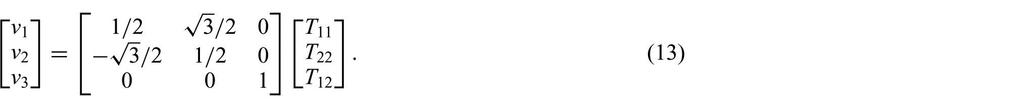
We use the two-dimensional orthonormal basis $e_{i}$ to set up our two-dimensional model in tensor notation, and the three-dimensional orthogonal basis $r_{i}$ to graphically represent plane stress states. Thus, we can write the Cauchy stresses as

\begin{matrix} T & = T_{11} e_{1} \otimes e_{1} + T_{22} e_{2} \otimes e_{2} + T_{12} (e_{1} \otimes e_{2} + e_{2} \otimes e_{1}) \end{matrix}

(3)

\begin{matrix} = T_{11} r_{1} + T_{22} r_{2} + T_{12} r_{3} . \end{matrix}

(4)

It should be clear from the context which basis is being used. The corresponding strain tensor is

\begin{matrix} E & = u_{1, 1} e_{1} \otimes e_{1} + u_{2, 2} e_{2} \otimes e_{2} + \frac{u_{1, 2} + u_{2, 1}}{2} (e_{1} \otimes e_{2} + e_{2} \otimes e_{1}) \end{matrix}

(5)

with the plane displacement field $u = u_{1} (x_{1}, x_{2}) e_{1} + u_{2} (x_{1}, x_{2}) e_{2}$ and the partial derivatives with respect to $x_{1}$ and $x_{2}$ denoted by a comma. We employ the additive strain decomposition of the overall strain $E$ into the elastic strains $E_{e}$ and the plastic strains $E_{p}$ ,

\begin{matrix} E = E_{e} + E_{p}, \end{matrix}

(6)

as usual in the small displacement setting. The isotropic elastic law is expressed as a matrix–vector product involving the components of $T$ and $E_{e}$ ,

\begin{matrix} [\begin{matrix} T_{11} \\ T_{22} \\ T_{12} \end{matrix}] & = \frac{E}{1 - ν^{2}} [\begin{matrix} 1 & ν & 0 \\ ν & 1 & 0 \\ 0 & 0 & 1 - ν \end{matrix}] \cdot [\begin{matrix} E_{e 11} \\ E_{e 22} \\ E_{e 12} \end{matrix}], \end{matrix}

(7)

with Young’s modulus E and Poisson’s ratio ν as the elasticity constants. We consider a Mises-like yield function

\begin{matrix} ϕ (T) = \sqrt{2} ∥ T^{'} ∥ - σ_{crit}^{tension} \leq 0 . \end{matrix}

(8)

Note that this is not simply the usual Mises yield function from the three-dimensional case with zero out-of-plane stress components, but a two-dimensional version of it. The stress deviator $T^{'}$ is

\begin{matrix} T^{'} = T - \frac{T_{11} + T_{22}}{2} I . \end{matrix}

(9)

The factor $\sqrt{2}$ serves to normalize the critical equivalent stress $σ_{crit}^{tension}$ such that it can be measured directly in a tension test (in the three-dimensional case the factor is $\sqrt{3 / 2}$ ). We summarize $σ_{crit} = σ_{crit}^{tension} / \sqrt{2}$ :

\begin{matrix} 0 & \geq ∥ T^{'} ∥ - σ_{crit} \end{matrix}

(10)

\begin{matrix} 0 & \geq {(T_{11} - (T_{11} + T_{22}) / 2)}^{2} + {(T_{22} - (T_{11} + T_{22}) / 2)}^{2} + 2 T_{12}^{2} - σ_{crit}^{2} . \end{matrix}

(11)

The region defined by the latter inequality in the three-dimensional space $T_{11}, T_{22}, T_{12}$ is the elastic range. In the space of $r_{i}$ , it appears as a cylinder parallel to the hydrostatic axis $T_{11} r_{1} + T_{22} r_{2}$ with an elliptical base plane, see Figure 3. If we normalize the basis $r_{i}$ the cylinder’s base plane becomes a circle. The ratio of the base ellipse’s half-axes is $\sqrt{2}$ , where the shorter one is parallel to $T_{12} r_{3}$ ; see Figure 3. For plastic flow we use the commonly employed associative flow rule (equation (1)), with the consistency parameter λ such that the stress is on the yield function during plastic flow.

3.2. The model extension

We will now describe the base ellipse in polar coordinates to equip it later with bumps. By this procedure, we preserve the pressure-insensitivity of the yield functions, which become anisotropic.

Let $T = T_{11} r_{1} + T_{22} r_{2} + T_{12} r_{3}$ . Firstly, we rotate the Mises cylinder by − π/4 around the $r_{3}$ -axis, such that the hydrostatic axis is parallel to $r_{1}$ . Then we get

\begin{matrix} v & = Q \cdot T, \end{matrix}

(12)

\begin{matrix} [\begin{matrix} v_{1} \\ v_{2} \\ v_{3} \end{matrix}] & = [\begin{matrix} 1 / 2 & \sqrt{3} / 2 & 0 \\ - \sqrt{3} / 2 & 1 / 2 & 0 \\ 0 & 0 & 1 \end{matrix}] [\begin{matrix} T_{11} \\ T_{22} \\ T_{12} \end{matrix}] . \end{matrix}

(13)

In terms of $v$ we can write the yield function as

\begin{matrix} ϕ (T) & = \sqrt{v_{2}^{2} + 2 v_{3}^{2}} - σ_{crit} . \end{matrix}

(14)

Putting bumps on this ellipse is achieved by making $σ_{crit}$ a function of the angle in the $r_{1}$ -plane,

\begin{matrix} ϕ (T) = \sqrt{v_{2}^{2} + 2 v_{3}^{2}} - σ_{crit} (1 + a \cos (n \arctan (v_{2} / v_{3}))), \end{matrix}

(15)

with a the relative amplitude and n the number of bumps that we put on the yield surface. Setting $ϕ (T) = 0$ and using the substitutions $v_{2} = r \sin (θ)$ and $v_{3} = r \cos (θ)$ we get the polar form

\begin{matrix} r (θ) = σ_{crit} \frac{1 + a \cos (n θ))}{\sqrt{2 \cos {(θ)}^{2} + \sin {(θ)}^{2}}} . \end{matrix}

(16)

Convexity implies that a linear interpolation between any two points in the convex domain is inside the domain. In terms of stresses, the yield function is convex if

\begin{matrix} ϕ (α T_{1}) + ϕ ((1 - α) T_{2}) \leq 0 \leftrightarrow ϕ (T_{1}) \leq 0, ϕ (T_{2}) \leq 0, 0 \leq α \leq 1 . \end{matrix}

(17)

Since a convex domain must be always simply connected, the latter can be replaced by requiring that the domain boundary has a positive curvature, i.e. all eigenvalues of the surface curvature tensor must be positive everywhere on the boundary. Thus, instead of the 3D stress space we consider its 2D boundary, of which the curvature parallel to the hydrostatic axis is zero. The one remaining convexity condition is the positivity of the curvature of the polar base curve $r (θ)$ ,

\begin{matrix} r {(θ)}^{2} + 2 r^{'} {(θ)}^{2} - r (θ) r^{″} (θ) \geq 0 . \end{matrix}

(18)

we can give bounds for a in dependence on n such that the yield function remains convex. Here, we take n=3, which results in - 1/19 ≤ a ≤ 1/19 for the yield function to be convex in the stress space. Convexity is lost at the angle θ = π.

3.3. Implementation

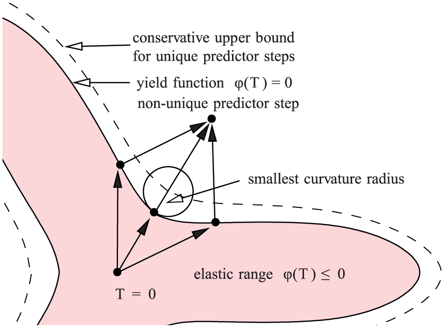
The model is implemented as a subroutine in Abaqus. The user material subroutine and the input file that were used for the Abaqus simulations can be found at http://ifm-hp15.mb.unimagdeburg.de/gluege/SupMat_MMS_17_0091/. The numerical time integration of $E_{p}$ is done with the implicit Euler scheme, which is solved by Newton’s algorithm [16, 17]. Details on the numerics of plane stress plasticity can be found in [18]. The most obvious consequence of a non-convex yield function is that the usual predictor–corrector algorithm becomes ambiguous, that is, the solution to a plastic corrector step may not be unique, and requires more advanced solution techniques [19]. For smooth yield functions, this problem can be avoided by taking only very small steps. For star-shaped yield functions, the smallest curvature radius encountered on the yield surface provides a conservative upper bound for the admissible step size of the predictor step (Figure 4).

Figure 4.

Sketch of the non-convex yield function with a three fold symmetry. A large predictor step gives rise to a non-unique update of ${\dot{E}}_{p}$ , which follows (one of the) the yield surface normals. A conservative upper bound for the predictor step is given by the smallest radius of curvature that is found on the yield function. Thus, it is always possible to follow a unique strain evolution when the step size is sufficiently small.

4. Simulations

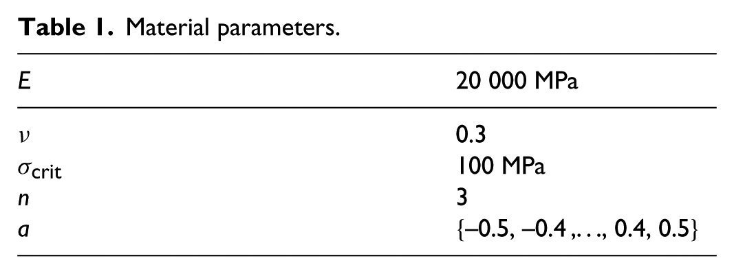
To examine the effect of our modification, we consider a reference simulation and how it changes when smaller or larger bumps are put on the yield surface. The boundary value problem consists of a simple shear deformation of a square with edge length l, where two opposing faces are displaced rigidly by l/10 parallel to each other, while the remaining two faces are free of traction. The material parameters are given in Table 1.

Table 1.

Material parameters.

E	20 000 MPa
ν	0.3
$σ_{crit}$	100 MPa
n	3
a	{ –0.5, –0.4,…, 0.4, 0.5}

The result is somewhat characteristic, symmetrically displaying two curved zones of localized plastic deformation (Figure 5). Parts of the strain localization zone tend to zero thickness, and thus there is a spurious mesh dependence, which may be overcome by a sufficiently high hardening. However, to separate the causes and effects as cleanly as possible, we prefer to leave out hardening, and resume with the most simple possible material law.

Figure 5.

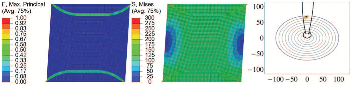
Isotropic, convex reference simulation. Left: Largest absolute strain eigenvalue from 0 (blue) to 1 (red). Center: Equivalent von Mises stress from 0 (blue) to 300 MPa (red). Right: Elastic range projected perpendicular to the hydrostatic axis, where $(T_{22} - T_{11}) / \sqrt{2}$ and $T_{12}$ are drawn along the horizontal and vertical axes, respectively. The color map indicates the density histogram of all stress states encountered in the finite element model at the end of the loading. The peak north inside the elastic range indicates that a pure shear stress $T \approx 100 / \sqrt{2}$ MPa $(e_{1} \otimes e_{2} + e_{2} \otimes e_{1})$ is prevailing. The black curve is a radial histogram of the accumulated plastic deformation. One can see that, according to the associative flow rule, a pronounced plastic flow has taken place in direction of the dominant shear stress. The elliptic iso-lines indicate the Mises stress levels in multiples of 10 MPa. As the absolute values depend on the meshing and the statistical parameters, the histograms give only a qualitative impression on the stress and strain distribution at the end of the loading.

After each simulation, we extract the stresses and plastic strains at the end of the simulation from each integration point, and plot these points together with the yield surface. This gives an impression of the predominant stress and deformation state, and how it is related to the yield surface.

5. Results

5.1. The isotropic reference model

The shear test of the isotropic model behaves as expected: at the corners we have stress concentrations, from which shear bands start to grow into the interior. The shear bands soon bend parallel to the shear direction, such that eventually two parallel shear bands evolve. The stress state is relatively homogeneous. The predominant stress state is the corresponding shear plus a hydrostatic pressure, $T \approx σ_{k} / \sqrt{2} (e_{1} \otimes e_{2} + e_{2} \otimes e_{1}) - p I$ ; see Figure 5. Accordingly, the accumulated plastic deformation histogram shows a peak in the same direction, which can be fully attributed to the parallel sections of the shear bands. One can see that the direction of the plastic deformations is parallel to the yield surface normal. Additional to this global maximum of plastic strain, there are two smaller local maxima, which correspond to the zones where the parallel portions of the shear bands bend to the corners at which the shear bands nucleate.

5.2. Non-convex yield surface 1: Increasing the yield stress in the $T_{12}$ -direction

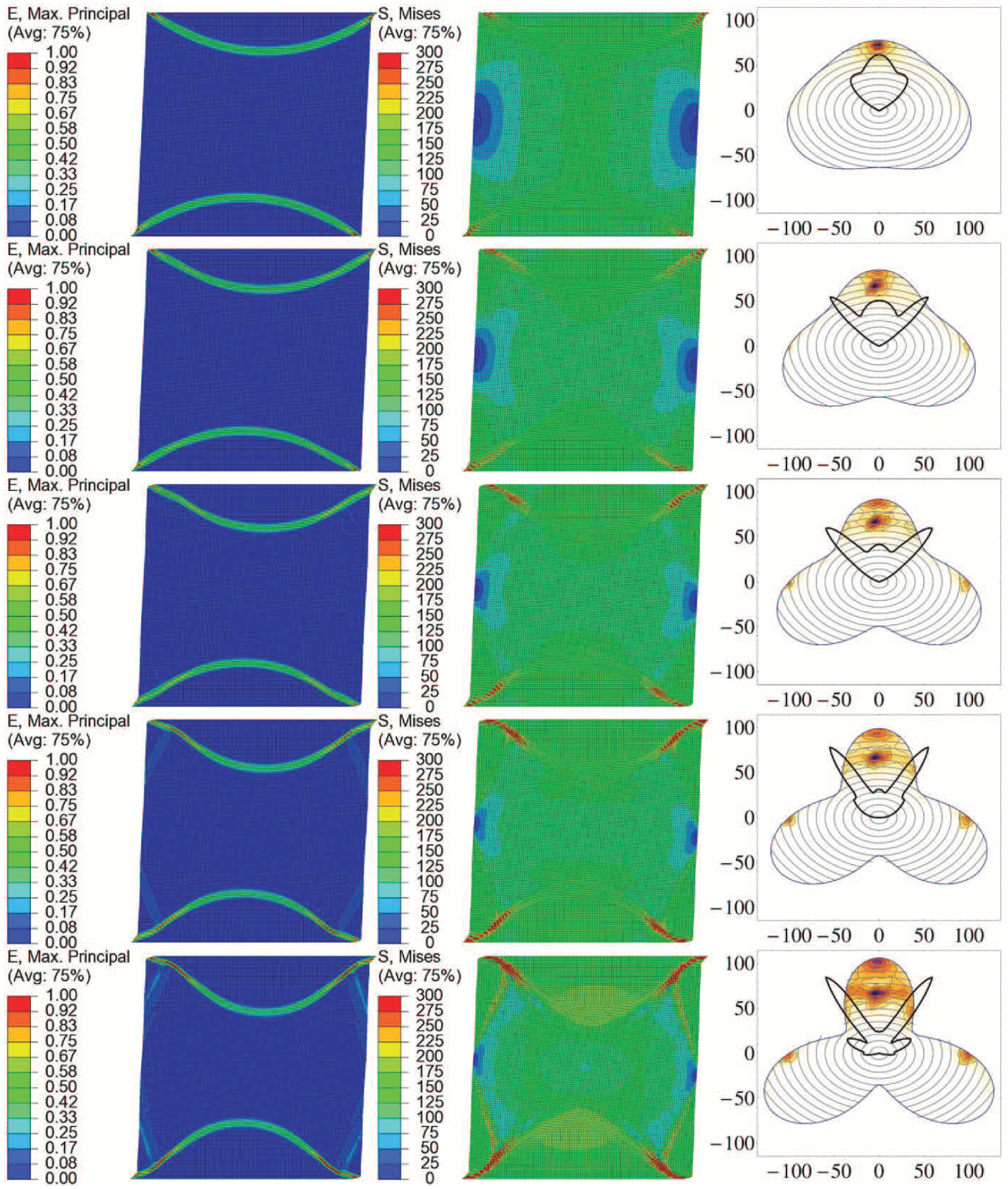
Upon putting bumps on the yield surface as described in Section 3.2, with positive values for a, we increase the yield stress in the direction of the predominant stress state and at ±120 with respect to this direction in the polar plane, see Figure 7. As a result, two stress concentrations develop in the two bulges that correspond not to the $T_{12}$ shear direction. The behaviour is more pronounced for larger values of a. The stress concentrations in the of- $T_{12}$ -shear bulges lie on the yield surface. One can see that the biggest part of the accumulated plastic deformation is produced on these, as their yield surface normals correspond very well to the largest parts of accumulated strain. The former predominant shear stress remains in the elastic region instead of following the extending yield surface. Only a small part of the original parallel shear band remains, and the overall plastic deformation is built up by a zig-zag pattern of shear bands that are of the $T_{12}$ -direction.

5.3. Non-convex yield surface 2: Reducing the yield stress in the $T_{12}$ -direction

In this case, the predominant shear stress state from the reference model is pushed to smaller levels, while offering larger elastic ranges in directions at ± 60 to this direction; see Figure 6. In fact, the former predominant stress is split into two predominant stress states that move to the adjacent of- $T_{12}$ -bulges on the yield surface as their amplitude is increased. The accumulated strains are noticeably parallel to the yield surface normals at the points of the stress concentrations, but the large nose in the $T_{12}$ -direction stems apparently from superposition of the two new predominant flow directions. Concurrently with this, the plastic deformation does not concentrate any more in the two parallel shear bands like in the reference solution; instead, a complex and laminate-like deformation pattern develops.

Figure 6.

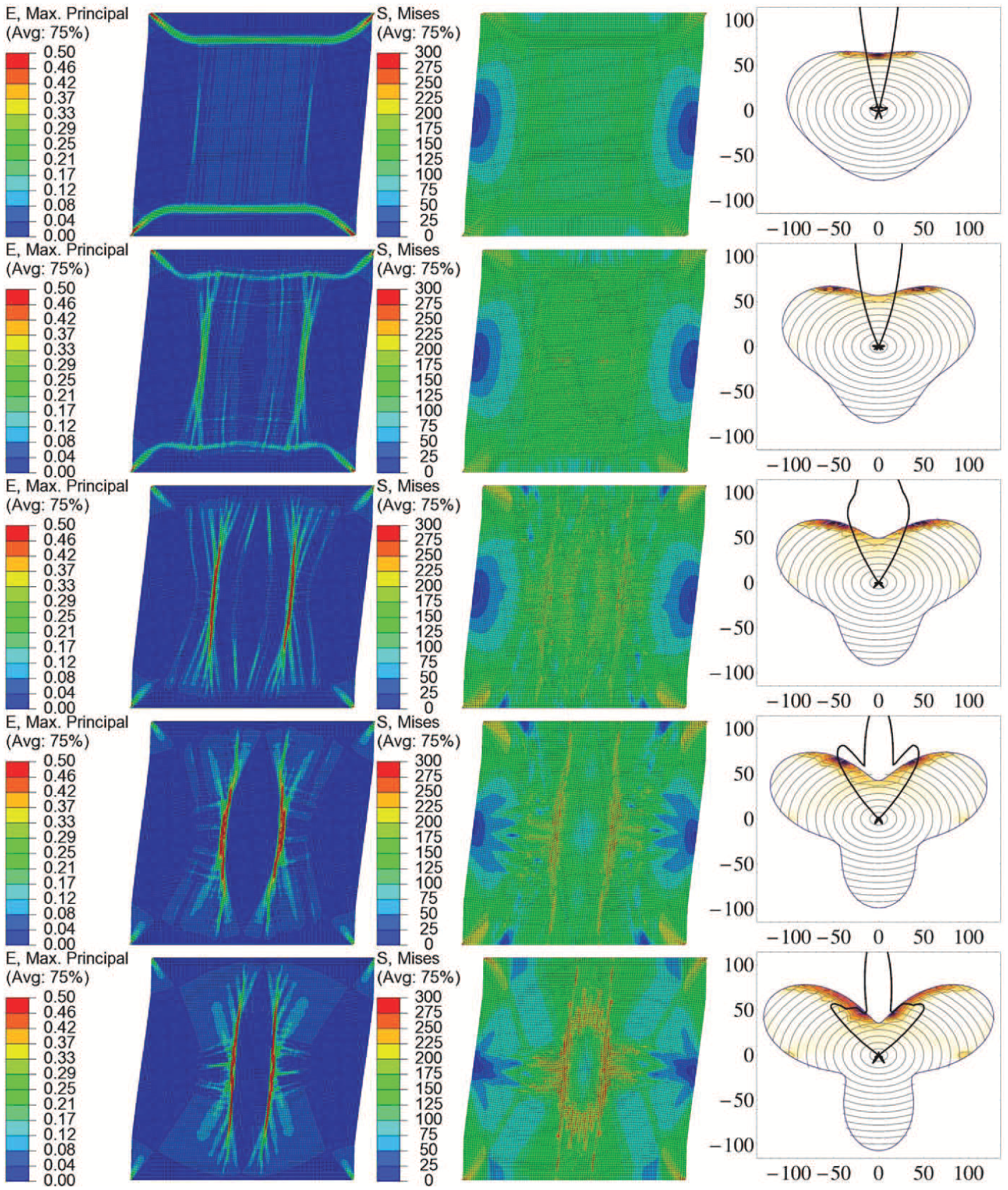
Simulations with a = {0.1, 0.2, 0.3, 0.4, 0.5} from the top to the bottom row. Left: Largest absolute strain eigenvalue from 0 (blue) to 0.5 (red). Centre: Equivalent von Mises stress from 0 (blue) to 300 MPa (red). Right: Elastic range projected perpendicular to the hydrostatic axis, where $(T_{22} - T_{11}) / \sqrt{2}$ and $T_{12}$ are drawn along the horizontal and vertical axes, respectively. The colour map indicates the density histogram of all stress states encountered in the finite element model at the end of the loading. The black line is a radial histogram of the accumulated plastic deformation. The elliptic isolines indicate the Mises stress levels in multiples of 10 MPa. As the absolute values depend strongly on the meshing and the statistical parameters, the histograms give only a qualitative impression of the stress and strain distributions at the end of the loading.

Figure 7.

Simulations with a ={–0.1, –0.2, –0.3, –0.4, –0.5} from the top to the bottom row. Left: Largest absolute strain eigenvalue from 0 (blue) to 1 (red). Centre: Equivalent von Mises stress from 0 (blue) to 300 MPa (red). Right: Elastic range projected perpendicular to the hydrostatic axis, where $(T_{22} - T_{11}) / \sqrt{2}$ and $T_{12}$ are drawn along the horizontal and vertical axes, respectively. The colour map indicates the density histogram of all stress states encountered in the finite element model at the end of the loading. The black line is a radial histogram of the accumulated plastic deformation. The elliptic isolines indicate the Mises stress levels in multiples of 10 MPa. As the absolute values depend strongly on the meshing and the statistical parameters, the histograms give only a qualitative impression of the stress and strain distributions at the end of the loading.

5.4. Cyclic loading

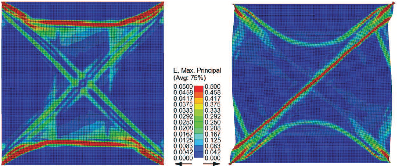
In this section, we examine the effect of the yield function on the residual of strain localization patterns in cyclic strain processes. The simulations from the preceding sections are repeated with a rigid displacement (0,0) →(0,0.05) →(0.05,0.05) →(0.05,0) →(0,0) with respect to $e_{1}$ and $e_{2}$ of the upper edge of the square sample, while the lower one is kept fixed. Comparing the plastic strain patterns at the end of the cycle for the isotropic reference model (a=0) and the non-convex model a = 0.5, we see no qualitative difference in the results, but there is a quantitative difference; see Figure 8. In both cases we have similar strain band patterns, but the remaining plastic strains are approximately 10 times larger in case of the non-convex yield function.

Figure 8.

Residual plastic strain after a cyclic loading (largest strain eigenvalue) on the left for the isotropic Mises material (colour map from 0 (blue) to 0.05 (red)) and on the right for the material with a = 0.5 (colour map from 0 (blue) to 0.5 (red)).

5.4.1. Simulations close to the point of loss of convexity

To look further for some qualitative change, we repeated the cyclic simulations with $a_{\pm}^{+}$ ≈ 1/19 ± 0.0025 and $a_{\pm}^{-}$ ≈-1/19 ± 0.0025, in other words, we consider two very similar yield surfaces, but one of them is convex while the other is not. This is done for both convexity limits ± 1/19 of a. It turns out that the results are virtually indistinguishable in both cases (no illustrations are provided, the results are very similar to the plots in Figure 8). Thus, it appears that the point of loss of convexity does not play a role as a bifurcation point.

6. Conclusions

We have set up a two-dimensional von Mises elastic–plastic material model in conjunction with a simple initial and boundary value problem. We modified the material model by putting bumps on the yield surface, preserving insensitivity to hydrostatic pressure. The modified model displays a non-convex but star-convex and anisotropic yield function.

In all simulations, including the cases of isotropic Mises materials, patterns of strain localization emerged. The complexity of the patterns and the local strain magnitude are loosely related to the bump amplitude. This behaviour appears to stem from the material anisotropy. Apart from that, no qualitative change of material behaviour could be attributed to the loss of convexity. This hypothesis is strenghtened by the fact that simulations of a circular deformation process with bump amplitudes just below and above the points of loss of convexity gave virtually indistinguishable results. Whether the situation is different in the three-dimensional case is open. To us it appears unlikely that the convexity of the yield function reflects a material property in the three-dimensional case but not in the two-dimensional case. To answer this question, the present analysis may be extended to the 3D case.

Footnotes

Funding

The author(s) disclosed receipt of the following financial support for the research, authorship, and/or publication of this article: Rainer Glüge received funding by the European research council under grant no. 4034011000. Sara Bucci received funding by the DFG (German research foundation) under grant no. GRK1554/2.

References

Drucker

On the postulate of stability of material in the mechanics of continua. J Méc 1964; 3: 235–249.

Krawietz

Stability and plastic yield of hypo-elastic materials. Habilitation Thesis, Technische Universität Berlin, Germany, 1979. Habilitation thesis.

Green

Naghdi

PM.

A general theory of an elastic-plastic continuum. Arch Rat Mech Anal 1965; 18: 251–281.

Kim

Oden

Generalized flow potentials in finite elastoplasticity II: Examples. Int J Eng Sci 1985; 23(5): 515–530.

Justusson

Phillips

Stability and convexity in plasticity. Acta Mechanica 1966; 2: 251–267.

Krawietz

Materialtheorie. Berlin: Springer, 1986.

Naghdi

. Stress-strain relations in plasticity and thermoplasticity. In: Proceedings of the Second Symposium on Naval Structural Mechanics. Oxford: Pergamon Press, 1960, 121–169.

Wilkins

Streit

Reaugh

Cumulative-strain-damage model of ductile fracture: Simulation and prediction of engineering fracture tests. Technical Report UCRL-53058, Lawrence Livermore Laboratory, University of California, CA, 1980.

Dannemeyer

Zur Veränderung der Fliefläche von Baustahl bei mehrachsiger plastischer Wechselbeanspruchung. PhD Thesis, Technische Universität Braunschweig, Germany, 1999.

10.

Ortiz

Repetto

Nonconvex energy minimization and dislocation structures in ductile single crystals. J Mech Phys Solid 1999; 47: 397–462.

11.

Kraska

Textursimulation bei groen inelastischen Verformungen mit der Technik des repräsentativen Volumenelements (RVE). PhD Thesis, TU Berlin, Germany, 1998.

12.

Miehe

Schotte

Lambrecht

Homogenization of inelastic solid materials at finite strains based on incremental minimization principles: Application to the texture analysis of polycrystals. J Mech Phys Solid 2002; 50(10): 2123–2167.

13.

Glüge

Weber

Bertram

Comparison of spherical and cubical statistical volume elements with respect to convergence, anisotropy, and localization behavior. Comput Mater Sci 2012; 63: 91–104.

14.

Glüge

Generalized boundary conditions on representative volume elements and their use in determining the effective material properties. Comput Mater Sci 2013; 79: 408–416.

15.

Kraska

Bertram

Simulation of polycrystals using an FEM-based representative volume element. Tech Mech 1996; 16(1): 51–62.

16.

Simo

Hughes

Computational inelasticity. New York, NY: Springer-Verlag, 1998.

17.

Dunne

Petrinic

Introduction to computational plasticity. Oxford: Oxford University Press, 2009.

18.

Alfano

De Angelis

Rosati

. A numerical algorithm for plane stress elastoplasticity. In: Owen

Oate

Hinton

(eds.) Computational plasticity: Fundamentals and applications (Proceedings of the Fifth International Conference on Computational Plasticity). Barcelona, Spain: CIMNE International Center for Numerical Methods in Engineering, 343–348.

19.

Pedroso

Sheng

Sloan

Stress update algorithm for elastoplastic models with nonconvex yield surfaces. Int J Numer Meth Eng 2008; 76(13): 2029–2062.