Solution of contact problems for Gao beam and elastic foundation

Abstract

This paper presents mathematical formulations and a solution for contact problems that concern the nonlinear beam published by Gao (Nonlinear elastic beam theory with application in contact problems and variational approaches, Mech Res Commun 1996; 23: 11–17) and an elastic foundation. The beam is subjected to a vertical and also axial loading. The elastic deformable foundation is considered at a distance under the beam. The contact is modeled as static, frictionless and using the normal compliance contact condition. In comparison with the usual contact problem formulations, which are based on variational inequalities, we are able to derive for our problem a nonlinear variational equation. Solution of this problem is realized by means of the so-called control variational method. The main idea of this method is to transform the given contact problem to an optimal control problem, which can provide the requested solution. Finally, some results including numerical examples are offered to illustrate the usefulness of the presented solution method.

Keywords

Nonlinear beam Winkler foundation contact problem normal compliance condition control variational method finite element method

1. Introduction

Contact problems are generally very important in practice. However they are quite difficult and the difficulties arise mainly from the fact that the contact domain is unknown a priori and should be determined during a solution process.

This study is going to deal with the nonlinear beam model developed by Gao and an elastic foundation, which are in possible contact. It is well known that the contact of elastic bodies may be modeled using the Signorini conditions, when the obstacle is rigid, and that leads to formulations with variational inequalities [1]. If the contact is modeled with a normal compliance condition, we can obtain the mathematical description for problems with deformable obstacle, and this description has a form of nonlinear equation. In Gao et al. [2] the Gao beam resting on a deformable foundation was studied. More about normal compliance conditions can be found for instance in Shillor et al. [3] or Sofonea and Matei [1].

Solving such equations, one may find the so-called control variational method to be very useful. The method was introduced in Arnautu et al. [4] and Sprekels and Tiba [5] as a new interesting method for analyzing and solving differential equations. It is remarkable both from the theoretical and the numerical points of view. Later it was used in the study of various problems [6, 7], but from our point of view, two papers, Sofonea and Tiba [8] and Barboteu et al. [9] are important, as they describe the contact of a cantilever Euler–Bernoulli beam with an obstacle. More applications concerning the control variational method are given in the monograph by Neittaanmäki et al. [10].

Using this method. the functional of total potential energy is transformed in such a way that it is possible to formulate an optimal control problem governed by the Euler–Bernoulli beam equation. The nonlinear terms from the variational equation are fully included in the control variable. Afterwards one can solve the resulting optimal control problem to obtain a solution of the original contact problem.

The aim of this paper is to generalize this idea for nonlinear beam and arbitrary boundary conditions. We are also going to extend considerably the results of our previous article [11] but only the convex case will be considered here.

It should be noted that a convex potential energy means that the static system has a unique solution, whereas a nonconvex potential energy leads to buckling phenomena, when the system has three solutions. In contrast, it is remarkable that the dynamic problems with the normal compliance condition always have a unique solution. Several interesting studies of such problems have already been published. Dynamic contact of the Gao beam with a reactive or rigid foundation is analyzed and computed in Andrews et al. [12, 13], the problem of two coupled Gao beams connected via a joint with a gap is described in Ahn et al. [14].

2. Nonlinear beam model by Gao

The most-used beam model is still the linear model by Euler and Bernoulli, which was established in about 1750. Nowadays its bending problem can be solved quite easily using the Finite Element Method (FEM) see Reddy [15], but in fact it does not allow greater deflections than very small ones compared to its length. There exist numerous nonlinear beam models. We think that one of the most interesting is the mathematical model proposed in 1996 by D. Y. Gao [16], which respects the original Euler–Bernoulli hypothesis, i.e. straight lines normal to the mid-surface remain straight and normal to the mid-surface after deformation, and at the same time enables moderately large deflections. Its advantage consists of its relative simplicity and good possibilities for a post-buckling analysis.

The governing equation for the Gao beam reads as follows

EI w^{''''} - Eα {(w^{'})}^{2} w^{″} + Pμ w^{″} = f in (0, L),

(1)

where we denote

I = \frac{2}{3} h^{3} b, α = 3 hb (1 - ν^{2}), μ = (1 + ν) (1 - ν^{2}), f = (1 - ν^{2}) q,

(2)

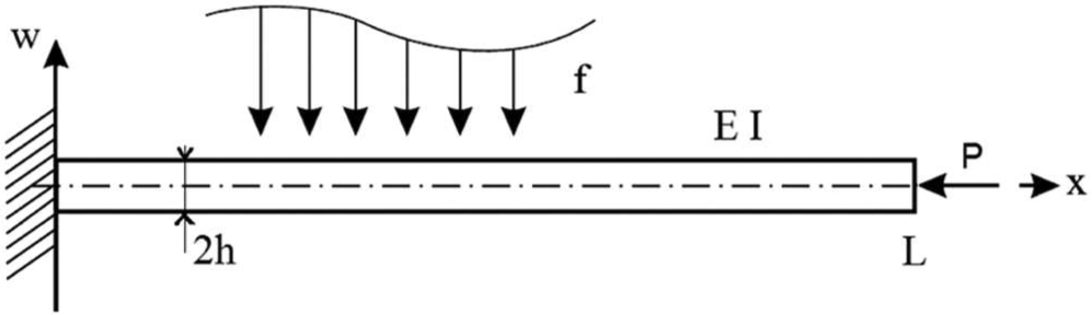
E is the elastic modulus of the material, I is the area moment of inertia of the beam’s cross-section, w is the transverse displacement of the beam, $ν$ is the Poisson’s ratio, P is the axial force acting at the point $x = L$ , q is the distributed vertical load, $2 h$ and $L$ represent the height and length of the beam respectively and its width $b$ is considered as a unit (Figure 1).

Figure 1.

Nonlinear beam by Gao.

Naturally, there exists the functional of the potential energy for this beam model. First let us specify the function spaces that will be used in connection with this functional.

Throughout this paper we will consider four fundamental boundary value problems with corresponding function spaces $V_{i}, i = 1, 2, 3, 4$ . They are as follows:

(P1): clamped (or fixed) beam

$V_{1} = {v \in H^{2} ((0, L)) : v (0) = v^{'} (0) = 0, v (L) = v^{'} (L) = 0}$ ,

(P2): propped cantilever beam

$V_{2} = {v \in H^{2} ((0, L)) : v (0) = v^{'} (0) = 0, v (L) = 0}$ ,

(P3): cantilever beam

$V_{3} = {v \in H^{2} ((0, L)) : v (0) = v^{'} (0) = 0}$ ,

(P4): simply supported beam

$V_{4} = {v \in H^{2} ((0, L)) : v (0) = 0, v (L) = 0}$ .

Next V will be any of the above-mentioned spaces $V_{1}, \dots, V_{4}$ . Let us introduce three bilinear forms

\begin{matrix} a (w, v) = \int_{0}^{L} EI w^{″} v^{″} dx, d (w, v) = \int_{0}^{L} Pμ w^{'} v^{'} dx, w, v \in V, \end{matrix}

(3)

\begin{matrix} b (w, v) = a (w, v) - d (w, v), w, v \in V, \end{matrix}

(4)

together with the following notations

(w, v) = \int_{0}^{L} wv dx, π (w, v) = \frac{1}{3} \int_{0}^{L} Eα {(w^{'})}^{3} v^{'} dx, w, v \in V .

(5)

Using this notation we define

\begin{matrix} Π_{0} (v) = \frac{1}{2} a (v, v) - (f, v) = \frac{1}{2} \int_{0}^{L} EI {(v^{″})}^{2} dx - \int_{0}^{L} fv dx, \end{matrix}

(6)

\begin{matrix} Π_{N} (v) = \frac{1}{4} π (v, v) = \frac{1}{12} \int_{0}^{L} Eα {(v^{'})}^{4} dx, \end{matrix}

(7)

\begin{matrix} Π_{P} (v) = - \frac{1}{2} d (v, v) = - \frac{1}{2} \int_{0}^{L} Pμ {(v^{'})}^{2} dx . \end{matrix}

(8)

Then the functional of the potential energy for the Gao beam can be expressed as follows

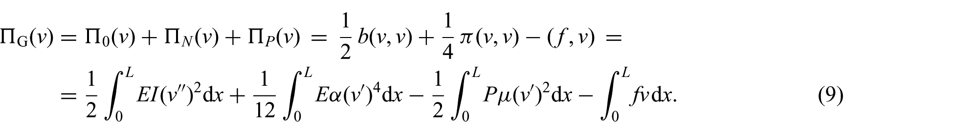
\begin{matrix} Π_{G} (v) = Π_{0} (v) + Π_{N} (v) + Π_{P} (v) = \frac{1}{2} b (v, v) + \frac{1}{4} π (v, v) - (f, v) = \\ = \frac{1}{2} \int_{0}^{L} EI {(v^{″})}^{2} dx + \frac{1}{12} \int_{0}^{L} Eα {(v^{'})}^{4} dx - \frac{1}{2} \int_{0}^{L} Pμ {(v^{'})}^{2} dx - \int_{0}^{L} fv dx . \end{matrix}

(9)

It is easy to verify, that every stationary point w of $Π_{G}$ , i.e. $w \in V$ such that

Π_{G}^{'} (w, v) = 0 \forall v \in V,

(10)

where $Π_{G}^{'} (w, v)$ is the Gâteaux differential of $Π_{G}$ at w in the direction v, satisfies following nonlinear equation

b (w, v) + π (w, v) = (f, v) \forall v \in V .

(11)

In the case where w is a sufficiently smooth function, it satisfies also equation (1), which can under this assumption be easily derived from equation (11).

Finally, we associate with the functional (9) the following variational problem

\{\begin{matrix} Find w \in V such that \\ Π_{G} (w) = min_{v \in V} Π_{G} (v) . \end{matrix}

(12)

Then we need to establish conditions of existence and uniqueness for the solution of equation (12) together with its relation to equation (11).

It is evident that generally the functional $Π_{G}$ is not convex, which is caused by the term $Π_{P}$ . Following the classic beam theory, the Euler critical load can be determined for the Gao beam by

P_{cr}^{E} = min_{v \in V} \frac{\int_{0}^{L} EI {(v^{″})}^{2} dx}{\int_{0}^{L} μ {(v^{'})}^{2} dx} .

(13)

From this definition we have

\int_{0}^{L} EI {(v^{″})}^{2} dx \geq P \int_{0}^{L} μ {(v^{'})}^{2} dx \forall v \in V, \forall P \leq P_{cr}^{E} .

(14)

Thereafter it can be proved that $Π_{G}$ is strictly convex on V for any axial load that is less than the critical value $P_{cr}^{E}$ . To prove it we need to show that for any $w \in V$

Π_{G}^{′′} (w, v, v) = b (v, v) + \int_{0}^{L} Eα {(w^{'})}^{2} {(v^{'})}^{2} dx > 0 \forall v \in V, v \neq 0 .

(15)

However the integral in equation (15) is always nonnegative and from equation (14) we obtain under assumption $P < P_{cr}^{E}$ that $b (v, v) > 0$ for any $v \in V, v \neq 0$ , hence equation (15) is valid.

Moreover, $Π_{G}$ is coercive on V for any load P. It is easy to prove that there exist constant $\hat{c} > 0$ such that

∥ {(v^{'})}^{2} ∥_{L^{2}} \geq \hat{c} ∥ v^{'} ∥_{L^{2}}^{2} \forall v \in H^{1} ((0, L)) .

(16)

Using the Friedrichs’ inequality for $a (v, v)$ together with equation (16) we get

Π_{G} (v) \geq (c_{1} ∥ v ∥_{H^{2}} - ∥ f ∥) ∥ v ∥_{H^{2}} + (c_{2} ∥ v^{'} ∥_{L^{2}}^{2} + c_{3}) ∥ v^{'} ∥_{L^{2}}^{2} \forall v \in H^{2} ((0, L)) .

(17)

The constants $c_{1}, c_{2}$ are positive, and c₃ has the opposite sign to the force P. From equation (17) we immediately obtain for arbitrary value P the coercivity condition

∥ v ∥_{V} \to + \infty \Rightarrow Π_{G} (v) \to + \infty .

(18)

Now taking into consideration, that $Π_{G}$ is continuous on V, as a result we obtain the existence and uniqueness for the solution of equation (12) and its equivalence to equation (11).

As $P_{cr}^{E}$ is a positive value, for $P < 0$ equation (12) has exactly one solution. If $P > 0$ , which means a compression of the beam, the situation is more complicated as the functional $Π_{G}$ can be nonconvex. The limit value, where convexity of $Π_{G}$ changes to nonconvexity, is for a Gao beam generally somewhat larger than the Euler value given by equation (13). Unfortunately, this critical point $P_{cr}$ cannot be expressed using a formula and only numerical experiments can give us an approximate value. For $P > P_{cr}$ Gao demonstrated in Gao and Ogden [17] that $Π_{G}$ has three stationary points: two local minimizers and one local maximizer.

Let us recall that in this paper only the convex case will be considered.

3. Contact problems with a deformable foundation

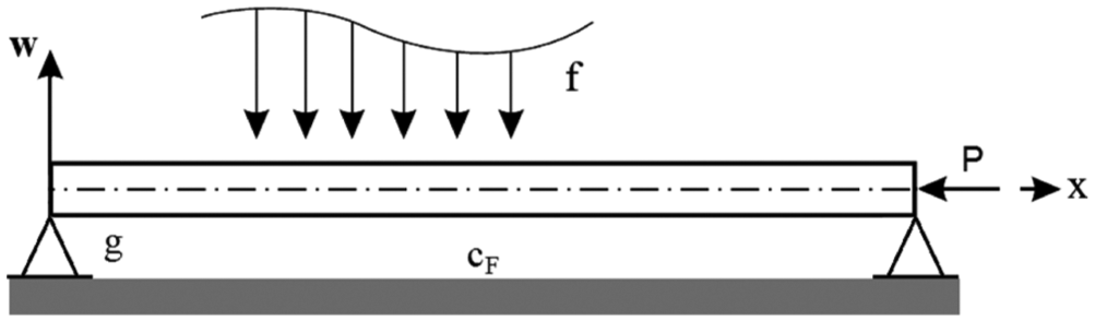
Previous considerations will be now extended to contact problems, where the beam is situated above a foundation. The gap between them is described by the function $g \leq 0$ and for simplicity this function will be considered constant. The foundation is assumed to be deformable and governed by the Winkler one-parametric model with a foundation modulus $k_{F}$ .

After that, the beam equation (1) is modified in the following way

EI w^{′′′′} - Eα {(w^{'})}^{2} w^{″} + Pμ w^{″} = f + T (w) in (0, L),

(19)

where

T (w) = c_{F} {(g - w)}^{+}, c_{F} = (1 - ν^{2}) k_{F},

(20)

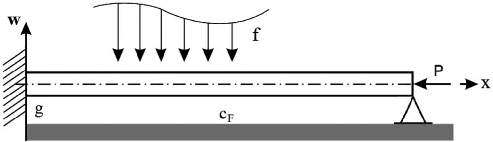
represents contact forces between the beam and the foundation (Figure 2), $T (w) = 0$ if there is no contact. Such a description belongs to contact problem formulations with normal compliance contact conditions [1, 3].

Figure 2.

Beam and foundation.

Next we will establish a variational formulation of the considered contact problem. First let us introduce the energy of reaction forces resulting from beam–foundation interaction by

Π_{F} (v) = \frac{1}{2} \int_{0}^{L} c_{F} {({(g - v)}^{+})}^{2} dx

(21)

together with a nonlinear form

\begin{matrix} κ (w, v) = \int_{0}^{L} c_{F} {(g - w)}^{+} v dx, w, v \in V . \end{matrix}

(22)

The total energy is then given by the sum of equations (9) and (21):

Π_{T} (v) = Π_{G} (v) + Π_{F} (v) = \frac{1}{2} b (v, v) + \frac{1}{4} π (v, v) + Π_{F} (v) - (f, v) .

(23)

Using the same arguments as above we can prove for $Π_{T}$ coercivity on V and strict convexity for all axial loads $P < P_{cr}^{E}$ . Again, the value $P_{cr}^{E}$ is here not the critical or limit value $P_{cr}$ , but we are not able to specify it exactly as the situation is now even more complicated than before due to an effect of potential contact.

Let us define the following minimization problem

\{\begin{matrix} Find w \in V such that \\ Π_{T} (w) = min_{v \in V} Π_{T} (v) . \end{matrix}

(24)

From the convexity and coercivity of $Π_{T}$ it can be argued that

Equation (24) has exactly one solution for arbitrary $f \in L^{2} ((0, L))$ and any $P < P_{cr}^{E}$ .

This solution is also the unique solution of the following nonlinear equation

\{\begin{matrix} Find w \in V such that \\ b (w, v) + π (w, v) - κ (w, v) = (f, v) \forall v \in V, \end{matrix}

(25)

which characterizes the stationary point of $Π_{T}$ .

4. Solution using the control variational method

The main idea of the control variational method is to perform a minimization of the energy functional via an optimal control problem. Hence the optimal control theory plays an essential role in this approach. It is briefly described in the Appendix.

Changing the original problem to another one can be regarded as a transformation of variational principles, see Kravchuk and Neittaanmäki [18]. Many mathematical problems are solved using transformations. The idea is to transform the problem into another one we know how to solve. Of course, we have to prove that by means of solving the transformed problem we obtain a solution of the original one.

4.1. Transformation T1

In this section we will deal with transformation of variational problems which is sometimes called Friedrichs’ transformation, see Kravchuk and Neittaanmäki [18], chapter 5. Such an approach involves, for example, declaring the function v and its derivative $v^{'}$ to be independent arguments of the given functional.

Following this idea, let us define in equation (23) a new variable: $z = v^{'}$ .

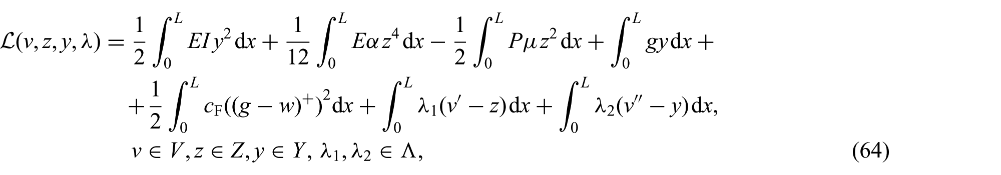
This way we transform the functional (23) from equation (24) into a Lagrangian $L$ , because the relation $z = v^{'}$ can be understood as a constraint. Taking $λ$ as a Lagrange multiplier corresponding to this constraint, we obtain

\begin{matrix} L (v, z, λ) = \frac{1}{2} \int_{0}^{L} EI {(v^{″})}^{2} dx + \frac{1}{12} \int_{0}^{L} Eα z^{4} dx - \frac{1}{2} \int_{0}^{L} Pμ z^{2} dx - \int_{0}^{L} fv dx + \\ + \frac{1}{2} \int_{0}^{L} c_{F} {({(g - w)}^{+})}^{2} dx + \int_{0}^{L} λ (v^{'} - z) dx, v \in V, z \in Z, λ \in Λ, \end{matrix}

(26)

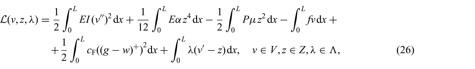
where V is an appropriate Sobolev space, Z denotes space containing derivatives of functions from V and $Λ = L^{2} ((0, L))$ . As a result, we obtain from equation (24) the following saddle-point problem for Lagrangian (26)

L (v, z, λ) \to \underset{v, z, λ}{stat} .

(27)

Equations for the saddle point $(w, \bar{z}, \bar{λ})$ can be acquired using the stationary point equations for $L$ . They are obtained by setting the variations of this functional to zero. For better readability we will not write $\bar{z}, \bar{λ}$ , but only $z, λ$ .

\begin{matrix} \int_{0}^{L} EI w^{″} φ^{″} dx - \int_{0}^{L} fφ dx - \int_{0}^{L} c_{F} {(g - w)}^{+} φ dx + \int_{0}^{L} λ φ^{'} dx = 0 \forall φ \in V, \end{matrix}

(28)

\begin{matrix} \frac{1}{3} \int_{0}^{L} Eα z^{3} φ dx - \int_{0}^{L} Pμ zφ dx - \int_{0}^{L} λφ dx = 0 \forall φ \in Z, \end{matrix}

(29)

\begin{matrix} \int_{0}^{L} (w^{'} - z) φ dx = 0 \forall φ \in Λ . \end{matrix}

(30)

For any possible boundary conditions we have $φ (0) = 0$ , hence

\int_{0}^{L} λ φ^{'} dx = - \int_{0}^{L} λ^{'} φ dx + (λφ) (L) \forall φ \in V .

(31)

This implies condition

(λφ) (L) = 0,

(32)

what is trivially satisfied for boundary problems (P1), (P2)and (P4).

Next let us define a new variable u by means of the following equation

\int_{0}^{L} uφ dx = \int_{0}^{L} λ^{'} φ dx + \int_{0}^{L} c_{F} {(g - w)}^{+} φ dx \forall φ \in V .

(33)

Equations (in classical form) for a stationary point are then as follows

\begin{matrix} EI w^{′′′′} = f + u, \end{matrix}

(34)

\begin{matrix} u = λ^{'} + c_{F} {(g - w)}^{+}, \end{matrix}

(35)

\begin{matrix} \frac{1}{3} Eα z^{3} - Pμ z = λ, \end{matrix}

(36)

\begin{matrix} w^{'} = z . \end{matrix}

(37)

Furthermore, from equations (28) and (33) we can get

a (w, v) = (f, v) + (u, v) \forall v \in V .

(38)

Let $\hat{w} \in V$ be the solution of equation (38) with $u = 0$ , i.e.

a (\hat{w}, v) = (f, v) \forall v \in V .

(39)

Obviously, such a solution exists and is unique. Then we can rewrite the functional (6) with regard to equations (38) and (39) as follows

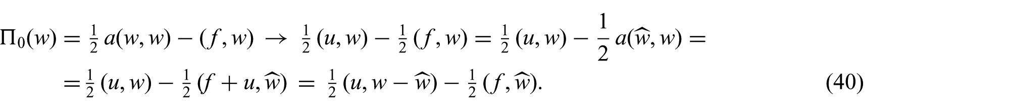
\begin{matrix} Π_{0} (w) = \frac{1}{2} a (w, w) - (f, w) \to \frac{1}{2} (u, w) - \frac{1}{2} (f, w) = \frac{1}{2} (u, w) - \frac{1}{2} a (\hat{w}, w) = \\ = \frac{1}{2} (u, w) - \frac{1}{2} (f + u, \hat{w}) = \frac{1}{2} (u, w - \hat{w}) - \frac{1}{2} (f, \hat{w}) . \end{matrix}

(40)

Now it is possible to transform the functional (23). Using equation (40) we get

\begin{matrix} Π_{T} (w) = \frac{1}{2} b (w, w) + \frac{1}{4} π (w, w) + Π_{F} (w) - (f, w) \to \\ \to & \frac{1}{2} (u, w - \hat{w}) + \frac{1}{4} π (w, w) - \frac{1}{2} d (w, w) + Π_{F} (w) - \frac{1}{2} (f, \hat{w}) . \end{matrix}

(41)

The last term in equation (41) is evidently constant and therefore it may be omitted during minimization. This way we finally obtain the transformed form of the functional $Π_{T}$ as follows

\begin{matrix} J_{1} (w, u) = \frac{1}{2} \int_{0}^{L} u (w - \hat{w}) dx + \frac{1}{12} \int_{0}^{L} Eα {(w^{'})}^{4} dx - \frac{1}{2} \int_{0}^{L} Pμ {(w^{'})}^{2} dx + \\ + \frac{1}{2} \int_{0}^{L} c_{F} {({(g - w)}^{+})}^{2} dx, \end{matrix}

(42)

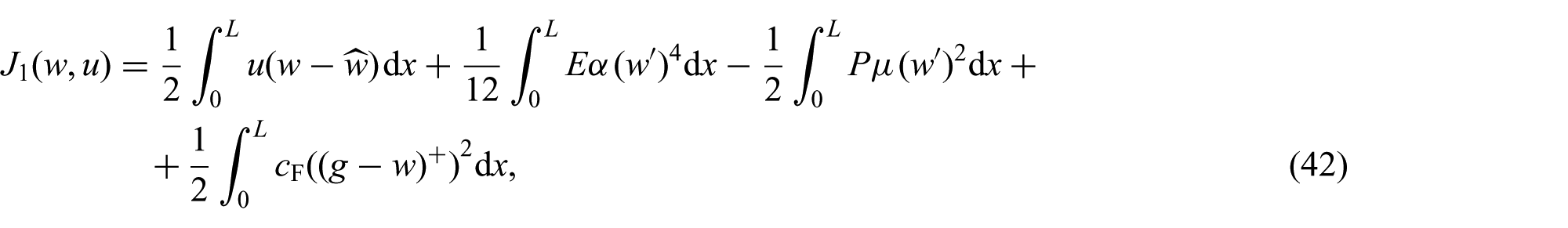
where the function $\hat{w}$ solves equation (39).

4.2. Contact problem solution by means of transformation T1

As a result of the previous paragraph considerations we obtained by means of equations (38) and (41) the following optimal control problem

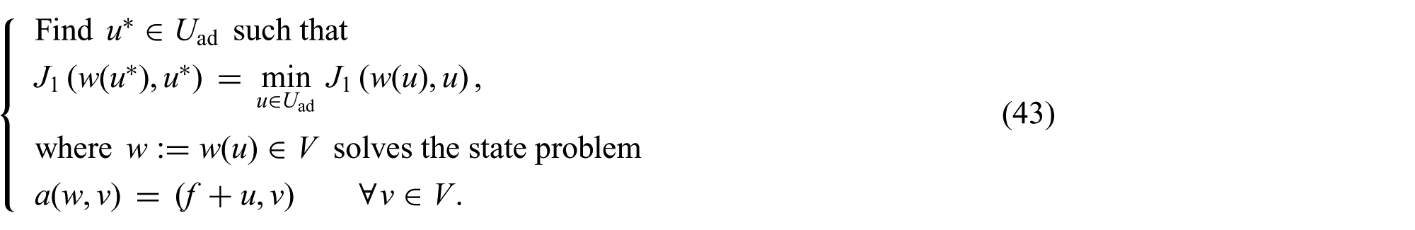
\{\begin{matrix} Find u^{*} \in U_{ad} such that \\ J_{1} (w (u^{*}), u^{*}) = min_{u \in U_{ad}} J_{1} (w (u), u), \\ where w : = w (u) \in V solves the state problem \\ a (w, v) = (f + u, v) \forall v \in V . \end{matrix}

(43)

The set of admissible controls is defined by

U_{ad} = {u \in L^{2} ((0, L)) : | u (x) | \leq C a.e. in (0, L)},

(44)

where $C > 0$ is a constant, V is any of the spaces $V_{1}, \dots, V_{4}$ and $\hat{w}$ is given by equation (39).

First we need to know conditions concerning the existence of a solution for our problem (43).

Theorem 1. Problem (43) has under the assumption $P < P_{cr}^{E}$ exactly one solution.

Proof: The state equation is here nothing but the classical Euler–Bernoulli equation, hence the existence and uniqueness of its solution is guaranteed. We express from equation (38) the unknown u by

(u, v) = a (w, v) - (f, v) \forall v \in V

(45)

and substitute it into equation (42). Using equation (39) we get

\begin{matrix} J_{1} (w, u) = \frac{1}{2} (u, w) - \frac{1}{2} (u, \hat{w}) + \frac{1}{4} π (w, w) - \frac{1}{2} d (w, w) + Π_{F} (w) \to \\ \to \frac{1}{2} a (w, w) + \frac{1}{4} π (w, w) - \frac{1}{2} d (w, w) - (f, w) + Π_{F} (w) + \frac{1}{2} (f, \hat{w}) . \end{matrix}

(46)

This is, up to the last term, which is constant, the functional $Π_{T}$ . We already know that under the assumption $P < P_{cr}^{E}$ it is strictly convex and coercive. Hence the minimization problem has the only solution $w^{*} \in V$ . To this function corresponds just one control value $u^{*}$ given according to equation (45) by

(u^{*}, v) = a (w^{*}, v) - (f, v) \forall v \in V .

(47)

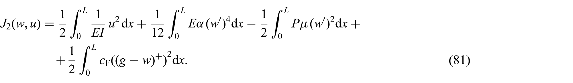
The optimal pair $(w^{*}, u^{*}) \in V \times U_{ad}$ for equation (43) therefore exists and is unique. $□$

Next we need to explain the relationship between the contact problem (24) and the optimal control problem (43).

Theorem 2. Let $f \in L^{2} ((0, L))$ and $P < P_{cr}^{E}$ . Let $u^{*}$ be a solution of equation (43). Then function $w^{*} : = w (u^{*})$ is a solution of the associated problem (24) under the assumption that the constant C in equation (44) is sufficiently large.

Proof: Here we will follow the idea of the proof from Sofonea and Tiba [8], where an analogous theorem was proved.

The existence of an optimal pair $(w^{*}, u^{*}) \in V \times U_{ad}$ for equation (43) follows from Theorem 1 for any positive constant C.

Let now consider a feasible pair of the form

(w, u) = (w^{*} + t (y - w^{*}), u^{*} + t (z - u^{*}))

(48)

for any $t \in [- 1, 1]$ , $z \in U_{ad}$ a $y \in V$ satisfying the state equation (38):

a (w^{*} + t (y - w^{*}), v) = (f + u^{*} + t (z - u^{*}), v) \forall v \in V .

(49)

Because

a (w^{*}, v) = (f + u^{*}, v) \forall v \in V,

(50)

we get by comparing equations (49) and (50) that the pair $(y, z)$ must fulfill

a (y - w^{*}, v) = (z - u^{*}, v) \forall v \in V .

(51)

Substituting from equation (50) we obtain

a (y, v) = (f + z, v) \forall v \in V .

(52)

Optimality of the pair $(w^{*}, u^{*})$ implies

J_{1} (w^{*}, u^{*}) \leq J_{1} (w, u) \forall (w, u) \in V \times U_{ad},

(53)

hence

\begin{matrix} \frac{1}{2} (u^{*}, w^{*} - \hat{w}) + Π_{N} (w^{*}) + Π_{P} (w^{*}) + Π_{F} (w^{*}) \leq \\ \leq \frac{1}{2} (u, w - \hat{w}) + Π_{N} (w) + Π_{P} (w) + Π_{F} (w) \forall (w, u) \in V \times U_{ad} . \end{matrix}

(54)

Substitution from equation (48) leads after some rearrangement to

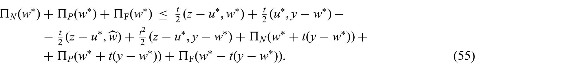
\begin{matrix} Π_{N} (w^{*}) + Π_{P} (w^{*}) + Π_{F} (w^{*}) \leq \frac{t}{2} (z - u^{*}, w^{*}) + \frac{t}{2} (u^{*}, y - w^{*}) - \\ - \frac{t}{2} (z - u^{*}, \hat{w}) + \frac{t^{2}}{2} (z - u^{*}, y - w^{*}) + Π_{N} (w^{*} + t (y - w^{*})) + \\ + Π_{P} (w^{*} + t (y - w^{*})) + Π_{F} (w^{*} - t (y - w^{*})) . \end{matrix}

(55)

Transposing all terms to the right-hand side, dividing this inequality by $t > 0$ and passing to the limit as $t \to 0$ we obtain using equations (50), (51) and (39)

\begin{matrix} 0 \leq \frac{1}{2} (z - u^{*}, w^{*}) + \frac{1}{2} (u^{*}, y - w^{*}) - \frac{1}{2} (z - u^{*}, \hat{w}) + Π_{N}^{'} (w^{*}, y - w^{*}) + \\ + Π_{P}^{'} (w^{*}, y - w^{*}) + Π_{F}^{'} (w^{*}, y - w^{*}) = \\ = a (w^{*}, y - w^{*}) - (f, y - w^{*}) + π (w^{*}, y - w^{*}) - d (w^{*}, y - w^{*}) - κ (w^{*}, y - w^{*}) \end{matrix}

(56)

for arbitrary pair $(y, z) \in V \times U_{ad}$ satisfying equation (52). Since the same can be applied for $t < 0$ , as a result we obtain equation (25), which is equivalent to the minimization problem (24). $□$

Finally let us determine the optimality conditions for the problem (43). Using the general results from the Appendix we get for an optimal pair $(w^{*}, u^{*}) \in V \times U_{ad}$ :

\begin{matrix} a (w^{*}, v) = (f + u^{*}, v) \forall v \in V, \end{matrix}

(57)

\begin{matrix} a (p^{*}, v) = \frac{1}{2} (u^{*}, v) + π (w^{*}, v) - d (w^{*}, v) - κ (w^{*}, v) \forall v \in V, \end{matrix}

(58)

\begin{matrix} (w^{*} + 2 p^{*}, u - u^{*}) & \geq & (\hat{w}, u - u^{*}) \forall u \in U_{ad} . \end{matrix}

(59)

Here $p^{*} \in V$ represents the adjoint state as it is a solution of the adjoint equation (58). Equation (57) is nothing but the state problem.

The previous solution procedure, which is based on using the transformation T1, is in some sense generic as it can be applied to every boundary problem (P1)–(P4). The state equation is here the classical Euler–Bernoulli equation of the fourth order.

An interesting idea leading to a different optimal control problem with the state equation of the second order was proposed in papers by Sofonea and Tiba [8] and Barboteu et al. [9], but only the cantilever beam for the Euler–Bernoulli model was considered there.

In the next section we will follow in a certain way the previous idea. For this purpose we introduce another transformation, as we need a more general approach than in the above-mentioned papers.

4.3. Transformation T2

This transformation is based on the definitions of two new variables and the concept of transformed loading

z = v^{'}, y = v^{″}, f \to g .

(60)

Of course, the function of transformed loading g still needs to be determined. To this end let us consider function $f \in L^{2} ((0, L))$ from equation (23) and let $g \in L^{2} ((0, L))$ be a function such that

\int_{0}^{L} g v^{″} dx = - \int_{0}^{L} fv dx \forall v \in V,

(61)

where V is the given space of test functions. If we can suppose that g lies in the space $H^{2} ((0, L))$ , it is quite natural to determine g by

- \int_{0}^{L} g^{″} v dx = \int_{0}^{L} fv dx \forall v \in V .

(62)

Using the Green formula we obtain from here that

- (g v^{'}) (L) + (g v^{'}) (0) + (g^{'} v) (L) = 0 \forall v \in V,

(63)

where we took into account that for every boundary problem, it holds that $v (0) = 0$ .

The transformation (60) converts the functional (23) through the use of transformed loading (61) to Lagrangian

\begin{matrix} L (v, z, y, λ) = \frac{1}{2} \int_{0}^{L} EI y^{2} dx + \frac{1}{12} \int_{0}^{L} Eα z^{4} dx - \frac{1}{2} \int_{0}^{L} Pμ z^{2} dx + \int_{0}^{L} gy dx + \\ + \frac{1}{2} \int_{0}^{L} c_{F} {({(g - w)}^{+})}^{2} dx + \int_{0}^{L} λ_{1} (v^{'} - z) dx + \int_{0}^{L} λ_{2} (v^{″} - y) dx, \\ v \in V, z \in Z, y \in Y, λ_{1}, λ_{2} \in Λ, \end{matrix}

(64)

and the problem of finding its saddle point. Here we use the same notation as before, in addition Y is a space containing second derivatives of functions from V.

The system of equations representing such a saddle point is as follows

\begin{matrix} - \int_{0}^{L} c_{F} {(g - w)}^{+} φ dx + \int_{0}^{L} λ_{1} φ^{'} dx + \int_{0}^{L} λ_{2} φ^{″} dx = 0 \forall φ \in V, \end{matrix}

(65)

\begin{matrix} \frac{1}{3} \int_{0}^{L} Eα z^{3} φ dx - \int_{0}^{L} Pμ zφ dx - \int_{0}^{L} λ_{1} φ dx = 0 \forall φ \in Z, \end{matrix}

(66)

\begin{matrix} \int_{0}^{L} EI yφ dx + \int_{0}^{L} gφ dx - \int_{0}^{L} λ_{2} φ dx = 0 \forall φ \in Y, \end{matrix}

(67)

\begin{matrix} \int_{0}^{L} (w^{'} - z) φ dx = 0 \forall φ \in Λ, \end{matrix}

(68)

\begin{matrix} \int_{0}^{L} (w^{″} - y) φ dx = 0 \forall φ \in Λ . \end{matrix}

(69)

Next we introduce the variable u by

\int_{0}^{L} uφ dx = - \int_{0}^{L} λ_{2} φ dx \forall φ \in Y .

(70)

Under the following two assumptions

(λ_{1} φ) (L) = 0 \forall φ \in V,

(71)

- (λ_{2}' φ) (L) + (λ_{2} φ^{'}) (L) - (λ_{2} φ^{'}) (0) = 0 \forall φ \in V,

(72)

we eliminate the unknown y by substituting $y = w^{″}$ from equation (69) into equation (67) and finally obtain

\begin{matrix} - u^{″} = {λ_{1}}^{'} + c_{F} {(g - w)}^{+}, \end{matrix}

(73)

\begin{matrix} \frac{1}{3} Eα z^{3} - Pμ z = λ_{1}, \end{matrix}

(74)

\begin{matrix} - EI w^{″} = g + u, \end{matrix}

(75)

\begin{matrix} w^{'} = z . \end{matrix}

(76)

Now defining a new bilinear form by

e (w, v) = \int_{0}^{L} EI w^{'} v^{'} dx

(77)

we get using equation (75) the equation

e (w, v) = (g, v) + (u, v) \forall v \in V .

(78)

Similar to the previous transformation T1 we modify the functional (6) by means of equations (61), (67) and (70)

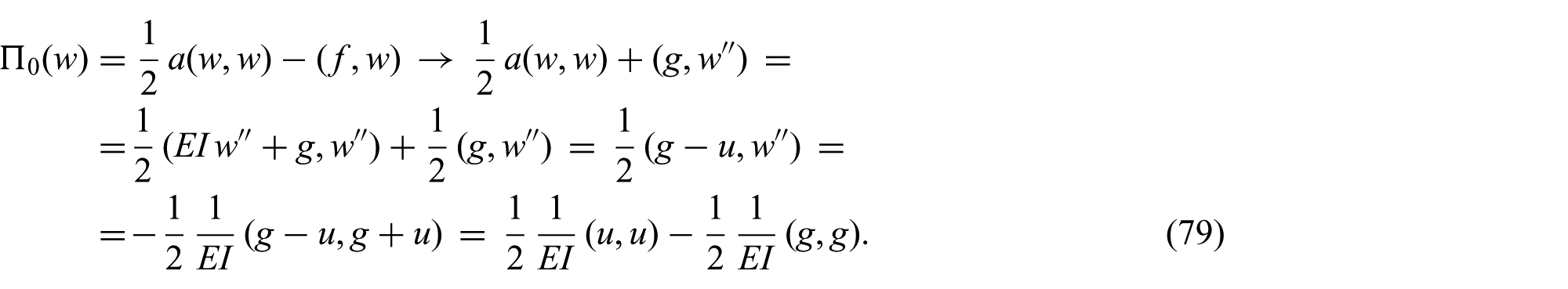
\begin{matrix} Π_{0} (w) = \frac{1}{2} a (w, w) - (f, w) \to \frac{1}{2} a (w, w) + (g, w^{″}) = \\ = \frac{1}{2} (EI w^{″} + g, w^{″}) + \frac{1}{2} (g, w^{″}) = \frac{1}{2} (g - u, w^{″}) = \\ = - \frac{1}{2} \frac{1}{EI} (g - u, g + u) = \frac{1}{2} \frac{1}{EI} (u, u) - \frac{1}{2} \frac{1}{EI} (g, g) . \end{matrix}

(79)

Using equation (79) we are able to finish the conversion of equation (23). We have

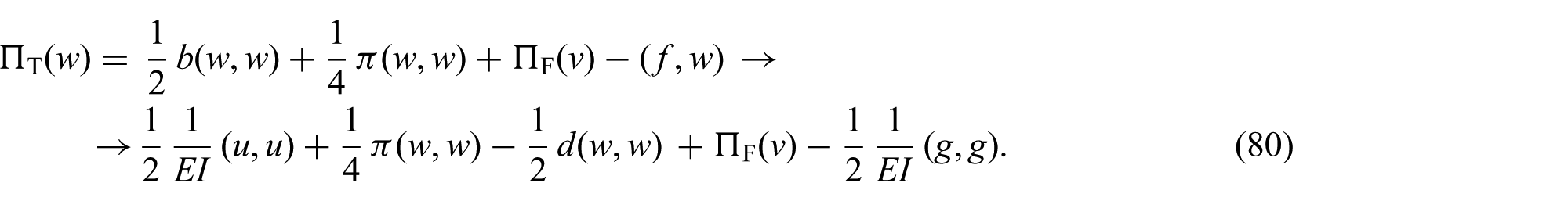
\begin{matrix} Π_{T} (w) = \frac{1}{2} b (w, w) + \frac{1}{4} π (w, w) + Π_{F} (v) - (f, w) \to \\ \to \frac{1}{2} \frac{1}{EI} (u, u) + \frac{1}{4} π (w, w) - \frac{1}{2} d (w, w) + Π_{F} (v) - \frac{1}{2} \frac{1}{EI} (g, g) . \end{matrix}

(80)

The last term in equation (80) is constant, hence it can be omitted by the minimization. Consequently the resulting form is as follows

\begin{matrix} J_{2} (w, u) = \frac{1}{2} \int_{0}^{L} \frac{1}{EI} u^{2} dx + \frac{1}{12} \int_{0}^{L} Eα {(w^{'})}^{4} dx - \frac{1}{2} \int_{0}^{L} Pμ {(w^{'})}^{2} dx + \\ + \frac{1}{2} \int_{0}^{L} c_{F} {({(g - w)}^{+})}^{2} dx . \end{matrix}

(81)

4.4. Solution by means of transformation T2

Now we are ready to realize the original idea of solution from Sofonea and Tiba [8] and Barboteu et al. [9] with a generalization to the Gao beam. But we must be careful, because of satisfying the boundary conditions. Reduction of the state problem to the second-order equation does not enable us to determine arbitrary essential boundary conditions. No more than one in every end-point can be now prescribed.

This is very important from the computational point of view. We are going to use linear finite elements for the reduced state equation, but

we can prescribe only one boundary condition at each end-point and this condition cannot be of the second or the third order,

we are not able to realize accurately essential conditions of the type $v^{'} (0) = 0, v^{'} (L) = 0$ , which are now natural and hence can be satisfied only approximately.

Therefore the only meaningful possibility is the boundary problem (P4), where conditions $v (0) = v (L) = 0$ will be satisfied exactly and the hidden conditions $v^{″} (0) = v^{″} (L) = 0$ are guaranteed by the state equation.

Figure 3.

Simply supported beam with foundation.

Under the assumption, that we have guaranteed the existence of function g such that equation (61) or (62) hold, we can choose $V = V_{4}$ and use transformation T2. The admissible set $U_{ad}$ must be complemented here by additional conditions, as from equations (70) and (72) it follows that $u (0) = u (L) = 0$ . This set will be denoted by $U_{ad}^{0}$ . The associated optimal control problem then has the following form

\begin{matrix} \{\begin{matrix} Find u^{*} \in U_{ad}^{0} such that \\ J_{2} (w (u^{*}), u^{*}) = min_{u \in U_{ad}^{0}} J_{2} (w (u), u), \\ where w : = w (u) \in V_{4} solves the state problem \\ e (w, v) = (g + u, v) \forall v \in V_{4}, \\ with g \in L^{2} ((0, L)) : (g, v^{″}) = - (f, v) \forall v \in V_{4} . \end{matrix} \end{matrix}

(82)

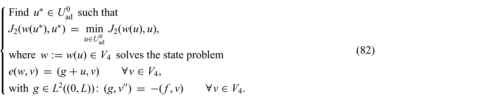
Similarly to section 4.2, we want to establish when the problem (82) has a solution and its relationship to the contact problem (24) or (25) with $V = V_{4}$ .

Theorem 3. Problem (82) has under the assumption $P < P_{cr}^{E}$ exactly one solution.

Proof: is similar to the one of Theorem 1. $□$

Theorem 4. Let there exist a function $g \in L^{2} ((0, L))$ satisfying

\int_{0}^{L} g v^{″} dx = - \int_{0}^{L} fv dx \forall v \in V_{4}

(83)

and let $u^{*}$ solve equation (82). Then the function $w^{*} : = w (u^{*})$ solves the corresponding variational problem (24) on V₄ under the assumption that constant C in $U_{ad}^{0}$ is sufficiently large.

Proof: The ideas involved in the proof of this theorem are quite similar to those involved in the proof of Theorem 2, and, for this reason, it is left. $□$

In conclusion, we will specify optimality conditions regarding the problem (82). Using general results from the Appendix it can be claimed that the pair $(w^{*}, u^{*}) \in V_{4} \times U_{ad}^{0}$ must fulfill

\begin{matrix} e (w^{*}, v) = (g + u^{*}, v) \forall v \in V_{4}, \end{matrix}

(84)

\begin{matrix} e (p^{*}, v) = π (w^{*}, v) - d (w^{*}, v) - κ (w^{*}, v) \forall v \in V_{4}, \end{matrix}

(85)

\begin{matrix} (u^{*} + EI p^{*}, u - u^{*}) & \geq & 0 \forall u \in U_{ad}^{0} . \end{matrix}

(86)

Function $p^{*} \in V_{4}$ represents here the adjoint state and solves the adjoint problem (85). From the other side equation (84) is the state problem referred to in equation (82).

5. Numerical realization and examples

Both the optimal control problems (43) and (82) suggest that a general form of the computational procedure will consist of two parts:

evaluation of the given state problem,

simultaneous minimization of the corresponding functional.

The first item does not make much trouble. The state equation in equation (43) is the Euler–Bernoulli beam equation and its finite element solution is well known and can be found in many books, such as Reddy [15]. As was presented in Machalová and Netuka [11], the matrix form of the state equation can be expressed as

K w = f + B u,

(87)

where $K$ is the well-known stiffness matrix, $f$ is the load vector, $u$ is the vector of control values at nodal points of the finite element mesh and $w$ is the vector of unknown deflections at nodal points. The matrix $B$ represents transition between bases belonging to $w$ and $u$ , hence it is the identity if the two basis are identical. The state equation from equation (82) has formally the same matrix form.

Next, given a control value $u^{n}$ and a computed state $w^{n}$ , we need to perform one step of the minimization process for the corresponding functional $J (w, u)$ . For this purpose we used the conditioned gradient method (see Tröltzsch [19]), where the next iteration $u^{n + 1}$ is found by determining a direction of descent and a suitable step size.

Descent direction means an element $v^{n}$ such that J, in some local neighborhood of $u^{n}$ , is decreasing in the direction $v^{n} - u^{n}$ . Once such a direction is found, one still needs to determine a step size $γ_{n} > 0$ such that $u^{n + 1} = u^{n} + γ_{n} (v^{n} - u^{n})$ is a suitable, i.e. $u^{n + 1} \in U_{ad}$ .

The descent directions were chosen as anti-gradients of $J (w, u)$ , which were evaluated by means of the adjoint problem technique (see Appendix). The adjoint equations (58) and (85) can be solved numerically in a similar way as the state equations.

Step lengths were determined by using standard algorithms, as described in Nocedal and Wright [20].

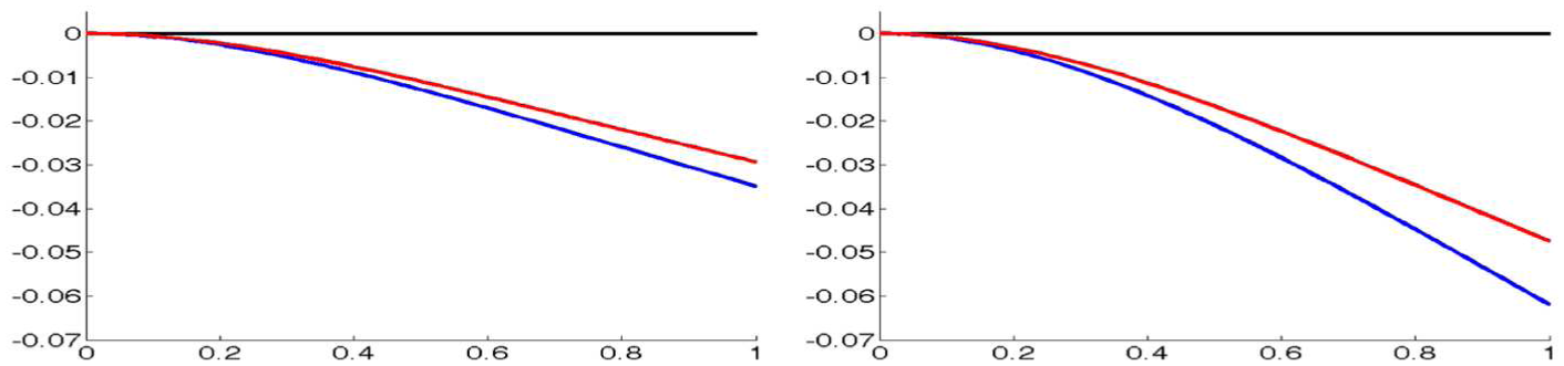
For illustrative purposes, several simple examples are given here. The common data for the beams are: $L = 1 m$ , $h = 0.1 m$ , $E = 21 \cdot 1 0^{10} Pa$ , $I = 0.666 667 \cdot 1 0^{- 3} m^{4}$ , $ν = 0.3$ .

In addition to the Gao beam we will also present results for the classical Euler–Bernoulli beam for comparison. As the nonlinear beam model is in all cases here tougher than the classical one, the upper curves in the following figures show the results for the Gao beam and the lower curves are the results for the Euler–Bernoulli beam.

In the first example pure bending problems are demonstrated for the cantilever beam (see Figure 1) with constant vertical loading $q = - 5 \cdot 1 0^{7} {Nm}^{- 1}$ and different axial forces causing tension (on the left) or compression (on the right), foundation stiffness is in both cases set to zero. Solutions were obtained by means of equation (43), see Figure 4.

Figure 4.

Bending problem (P3) with P = −1 $\cdot 10^{8}$ N (left), $P = + 1 \cdot 10^{8} N$ (right).

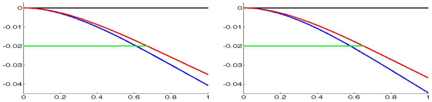
Next we consider contact problems for the cantilever beam (see Figure 1) with constant vertical loading $q = - 5 \cdot 1 0^{7} {Nm}^{- 1}$ and without axial force, the gap is $g = 0.02 m$ . Solutions were obtained by means of equation (43), see Figure 5.

Figure 5.

Problem (P3) with $k_{F} = 5 \cdot 10^{8} {Nm}^{- 2}$ (left) and $k_{F} = 5 \cdot 10^{6} {Nm}^{- 2}$ (right).

The third example is concerned with the propped cantilever beam (see Figure 2) with constant vertical loading $q = - 5 \cdot 1 0^{8} {Nm}^{- 1}$ and different axial forces causing tension (on the left) or compression (on the right), foundation stiffness is in both cases $k_{F} = 5 \cdot 1 0^{8} {Nm}^{- 2}$ , and the gap is $g = 0.007 m$ . Solutions were obtained by means of equation (43), see Figure 6.

Figure 6.

Problem (P2) with $P = - 5 \cdot 10^{9} N$ (left) and $P = + 10^{8} N$ (right).

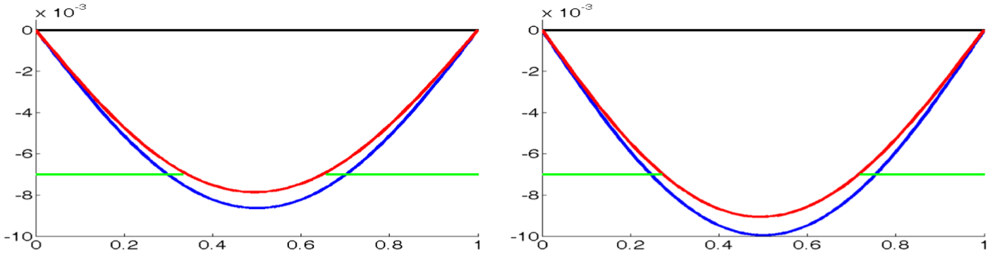
The last example is related to the simply supported beam (see Figure 3) with constant vertical loading $q = - 1 \cdot 1 0^{8} {Nm}^{- 1}$ and different axial forces causing tension (on the left) or compression (on the right), foundation stiffness is in both cases $k_{F} = 5 \cdot 1 0^{8} {Nm}^{- 2}$ , and the gap is $g = 0.007 m$ . Solutions were obtained by means of equation (82), see Figure 7.

Figure 7.

Problem (P4) with $P = - 1 \cdot 10^{8} N$ (left) and $P = + 1 \cdot 10^{8} N$ (right).

Remark: From numerical experiments it was established that 32 finite elements lasts for sufficiently accurate computations.

6. Conclusion

In the papers by Sofonea and Tiba [8] and Barboteu et al. [9] the control variational method was applied to contact of a vertically loaded linear cantilever beam and an elastic foundation. Our research considerably generalizes these works as we consider a nonlinear beam, which is in addition also subjected to axial load and all standard boundary conditions can be applied. We also expanded and refined a numerical solution for this approach. Our examples show that the method works well. Furthermore, for the reduced state equation it goes evidently faster.

There is a natural direction for future research: extension of considered problems to nonconvex cases. The authors believe that the control variational method will be useful also for this purpose.

Footnotes

Appendix: Optimal control problem

Here we want to present a brief overview of basic concepts and results regarding the optimal control of problems governed by elliptic differential equations. They consist of the so-called state problem containing control parameter and optimization of certain functionals with respect to this control parameter. Especially we will deal with control by the right-hand side of the state equation, see Lions [21] and Tröltzsch [19].

Definition 1.Let V be a Hilbert space, $V^{'}$ its dual, $a : V \times V \to ℝ$ be a bounded V -elliptic bilinear form. Let U be a reflexive Banach space, $U_{ad}$ be a nonempty subset of U, $B : U \to V^{'}$ a linear continuous mapping, i.e. $B \in L (U, V^{'})$ . For any $u \in U_{ad}$ we will consider the problem

(88)

\{\begin{matrix} Find w : = w (u) \in V such that \\ a (w, v) = {⟨ f + Bu, v ⟩}_{V^{'} \times V} \forall v \in V, \end{matrix}

where $f \in V^{'}$ is a given element and ${⟨ ., . ⟩}_{V^{'} \times V}$ denotes the duality pairing between $V^{'}$ and V.

Problem (88) will be called the variational formulation of the state problem and w will be the state of the system described by equation (88). Moreover, U will be the space of controls and $U_{ad}$ the set of admissible controls.

The state problem can also be formulated as a differential equation. But variational formulation (88) is more suitable especially if we want to use the FEM for its numerical solution.

Next we introduce the so-called cost or objective functional $J : V \times U \to ℝ$ , which serves to obtain a suitable solution of the given state problem (88).

Definition 2. Let V be a Hilbert space, $U_{ad}$ be a nonempty subset of Banach space U and $J : V \times U \to ℝ$ be the given cost functional.

The problem

(89)

\{\begin{matrix} Find u^{*} \in U_{ad} such that \\ J (w (u^{*}), u^{*}) = \min_{u \in U_{ad}} J (w (u), u), \\ where w (u) \in V solves the state problem (88), \end{matrix}

is called the optimal control problem for the elliptic state equation (88) by the right-hand side.

Of course, we need to know the conditions that can guarantee the existence of a solution for the problem (89).

Theorem 5. Let V be a Hilbert space, $U_{ad} \neq \emptyset$ be a bounded closed convex subset of a reflexive Banach space U and $J : V \times U \to ℝ$ be a given functional.

If J is weakly lower semicontinuous on $V \times U$ , i.e.

(90)

w_{n} ⇀ w, u_{n} ⇀ u \Rightarrow \underset{n \to + \infty}{liminf} J (w_{n}, u_{n}) \geq J (w, u),

then the optimal control problem (89) has at least one solution.

Proof can be found in Lions [21] or Machalová and Netuka [11].

Taking into account Theorem 5, we will always suppose that $U_{ad}$ is a nonempty bounded closed convex subset of U.

Generally it is very useful to determine optimality conditions for our problem (89). If we introduce a linear operator $A \in L (V, V^{'})$ by the relation

(91)

{⟨ Aw, v ⟩}_{V^{'} \times V} = a (w, v) \forall w, v \in V,

they can be established by means of the Lagrange multiplier technique as follows (see Machalová and Netuka [11])

(92)

\begin{matrix} {⟨ \nabla_{w} J (w, u), w ⟩}_{V^{'} \times V} - {⟨ Aw, p ⟩}_{V^{'} \times V} = 0 \forall w \in V, \end{matrix}

(93)

\begin{matrix} {⟨ \nabla_{u} J (w, u), z - u ⟩}_{U^{'} \times U} + {⟨ B^{*} p, z - u ⟩}_{U^{'} \times U} & \geq & 0 \forall z \in U_{ad}, \end{matrix}

(94)

\begin{matrix} {⟨ f + Bu, p ⟩}_{V^{'} \times V} - {⟨ Aw, p ⟩}_{V^{'} \times V} = 0 \forall p \in V, \end{matrix}

where $B^{*} \in L (V, U^{'})$ is the adjoint operator to B, i.e. it fulfills

(95)

{⟨ z, B^{*} p ⟩}_{U \times U^{'}} = {⟨ Bz, p ⟩}_{V^{'} \times V} \forall z \in U, p \in V .

Introducing analogously the adjoint operator $A^{*}$ by

(96)

{⟨ A^{*} w, v ⟩}_{V^{'} \times V} = a^{*} (w, v) = a (v, w) \forall w, v \in V,

the expressions (92)–(94) can be rewritten as follows

(97)

\begin{matrix} a^{*} (p, v) = {⟨ \nabla_{w} J (w, u), v ⟩}_{V^{'} \times V} \forall v \in V, \end{matrix}

(98)

\begin{matrix} {⟨ \nabla_{u} J (w, u) + B^{*} p, z - u ⟩}_{U^{'} \times U} & \geq & 0 \forall z \in U_{ad}, \end{matrix}

(99)

\begin{matrix} a (w, p) = {⟨ f + Bu, p ⟩}_{V^{'} \times V} \forall p \in V . \end{matrix}

Moreover, from equation (99) the operator form of the state equation

(100)

Aw = f + Bu in V^{'}

and from equation (97) the so-called adjoint equation

(101)

A^{*} p = \nabla_{w} J (w, u) in V^{'}

can be deduced.

Finally, we will study the dependence of the functional $J (w (u), u)$ on u. For this purpose let us rewrite the state problem (88) as the operator equation

(102)

Aw (u) = f + Bu .

From here we get

(103)

w (u) = A^{- 1} Bu + A^{- 1} f,

i.e. the mapping $Φ : u \mapsto w (u)$ is affine and therefore its Frechet derivative is done by

(104)

w^{'} (u, φ) = Φ^{'} (u) φ = A^{- 1} B φ \forall φ \in V .

This implies that $w^{'} (u, φ) \in V$ solves

(105)

a (w^{'} (u, φ), v) = {⟨ B φ, v ⟩}_{V^{'} \times V} \forall v \in V .

Now we denote

(106)

I (u) \equiv J (w (u), u) \forall u \in U_{ad}

and let us analyze the properties of the mapping $u \mapsto I (u)$ .

Let J be differentiable on $V \times U$ and at a point $(w, u)$ there exists the gradient $\nabla_{w} J (w, u) \in V^{'}$ with respect to w and the gradient $\nabla_{u} J (w, u) \in U^{'}$ with respect to u. Then I is also differentiable on U and has the gradient $\nabla_{u} I (u) \in U^{'}$ at u. From the chain rule we can deduce

(107)

{⟨ \nabla_{u} I (u), z ⟩}_{U^{'} \times U} = {⟨ \nabla_{w} J (w, u), w^{'} (u, z) ⟩}_{V^{'} \times V} + {⟨ \nabla_{u} J (w, u), z ⟩}_{U^{'} \times U} \forall z \in U .

Here we are able to rewrite the first term on the right-hand side. Let $p = p (u) \in V$ be a solution of the adjoint equation (97), where the bilinear form $a^{*}$ is defined by equation (96). Substituting $w^{'} (u, z)$ for v into equation (97) we get

(108)

a^{*} (p, w^{'} (u, z)) = {⟨ \nabla_{w} J (w, u), w^{'} (u, z) ⟩}_{V^{'} \times V} .

Using this expression we obtain according to equations (96), (105) and (95) from equation (107) finally

(109)

{⟨ \nabla_{u} I (u), z ⟩}_{U^{'} \times U} = {⟨ B^{*} p, z ⟩}_{U^{'} \times U} + {⟨ \nabla_{u} J (w, u), z ⟩}_{U^{'} \times U} \forall z \in U

(110)

\nabla_{u} I (u) = B^{*} p + \nabla_{u} J (w, u) .

Hence, by means of the adjoint state method we are able to evaluate the gradient of I(u).

Funding

This research received no specific grant from any funding agency in the public, commercial, or not-for-profit sectors.

References

Sofonea

Matei

. Mathematical models in contact mechanics. Cambridge: Cambridge University Press, 2012.

Gao

Machalová

Netuka

. Mixed finite element solutions to contact problems of nonlinear Gao beam on elastic foundation. Nonlinear Anal Real World Appl 2015; 22: 537–550.

Shillor

Sofonea

Telega

. Models and analysis of quasistatic contact: Variational methods. Berlin: Springer-Verlag, 2004.

Arnautu

Langmach

Sprekels

Tiba

. On the approximation and the optimization of plates. Numer Funct Anal Optim 2000; 21: 337–354.

Sprekels

Tiba

. Control variational methods for differential equations. In: Hoffmann

K-H

et al . (eds.) Optimal control of complex structures. Basel: Birkhäuser, 2001, 245–257.

Sofonea

Tiba

. The control variational method for elastic contact problems. Ann Acad Rom Sci Ser Math Appl 2010; 2: 99–122.

Tiba

. Optimal control methods and the variational approach to differential equations. In: Ao

et al . (eds.) Lecture notes in engineering and computer science: Proceedings of IMECS 2013. Hong Kong: Newswood, 2013, 127–132.

Sofonea

Tiba

. The control variational method for contact of Euler–Bernoulli beams. Bull Transilvania Univ Brasov, Ser III 2009: 2: 127–136.

Barboteu

Sofonea

Tiba

. The control variational method for beams in contact with deformable obstacles. Z Angew Math Mech 2012; 92: 25–40.

10.

Neittaanmäki

Sprekels

Tiba

. Optimization of elliptic systems. Theory and applications. New York: Springer, 2006.

11.

Machalová

Netuka

. Solution of contact problems for nonlinear Gao beam and obstacle. J Appl Math 2015; 2015: 420649.

12.

Andrews

Dumont

M’Bengue

et al . Analysis and simulations of a nonlinear dynamic beam. J Appl Math Phys 2012; 63: 1005–1019.

13.

Andrews

Kuttler

Shillor

. Dynamic Gao beam in contact with a reactive or rigid foundation. In: Han

et al . (eds.) Advances in variational and hemivariational inequalities with applications (Advances in Mechanics and Mathematics, vol. 33). Cham: Springer, 2015, 225–248.

14.

Ahn

Kuttler

Shillor

. Dynamic contact of two Gao beams. Electron J Diff Eqn 2012; 2012: 1–42.

15.

Reddy

. An introduction to the finite element method. New York: McGraw-Hill, 2006.

16.

Gao

. Nonlinear elastic beam theory with application in contact problems and variational approaches. Mech Res Commun 1996; 23: 11–17.

17.

Gao

Ogden

. Closed-form solutions, extremality and nonsmoothness criteria in a large deformation elasticity problem. Z Angew Math Mech 2008; 59: 498–517.

18.

Kravchuk

Neittaanmäki

. Variational and quasi-variational inequalities in mechanics (Solid Mechanics and its Applications, book 147). New York: Springer, 2007.

19.

Tröltzsch

. Optimal control of partial differential equations. Theory, methods and applications. Providence: AMS, 2010.

20.

Nocedal

Wright

. Numerical optimization. New York: Springer-Verlag, 2006.

21.

Lions

. Optimal control of systems governed by partial differential equations. Berlin: Springer-Verlag, 1971.