Brachistochronic motion of a nonholonomic variable-mass mechanical system in general force fields

Abstract

In this paper, the brachistochronic motion of a mechanical system composed of variable-mass particles is analysed. Workless (ideal) holonomic and linear nonholonomic constraints are imposed on the system. It is assumed that the system moves in an arbitrary field of known potential and nonpotential forces with prescribed both laws of the time-rate of mass variation of the particles and relative velocities of the expelled (or gained) masses. The first time-derivatives of quasi-velocities are taken as control variables. Using Pontryagin’s maximum principle and singular optimal control theory, the problem of brachistochronic motion of the nonholonomic variable-mass mechanical system is solved as a two-point boundary value problem. In addition, a discussion about the realization of control forces is given. The results are illustrated via an example.

Keywords

Brachistochrone variable mass nonholonomic constraints Chaplygin sleigh singular controls

1. Introduction

The literature treating nonholonomic variable-mass mechanical systems is rather scarce. The considered class of mechanical systems can embrace important engineering systems such as underwater vehicles, ground mobile robots and manipulators, excavating machines, etc. The available field-related literature can be separated into two groups. The first group includes [1 –5], whereas the second covers [6 –8]. Note that detailed literature overviews related to holonomic variable-mass mechanical systems is given in [9 –12]. The authors in [1 –5] consider various problems of analytical mechanics related to nonholonomic variable-mass mechanical systems. Thus, [1 –3] discuss the application of Kane’s equations, D’Alembert–Lagrange’s principle and Gibbs–Appell’s equations, respectively, in the case of nonholonomic variable-mass systems, while in [4] the extension of Hamilton’s principle application to this kind of mechanical system is given. On the other hand, in [5], Routh’s equations were derived for a variable-mass mechanical system with nonlinear nonholonomic constraints moving in a noninertial reference frame. The problem of control of variable-mass mechanical systems with nonholonomic constraints is addressed in [6 –8]. Note that in [8] the problem of the brachistochronic motion of a nonholonomic two-degree-of-freedom (2DOF) system composed of two variable-mass particles is considered. For the case of the brachistochronic motion of variable-mass mechanical systems with holonomic constraints, see [9].

The goal of our paper is to generalize the results from [8] in the case of an arbitrary variable-mass mechanical system with linear nonholonomic constraints with arbitrary degrees of freedom that performs the brachistochronic motion in an arbitrary field of known potential and nonpotential forces. To the best of our knowledge, this kind of problem has not been reported elsewhere before. In this respect, the paper is organized as follows: in Section 2 the brachistochrone problem of a variable-mass mechanical system with linear nonholonomic constraints is formulated. In Section 3 using the first time-derivatives of quasi-velocities as control variables, the brachistochrone problem is formulated as a singular optimal control task. The corresponding two-point boundary value problem (TPBVP) is defined and the numerical procedure for solving it based on the shooting method is described. The discussion about the realization of brachistochronic motion is shown in Section 4. In Section 5, in order to illustrate the application of the obtained theoretical results, a modified example from [8] is considered. Conclusions are presented in Section 6.

2. Problem formulation

Consider the motion of a mechanical system composed of N particles that can all be of variable mass in a general case. The configuration of the system is defined by $n$ generalized coordinates $q = (q^{1}, q^{2}, \dots, q^{n})^{T}$ , which determine the position of the system but are geometrically independent. Also, the laws of mass variation of the particles are well-known

m_{p} = m_{p} (t), p = 1, \dots, N,

(1)

where $m_{p} (t)$ are continuous and differentiable functions of time. Mass variation of the particles may occur due to expelled (or gained) masses of the particles, assuming that the process of expelling (or gaining) is continuous over the observed interval of time.

Relative velocities of expelled (or gained) masses are

{\vec{v}}_{p}^{rel} = {\vec{v}}_{p}^{rel} (q, \overset{\cdot}{q}, t), p = 1, \dots, N,

(2)

where $\overset{\cdot}{q} = ({\overset{\cdot}{q}}^{1}, {\overset{\cdot}{q}}^{2}, \dots, {\overset{\cdot}{q}}^{n})^{T}$ is the vector of generalized velocities. The kinetic energy of a scleronomic mechanical system is a homogeneous quadratic form of the generalized velocities [13 –15]

T = \frac{1}{2} a_{ij} {\overset{\cdot}{q}}^{i} {\overset{\cdot}{q}}^{j}, i, j = 1, \dots, n,

(3)

where covariant coordinates of the metric tensor, taking into account (1), are the functions of the generalized coordinates and time t

a_{ij} = a_{ij} (q, t) .

(4)

Note that in this paper the well-known summation convention over pairs of Latin or Greek indices is used, with the following index ranges: $i, j, k, r = 1, \dots, n;$ $α, β, γ, δ = 1, \dots, m;$ $v, ρ = m + 1, \dots, n;$ $s, z = 1, . . ., m - 1$ . The motion of the considered mechanical system is constrained by $l$ ideal independent nonholonomic homogeneous mechanical constraints of the form

ψ^{v} (q, \overset{\cdot}{q}) \equiv {\overset{\cdot}{q}}^{v} - b_{α}^{v} {\overset{\cdot}{q}}^{α} = 0,

(5)

where $b_{α}^{v} = b_{α}^{v} (q)$ . The number of degrees of freedom of the mechanical system is m = n – l, which simultaneously represents the number of kinematically independent coordinates $q^{α}$ that correspond to independent generalized velocities ${\overset{\cdot}{q}}^{α}$ .

Independent generalized velocities can be represented as a linear form of independent quasi-velocities ${\overset{\cdot}{π}}^{1}, . . ., {\overset{\cdot}{π}}^{m}$ [13 –15]

{\overset{\cdot}{q}}^{α} = c_{β}^{α} {\overset{\cdot}{π}}^{β} .

(6)

Dependent generalized velocities, taking into account (5) and (6), can be expressed as follows

{\overset{\cdot}{q}}^{v} = c_{β}^{ν} {\overset{\cdot}{π}}^{β},

(7)

where $c_{β}^{ν} = b_{α}^{v} c_{β}^{α}$ , and therefore the expressions for transformation of all generalized velocities, in accordance with (6) and (7), can be expressed as a linear form of independent quasi-velocities

{\overset{\cdot}{q}}^{i} = c_{α}^{i} {\overset{\cdot}{π}}^{α},

(8)

where $c_{α}^{i} = c_{α}^{i} (q)$ are continuous functions with continuous first derivatives in the region in which the motion of a mechanical system is considered. Thus, the kinetic energy of a nonholonomic scleronomic mechanical system, in accordance with (3) and (8), can be expressed as a homogeneous quadratic form of independent quasi-velocities

T^{*} = \frac{1}{2} G_{α β} {\overset{\cdot}{π}}^{α} {\overset{\cdot}{π}}^{β},

(9)

where

G_{α β} (q, t) = a_{ij} c_{α}^{i} c_{β}^{j},

(10)

and where $G_{α β}$ are covariant coordinates of the metric tensor. Let the mechanical system move in the field of known potential forces with potential energy

Π = Π (q, t),

(11)

and let the system be acted on by arbitrary known nonpotential forces, whose generalized forces are of the form

Q_{i}^{w} = Q_{i}^{w} (q, \overset{\cdot}{q}, t) .

(12)

In order to derive differential equations that describe the motion of a nonholonomic mechanical system in the configuration space of kinematically independent coordinates, let us commence from the expression for the Lagrange–D’Alembert principle [13 –15] written in the form

a_{ij} (a^{j} - Q^{j}) δ q^{i} = 0,

(13)

that is

(a_{ij} a^{j} - Q_{i}) δ q^{i} = 0,

(14)

where $Q_{i}$ are the covariant generalized forces corresponding to the geometrically independent coordinates.

The contravariant coordinates of acceleration [13 –15] can be expressed in the following way

a^{j} = {\overset{\cdot\cdot}{q}}^{j} + Γ_{kr}^{j} {\overset{\cdot}{q}}^{k} {\overset{\cdot}{q}}^{r},

(15)

where $Γ_{kr}^{j}$ are the Christoffel symbols of the second kind.

In accordance with the Hertz–Hölder condition [16,17], based on (8), we may write

δ q^{i} = c_{α}^{i} δ π^{α} .

(16)

Taking into account (8), (14), (15) and (16), and after a brief rearrangement, the following is obtained

(a_{ij} c_{β}^{j} {\overset{\cdot\cdot}{π}}^{β} + a_{ij} \frac{\partial c_{β}^{j}}{\partial q^{k}} c_{γ}^{k} {\overset{\cdot}{π}}^{γ} {\overset{\cdot}{π}}^{β} + a_{ij} Γ_{kr}^{j} c_{γ}^{k} c_{β}^{r} {\overset{\cdot}{π}}^{γ} {\overset{\cdot}{π}}^{β} - Q_{i}) c_{α}^{i} δ π^{α} = 0 .

(17)

From expression (17), due to independence of variations $δ π^{α}$ , that is, $δ π^{α} \neq 0$ , m differential equations are obtained in the covariant form

G_{α β} {\overset{\cdot\cdot}{π}}^{β} + a_{ij} c_{α}^{i} c_{γ}^{k} (\frac{\partial c_{β}^{j}}{\partial q^{k}} + Γ_{kr}^{j} c_{β}^{r}) {\overset{\cdot}{π}}^{γ} {\overset{\cdot}{π}}^{β} = {\tilde{Q}}_{α},

(18)

where generalized forces corresponding to the kinematically independent coordinates are given as

{\tilde{Q}}_{α} (q, \overset{\cdot}{π}, t) = c_{α}^{i} Q_{i},

(19)

whereas $\overset{\cdot}{π} = ({\overset{\cdot}{π}}^{1}, {\overset{\cdot}{π}}^{2}, \dots, {\overset{\cdot}{π}}^{m})^{T}$ .

Equation (18) can be represented in the form as follows

G_{α β} {\overset{\cdot\cdot}{π}}^{β} = Δ_{α},

(20)

where

Δ_{α} (q, \overset{\cdot}{π}, t) = {\tilde{Q}}_{α} - a_{ij} c_{α}^{i} c_{γ}^{k} (\frac{\partial c_{β}^{j}}{\partial q^{k}} + Γ_{kr}^{j} c_{β}^{r}) {\overset{\cdot}{π}}^{γ} {\overset{\cdot}{π}}^{β} .

(21)

The generalized forces corresponding to the geometrically independent coordinates can be represented, in a general case, in the following form

Q_{i} (q, \overset{\cdot}{q}, t) = - \frac{\partial Π}{\partial q^{i}} + {Q_{i}}^{w} + {Q_{i}}^{var} + {Q_{i}}^{c} + {Q_{i}}^{Λ} .

(22)

The generalized reactive forces that develop due to expelled (or gained) masses are of the form [18,19]

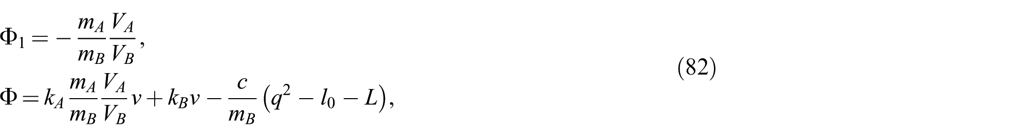
Q_{i}^{var} (q, \overset{\cdot}{q}, t) = \sum_{p = 1}^{N} {\overset{\cdot}{m}}_{p} {\vec{v}}_{p}^{rel} \cdot \frac{\partial {\vec{r}}_{p}}{\partial q^{i}},

(23)

while ${Q_{i}}^{c} = {Q_{i}}^{c} (q, \overset{\cdot}{q}, t)$ - are the generalized control forces, whose total power during brachistochronic motion equals zero

Q_{i}^{c} {\overset{\cdot}{q}}^{i} = 0,

(24)

whereas, in accordance with (8) and (19), the previous expression can be written in the following form

{\tilde{Q}}_{α}^{c} {\overset{\cdot}{π}}^{α} = 0 .

(25)

Note that it is necessary to make a distinction between the brachistochronic motion of the mechanical systems and the time-optimal motion problem of mechanical systems. In both problems the time of motion of a mechanical system is minimized. However, in solving the brachistochrone problem the condition that the power of control forces equals zero is imposed. For example, in the case of Bernoulli’s brachistochrone the control force represents the reaction of a frictionless cycloid. More details about the choice of control forces for realization of the brachistochronic motion of mechanical systems can be found in [20]. On the other hand, an example of technical facility where the time-optimal motion problem is considered (the power of control forces does not equal zero) can be a robotic mechanism where the operation of robot gripper displacement from the specified initial to specified terminal position in a minimum time is realized by control forces representing driving forces in joints of the robot (see e.g. [21]).

Since generalized forces, due to imposed constraints of motion (5), can be represented in the form as follows

Q_{i}^{Λ} (q, \overset{\cdot}{q}) = Λ_{v} \frac{\partial ψ^{v}}{\partial {\overset{\cdot}{q}}^{i}},

(26)

where $Λ_{v}$ are Lagrange’s multipliers of constraints, and based on (5), (19) and (26), we can write

{\tilde{Q}}_{α}^{Λ} = c_{α}^{β} Q_{β}^{Λ} + c_{α}^{ν} Q_{v}^{Λ} = Λ_{v} (c_{α}^{v} - c_{α}^{β} b_{β}^{v}) .

(27)

Since according to (7)

c_{α}^{v} = c_{α}^{β} b_{β}^{v},

(28)

the generalized forces ${\tilde{Q}}_{α}^{Π}$ become

{\tilde{Q}}_{α}^{Λ} = 0 .

(29)

Thus, it has been shown that unknown Lagrange’s multipliers of constraints $Λ_{v}$ do not figure in the differential equations of motion (20), that is, in the configuration space of kinematically independent coordinates, whereby the procedure for determining the system motion relative to the procedure for determining the reactions of nonholonomic constraints is completely separated. Multiplying both sides of equation (20) by ${\overset{\cdot}{π}}^{α}$ and summing over an index $α$ the following is obtained

G_{α β} {\overset{\cdot\cdot}{π}}^{β} {\overset{\cdot}{π}}^{α} = Δ_{α} {\overset{\cdot}{π}}^{α},

(30)

which can be written in the following form

G_{α s} {\overset{\cdot\cdot}{π}}^{α} {\overset{\cdot}{π}}^{s} + G_{α m} {\overset{\cdot\cdot}{π}}^{m} {\overset{\cdot}{π}}^{α} = Δ_{α} {\overset{\cdot}{π}}^{α} .

(31)

The last relation enables one to express one arbitrary second time-derivative of a quasi-coordinate as a function of the rest. Taking into account (25) and (29), in equation (31) unknown multipliers of constraints will not figure, nor will the generalized control forces. Now, without loss of generality, we are able to express ${\overset{\cdot\cdot}{π}}^{m}$ from relation (31) in the following form

{\overset{\cdot\cdot}{π}}^{m} = Φ + Φ_{s} {\overset{\cdot\cdot}{π}}^{s},

(32)

where

Φ (q, \dot{π}, t) = \frac{Δ_{β} {\dot{π}}^{β}}{G_{α m} {\dot{π}}^{α}}, Φ_{s} (q, \dot{π}, t) = - \frac{G_{β s} {\dot{π}}^{β}}{G_{α m} {\dot{π}}^{α}},

(33)

where it is assumed that the expression $G_{α m} {\overset{\cdot}{π}}^{α}$ that figures in the denominators of the relations (33) does not equal zero during the system motion, that is, $G_{α m} {\overset{\cdot}{π}}^{α} \neq 0 \forall t \in [t_{0}, t_{f}]$ , where $t_{0}$ and $t_{f}$ are the initial and final time moment corresponding to the initial and final system position, respectively.

Let the values of generalized coordinates and the value of the system mechanical energy be specified at the initial time moment of motion

t_{0} = 0, q (t_{0}) = q_{0},

(34)

T^{*} (q_{0}, {\overset{\cdot}{π}}_{0}, t_{0}) + Π (q_{0}, t_{0}) = E_{0},

(35)

and also the values of generalized coordinates at the final system position

q (t_{f}) = q_{f},

(36)

where $E_{0} \in R$ and $t_{f} \in R$ . The problem of brachistochronic motion of a nonholonomic variable-mass mechanical system in the arbitrary force fields, whose differential equations of motion are given in the form (20), consists of defining the control forces $Q_{i}^{c} = Q_{i}^{c} (t)$ as well as their corresponding system motions $q^{i} (t)$ , so that the system moves in a minimum time $t_{f}$ from the known initial state described by (34) and (35) to the final specified state described by (36).

3. The brachistochrone problem as an optimal control task

The presented brachistochrone problem can be formulated as a task of optimal control by introducing the controls $u^{s}$

u^{s} = {\overset{\cdot\cdot}{π}}^{s} .

(37)

Without loss of generality, the renaming of the variable of the form $V^{α} = {\overset{\cdot}{π}}^{α}$ is introduced, and therefore

V = (V^{1}, V^{2}, \dots, V^{m})^{T} .

(38)

First-order differential equations in the normal form, which are known in the optimal control theory as state equations, can be written by introducing the rheonomic coordinate $q^{n + 1} \overset{Δ}{=} t$ as follows

\begin{matrix} {\overset{\cdot}{q}}^{i} = f_{i} (q, V, q^{n + 1}, u) \equiv c_{β}^{i} V^{β}, \\ {\overset{\cdot}{q}}^{n + 1} = f_{n + 1} (q, V, q^{n + 1}, u) \equiv 1, \\ {\overset{\cdot}{V}}^{s} = f_{n + 1 + s} (q, V, q^{n + 1}, u) \equiv u^{s}, \\ {\overset{\cdot}{V}}^{m} = f_{n + 1 + m} (q, V, q^{n + 1}, u) \equiv Φ (q, V, q^{n + 1}) + Φ_{s} (q, V, q^{n + 1}) u^{s}, \end{matrix}

(39)

where $u = (u^{1}, u^{2}, \dots, u^{m - 1})^{T}$ as well as $u^{s} (\cdot) : [0, t_{f}] \to R$ .

The problem of the brachistochronic motion of the considered nonholonomic mechanical system described by the state equations (39) consists of determining the optimal controls $u^{s}$ , as well as their corresponding optimal trajectories in the state space $q^{i} (t)$ , so that the system moves from the known initial state on the manifold (34) to the final specified state on the manifold (36), with a defined value of the system mechanical energy at the initial time moment (35), in a minimum time. It can be expressed in the form of the condition that the functional

J (q, V, q^{n + 1}, u) = \int_{0}^{t_{f}} dt,

(40)

over the interval $[0, t_{f}]$ has a minimum value. In order to solve the optimum control task, formulated by the Pontryagin maximum principle [22], the Hamiltonian [22] is formed as follows

H (q, V, q^{n + 1}, u, λ, ν) = - 1 + λ_{j} c_{β}^{j} V^{β} + λ_{n + 1} + ν_{s} u^{s} + ν_{m} (Φ + Φ_{s} u^{s}),

(41)

where $λ = {(λ_{1}, λ_{2}, . . ., λ_{n + 1})}^{T}$ , $ν = {(ν_{1}, ν_{2}, . . ., ν_{m})}^{T}$ , whereas $λ_{i} (\cdot) : [0, t_{f}] \to R, λ_{n + 1} (\cdot) : [0, t_{f}] \to R$ and $ν_{α} (\cdot) : [0, t_{f}] \to R$ are costate variables, so that the costate system of differential equations is of the form

\begin{matrix} {\overset{\cdot}{λ}}_{i} = - \frac{\partial H}{\partial q^{i}} = - λ_{j} \frac{\partial c_{β}^{j}}{\partial q^{i}} V^{β} - ν_{m} (\frac{\partial Φ}{\partial q^{i}} + \frac{\partial Φ_{s}}{\partial q^{i}} u^{s}), \\ {\overset{\cdot}{λ}}_{n + 1} = - \frac{\partial H}{\partial q^{n + 1}} = - λ_{j} \frac{\partial c_{β}^{j}}{\partial q^{n + 1}} V^{β} - ν_{m} (\frac{\partial Φ}{\partial q^{n + 1}} + \frac{\partial Φ_{s}}{\partial q^{n + 1}} u^{s}), \\ {\overset{\cdot}{ν}}_{α} = - \frac{\partial H}{\partial V^{α}} = - λ_{j} c_{α}^{j} - ν_{m} (\frac{\partial Φ}{\partial V^{α}} + \frac{\partial Φ_{s}}{\partial V^{α}} u^{s}) . \end{matrix}

(42)

Based on (41) it can be written

H (q, V, q^{n + 1}, u, λ, ν) = H_{0} + H_{s} u^{s},

(43)

where

\begin{matrix} H_{0} = - 1 + λ_{j} c_{β}^{j} V^{β} + λ_{n + 1} + ν_{m} Φ, \\ H_{s} = ν_{s} + ν_{m} Φ_{s}, \end{matrix}

(44)

and it is where such a case is referred to as singular in the optimal control theory, and therefore the necessary optimality conditions of the Pontryagin maximum principle are of the form

\frac{\partial H}{\partial u^{s}} = H_{s} = 0,

(45)

from where optimal controls $u^{s}$ cannot be explicitly defined. Now, the boundary conditions can be represented in the following form

{(λ_{i} Δ q^{i} + λ_{n + 1} Δ q^{n + 1} + ν_{s} Δ V^{s} + ν_{m} Δ V^{m}) |}_{0}^{t_{f}} = 0,

(46)

{(H Δ t) |}_{0}^{t_{f}} = 0,

(47)

where $Δ (\cdot)$ represents the noncontemporaneous variation [13,15] of the quantity (·).

Based on condition (45), we are able to express the costate variables $ν_{s}$ as the functions of a costate variable $ν_{m}$ in the form

ν_{s} = - ν_{m} Φ_{s} .

(48)

Accordingly, the necessary conditions (45) require that the coefficients $H_{s}$ in (43) be identically equal to zero along the optimal state trajectory. Optimal controls $u^{s}$ are defined by further differentiation with respect to time (45) in accordance with (39) and (42)

\frac{d^{k}}{d t^{k}} [\frac{\partial H}{\partial u^{s}}] = 0, k = 0, 1, 2, . . .

(49)

In determining the relations (49), a well-known Poisson brackets formalism [23] is applied, so that

{\overset{\cdot}{H}}_{s} = {H, H_{s}} = {H_{s}, H_{0}} + {H_{s}, H_{z}} u^{z} = 0 .

(50)

Taking into account (45) as well as the fact that for multidimensional singular controls [23] along an optimal trajectory it holds that

{H_{s}, H_{z}} = 0,

(51)

it is obtained that

{H_{s}, H_{0}} = \sum_{ϑ = 1}^{n + 1 + m} (\frac{\partial H_{s}}{\partial x^{ϑ}} \frac{\partial H_{0}}{\partial ξ^{ϑ}} - \frac{\partial H_{s}}{\partial ξ^{ϑ}} \frac{\partial H_{0}}{\partial x^{ϑ}}) = 0,

(52)

where $x = (x^{1}, x^{2}, \dots, x^{n + 1 + m})^{T} \overset{Δ}{=} (q^{1}, q^{2}, \dots, q^{n + 1}, V^{1}, V^{2}, . . ., V^{m})^{T}$ and $ξ = (ξ^{1}, ξ^{2}, \dots, ξ^{n + 1 + m})^{T} \overset{Δ}{=}$

(λ_{1}, λ_{2}, \dots, λ_{n + 1}, ν_{1}, ν_{2}, . . ., ν_{m})^{T} .

Now, from equations (52), taking into account (44) and (48), the next relations follows

λ_{z} (q, V, q^{n + 1}, λ_{m}, λ_{m + 1}, . . ., λ_{n}, ν_{m}) = Ω_{z}^{s} (ν_{m} φ_{s} - λ_{m} ω_{s}^{m} - λ_{ρ} ω_{s}^{ρ}),

(53)

where

\begin{matrix} φ_{s} = \frac{\partial Φ_{s}}{\partial q^{i}} c_{α}^{i} V^{α} + \frac{\partial Φ_{s}}{\partial q^{n + 1}} + \frac{\partial Φ_{s}}{\partial V^{m}} Φ - \frac{\partial Φ}{\partial V^{s}} - \frac{\partial Φ}{\partial V^{m}} Φ_{s}, \\ ω_{s}^{m} = c_{s}^{m} + c_{m}^{m} Φ_{s}, \\ ω_{s}^{ρ} = c_{s}^{ρ} + c_{m}^{ρ} Φ_{s}, \\ Ω_{z}^{s} = \frac{X_{z}^{s}}{ω}, \end{matrix}

(54)

and where $X_{z}^{s}$ are cofactors of a determinant $ω = | ω_{s}^{z} |$ .

Further differentiation of (50) yields

{{H_{s}, H_{0}}, H_{0}} + {{H_{s}, H_{0}}, H_{z}} u^{z} = 0 .

(55)

Limiting considerations to the singular controls of the first order ( ${{H_{s}, H_{0}}, H_{z}} \neq 0$ ) (see [23]), using (48) and (53), and solving the system of linear equations (55) for $u^{s}$ , yields singular controls of the form

u^{s} = u^{s} (q, V, q^{n + 1}, λ_{m}, λ_{m + 1}, . . ., λ_{n}, ν_{m}) .

(56)

Taking into account that the initial position (34) of a mechanical system is defined, it follows that

Δ t (t_{0}) = 0, Δ q^{i} (t_{0}) = 0, Δ q^{n + 1} (t_{0}) = 0 .

(57)

Taking into account (57) and applying the noncontemporaneous variation operator to relation (35) yields

G_{α β} (t_{0}) V^{β} (t_{0}) Δ V^{α} (t_{0}) = 0,

(58)

and, finally, after substituting (48) and (57) into (46), the following is obtained

ν_{α} (t_{0}) Δ V^{α} (t_{0}) = ν_{m} (t_{0}) G_{α β} (t_{0}) V^{β} (t_{0}) Δ V^{α} (t_{0}) = 0 .

(59)

Now, based on (57), (58) and (59), it can be clearly seen that the boundary conditions (46) and (47) at the initial system configuration are satisfied.

At the final system configuration (36), since the time $t_{f}$ is not specified ahead ( $Δ t (t_{f}) \neq 0$ ), the transversality condition results from (47)

H (t_{f}) = 0,

(60)

and since the quantities $V^{α} (t_{f})$ and $Δ q^{n + 1} (t_{f})$ are not specified ahead ( $Δ V^{α} (t_{f}) \neq 0, Δ q^{n + 1} (t_{f}) \neq 0$ ), the following natural boundary conditions are obtained from (46)

ν_{α} (t_{f}) = 0, λ_{n + 1} (t_{f}) = 0 .

(61)

It is possible, based on (41), (53), (60) and (61), to establish in analytical form the following dependence

λ_{m} (t_{f}) = λ_{m} (V (t_{f}), q^{n + 1} (t_{f}), λ_{m + 1} (t_{f}), . . ., λ_{n} (t_{f})) = \frac{1 - λ_{ρ} (t_{f}) (c_{α}^{ρ} (t_{f}) - Ω_{z}^{s} (t_{f}) ω_{s}^{ρ} (t_{f}) c_{α}^{z} (t_{f})) V^{α} (t_{f})}{(c_{α}^{m} (t_{f}) - Ω_{z}^{s} (t_{f}) ω_{s}^{m} (t_{f}) c_{α}^{z} (t_{f})) V^{α} (t_{f})},

(62)

where $V (t_{f}) = (V^{1} (t_{f}), V^{2} (t_{f}), \dots, V^{m} (t_{f}))^{T}$ and $q^{n + 1} (t_{f}) = t_{f}$ .

Finally, taking into account all of the above considerations and relations, the problem posed is reduced to solving a system of 2n+3 first-order differential equations in the normal form

\begin{matrix} {\overset{\cdot}{q}}^{i} = c_{α}^{i} V^{α}, \\ {\overset{\cdot}{q}}^{n + 1} = 1, \\ {\overset{\cdot}{V}}^{α} = {\overset{\cdot}{V}}^{α} (q, V, q^{n + 1}, λ_{m}, λ_{m + 1}, . . ., λ_{n}, ν_{m}), \\ {\overset{\cdot}{λ}}_{m} = {\overset{\cdot}{λ}}_{m} (q, V, q^{n + 1}, λ_{m}, λ_{m + 1}, . . ., λ_{n}, ν_{m}), \\ {\overset{\cdot}{λ}}_{ρ} = {\overset{\cdot}{λ}}_{ρ} (q, V, q^{n + 1}, λ_{m}, λ_{m + 1}, . . ., λ_{n}, ν_{m}), \\ {\overset{\cdot}{ν}}_{m} = {\overset{\cdot}{ν}}_{m} (q, V, q^{n + 1}, λ_{m}, λ_{m + 1}, . . ., λ_{n}, ν_{m}) . \end{matrix}

(63)

If necessary, the differential equations corresponding to $λ_{n + 1}$ in (42) can be solved after the system of equations (63) is solved. Also, the rest of the costate variables can be defined from (48) and (53). In a general case, due to a highly expressed nonlinearity (63), it is necessary to solve the TPBVP [24] by applying some numerical algorithm. In general, methods for solving optimal control problems can be divided into indirect and direct methods. For a survey of different techniques within these two methods see, for example, [25]. It is characteristic of the indirect method that it requires the derivation of the adjoint equations. Instead, the direct method performs discretization of an optimal control problem (the discretization of both control and state variables) yielding the nonlinear program problem. Applications of the indirect and direct methods in solving various optimal control problems have shown that the indirect techniques are more accurate. Our paper applies the shooting technique (the indirect method) [25] that is based on using the nested functions NDSolve[], First[] and FindRoot[] in the Wolfram Mathematica program package. Certainly, the considered problem can be solved by some other techniques of the indirect method. Also, it should be noted that the theoretical considerations in our paper, to Equation (40) inclusive, represent the basis for applying some of the techniques of the direct method. To this end and due to (61) and (62), it is convenient here to perform backward numerical integration of differential equations (63) in the interval $[t_{f}, 0]$ . The numerical procedure consists of two steps.

In the first step, taking into account known values (36), as well as that $V (t_{f}) = V_{f}$ , $ν_{m} (t_{f}) = 0$ , $λ_{ρ} (t_{f}) = λ_{ρ_{f}}$ and $λ_{m} (t_{f}) = λ_{m} (V_{f}, q_{f}^{n + 1}, λ_{m + 1_{f}}, . . ., λ_{n_{f}})$ , to solve the posed Cauchy’s problem (63), based on (34) and (35), it is possible to establish the n+1 relations in the numerical form

\begin{matrix} q_{0}^{i} = h_{i} (V_{f}, q_{f}^{n + 1}, λ_{m + 1_{f}}, . . ., λ_{n_{f}}), \\ E_{0} = h_{n + 1} (V_{f}, q_{f}^{n + 1}, λ_{m + 1_{f}}, . . ., λ_{n_{f}}) . \end{matrix}

(64)

The functions (64) can be created in the Wolfram Mathematica program package in the following way (see e.g. [26,27])

\begin{matrix} h_{i} [q_{f}^{n + 1}_? NumberQ, V_{f}^{1}_? NumberQ, . . ., V_{f}^{m}_? NumberQ, λ_{m + 1_{f}}_? NumberQ, . . ., λ_{n_{f}}_? NumberQ] \\ : = First [q^{i} [0] / . NDSolve [. . .]], \\ h_{n + 1} [q_{f}^{n + 1}_? NumberQ, V_{f}^{1}_? NumberQ, . . ., V_{f}^{m}_? NumberQ, λ_{m + 1_{f}}_? NumberQ, . . ., λ_{n_{f}}_? NumberQ] \\ : = First [T^{*} (q [0], π [0], t_{0}) + Π (q [0], t_{0}) / . NDSolve [. . .]], \end{matrix}

(65)

where the structure of arguments of the nested functions $NDSolve []$ and $First []$ should be formed in accordance with the definition of these functions as well as with Equations (34), (35) and (63).

In the second step, the equation system (64) is solved for unknown boundary values $q_{f}^{n + 1} = t_{f}$ , $V_{f}$ and $λ_{ρ_{f}}$ . In this paper, the TPBVP is solved within the Wolfram Mathematica program package by using the nested function FindRoot[]. After the problem is numerically solved and the missing boundary values are obtained, a complete solution is found.

After these steps, it is possible to determine

q = q (t), V = V (t), λ_{m} = λ_{m} (t), λ_{m + 1} = λ_{m + 1} (t), . . ., λ_{n} = λ_{n} (t), ν_{m} = ν_{m} (t),

(66)

whereas based on (8), (37) and (56), it is possible to determine

\overset{\cdot}{q} = \overset{\cdot}{q} (t), \overset{\cdot\cdot}{q} = \overset{\cdot\cdot}{q} (t), \overset{\cdot}{q} = \overset{\cdot}{V} (t) .

(67)

Now, we can define the laws of variations of Lagrange’s multipliers of constraints and control forces. Starting from (14) and taking into account (8), (15), (66) and (67), the following is obtained

Q_{i} = a_{ij} a^{j} = f_{i} (t) .

(68)

Based on (22), (26), (66), (67) and (68), we can write

Q_{i}^{c} + Λ_{v} \frac{\partial ψ^{v}}{\partial {\overset{\cdot}{q}}^{i}} = f_{i} (t) - {Q_{i}}^{Π} (t) - {Q_{i}}^{w} (t) - {Q_{i}}^{var} (t),

(69)

whereas generalized control forces corresponding to the geometrically independent coordinates are of the form

Q_{i}^{c} = \sum_{α = 1}^{m} {\vec{F}}_{α}^{c} \cdot \frac{\partial {\vec{r}}_{α}}{\partial q^{i}},

(70)

where ${\vec{F}}_{α}^{c}$ are the control forces. Now, n equations of the system (69) are available, which allow us to define the laws of variations of the control forces $F_{α}^{c} = F_{α}^{c} (t)$ and multipliers of constraints $Λ_{ν} = Λ_{ν} (t)$ . If it is necessary to define only the laws of variations of the control forces, this can be done based on (18), (19), (22), (32) and (37)

{\tilde{Q}}_{α}^{c} = (G_{α s} + G_{α m} Φ_{s}) u^{s} + G_{α m} Φ + a_{ij} c_{α}^{i} c_{γ}^{k} (\frac{\partial c_{β}^{j}}{\partial q^{k}} + Γ_{kr}^{j} c_{β}^{r}) V^{β} V^{γ} - {\tilde{Q}}_{α}^{Π} - {\tilde{Q}}_{α}^{w} - {\tilde{Q}}_{α}^{var} .

(71)

4. Realization of brachistochronic motion

The brachistochronic motion of a mechanical system in general can be realized by the control forces, whose total power during brachistochronic motion equals zero. The control forces can be represented in the form of active control forces, the constraint reaction forces or their mutual combination. One of the ways to realize the brachistochronic motion of a system, as shown below, has been carried out by the active control forces. Another possible way is subsequent imposition to the system $s$ holonomic ideal stationary mechanical constraints, without the action of active control forces (which is closest to Bernoulli’s original idea of realizing the control forces, where the reactions of constraints of subsequently imposed mechanical constraints will replace the action of active control forces) in accordance with previously defined brachistochronic motion, but without the action of other active forces. Furthermore, the constraints must be in accordance with (66) and (67). Therefore, subsequently imposed mechanical constraints are of the form

θ^{s} (q) = 0,

(72)

where the rank of the Jacobian in (72), $[\partial θ^{s} / \partial q^{i}] \in R^{(m - 1) \times n}$ , is

rank [\frac{\partial θ^{s}}{\partial q^{i}}] = m - 1 .

(73)

In this case, the control forces are of the form

Q_{i}^{c} = μ_{s} \frac{\partial θ^{s}}{\partial q^{i}},

(74)

where $μ_{s}$ are multipliers of constraints that can be defined based on (66) and (67) if it is necessary.

One of the ways to realize the brachistochronic motion by the subsequent imposition of mechanical constraints (72) can be achieved by the imposition of smooth guides to the specified number of particles, whose motion is determined by previous numerical integration of the corresponding differential equations of motion.

5. Numerical example

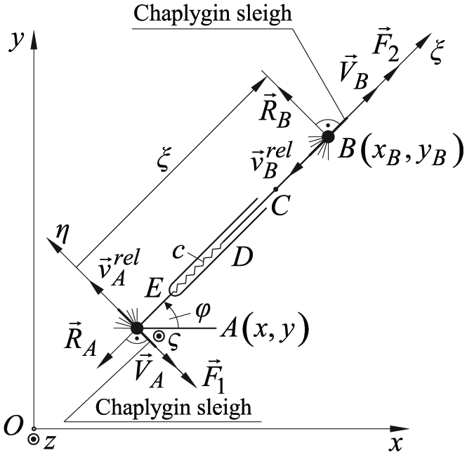
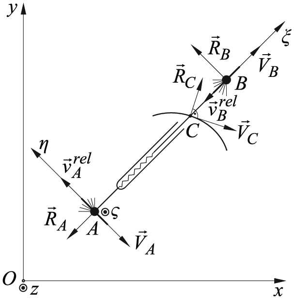
A nonholonomic mechanical system is composed of two variable-mass particles A and B, with a restriction imposed on motion in the form of the perpendicularity of velocities by means of the Chaplygin blades of negligible masses, as shown in Figure 1. For the needs of further consideration, it is necessary first to introduce two Cartesian coordinate systems of reference. The stationary coordinate system $Oxyz$ , whose coordinate plane $Oxy$ coincides with the horizontal plane of the system motion, and the moving coordinate system $A ξ η ς$ , whose coordinate origin coincides with particle A of the system, so that the coordinate plane $A ξ η$ coincides with the plane $Oxy$ . The axis of the moving coordinate system $A ξ$ is defined by the direction $AB$ , and $B \in A ξ$ , whereas the unit vectors of the axes of the moving coordinate system are $\vec{λ}, \vec{μ}$ and $\vec{ν}$ , respectively. The variable-mass particles $A$ and $B$ , as well as the spring of stiffness $c$ and free length $l_{0}$ , are interconnected by a lightweight mechanism of the “forks” type, which allows the distance $\bar{AB} = ξ \neq const .$ to change. This example is a modified version of the example considered in [8]. Namely, modification involves the addition of the spring of stiffness $c$ .

Figure 1.

Nonholonomic variable-mass mechanical system.

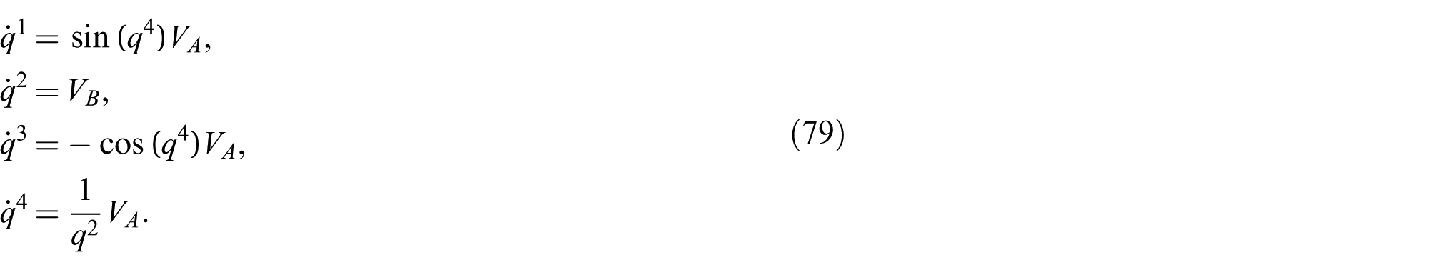
The configuration of the system considered is defined by the set of Lagrange coordinates $q = {(q^{1}, q^{2}, q^{3}, q^{4})}^{T}$ , where $q^{1} \overset{Δ}{=} x$ and $q^{3} \overset{Δ}{=} y$ are Cartesian coordinates of the particle A, $q^{4} \overset{Δ}{=} φ$ is the angle between the axis $Ox$ and axis $A ξ$ , while $q^{2} \overset{Δ}{=} ξ$ is a relative coordinate of the particle B relative to the moving coordinate system.

The laws of mass variation of particles A and B read

\begin{matrix} m_{A} (t) = m_{0} e^{- k_{A} t}, \\ m_{B} (t) = m_{0} e^{- k_{B} t}, \end{matrix}

(75)

where $m_{0}$ is the mass of particles A and B at the initial time moment $t_{0} = 0$ , and $k_{A}$ and $k_{B}$ are specified positive constants. The intensities of relative velocities of expelled masses, without loss of generality, are constant and mutually equal

v_{A}^{rel} = v_{B}^{rel} = v,

(76)

where $v$ is a specified positive constant, where ${\vec{v}}_{A}^{rel} = ν \vec{μ}$ and ${\vec{v}}_{B}^{rel} = - ν \vec{λ}$ .

Compliant with the restriction of motion of particles A and B of the system, nonholonomic homogeneous constraints can be written, in accordance with (5), in the following form

\begin{matrix} ψ^{3} \equiv {\overset{\cdot}{q}}^{1} \cos (q^{4}) + {\overset{\cdot}{q}}^{3} \sin (q^{4}) = 0, \\ ψ^{4} \equiv - {\overset{\cdot}{q}}^{1} \sin (q^{4}) + {\overset{\cdot}{q}}^{3} \cos (q^{4}) + q^{2} {\overset{\cdot}{q}}^{4} = 0 . \end{matrix}

(77)

Due to imposed restrictions of motion (77) there occur horizontal reactions of nonholonomic constraints ${\vec{R}}_{A} = - R_{A} \cos (q^{4}) \vec{i} - R_{A} \sin (q^{4}) \vec{j}$ and ${\vec{R}}_{B} = - R_{B} \sin (q^{4}) \vec{i} + R_{B} \cos (q^{4}) \vec{j}$ in particles A and B, respectively.

For independent quasi-velocities, the velocities of particles A and B are taken

\begin{matrix} {\overset{\cdot}{π}}^{1} = V_{A} = {\overset{\cdot}{q}}^{1} \sin (q^{4}) - {\overset{\cdot}{q}}^{3} \cos (q^{4}), \\ {\overset{\cdot}{π}}^{2} = V_{B} = {\overset{\cdot}{q}}^{2} . \end{matrix}

(78)

According to (8), (77) and (78), all generalized velocities can be expressed as a function of independent quasi-velocities

\begin{matrix} {\overset{\cdot}{q}}^{1} = \sin (q^{4}) V_{A}, \\ {\overset{\cdot}{q}}^{2} = V_{B}, \\ {\overset{\cdot}{q}}^{3} = - \cos (q^{4}) V_{A}, \\ {\overset{\cdot}{q}}^{4} = \frac{1}{q^{2}} V_{A} . \end{matrix}

(79)

Kinetic and potential energy of the system, according to (9) and (11), are of the form

T^{*} = \frac{1}{2} (m_{A} V_{A}^{2} + m_{B} V_{B}^{2}), Π = \frac{1}{2} c [{(q^{2} - l_{0} - L)}^{2} - {(q^{2} (t_{0}) - l_{0} - L)}^{2}],

(80)

where $L = \bar{AE} + \bar{BD}$ .

Particles A and B, respectively, are acted on by the control forces ${\vec{F}}_{1} = - F_{1} (t) \vec{μ}$ and ${\vec{F}}_{2} = F_{2} (t) \vec{λ}$ whose total power during brachistochronic motion equals zero, that is $F_{1} V_{A} + F_{2} V_{B} = 0$ .

Now, based on (18), (19), (22), (23), (29), (70), (78), (79) and (80), the differential equations of the system motion can be created

\begin{matrix} m_{A} {\overset{\cdot}{V}}_{A} = k_{A} m_{A} v + F_{1}, \\ m_{B} {\overset{\cdot}{V}}_{B} = - c (q^{2} - l_{0} - L) + k_{B} m_{B} v + F_{2} . \end{matrix}

(81)

Also, based on (21), (33) and (81), relations $Φ_{1}$ and $Φ$ are of the form

\begin{matrix} Φ_{1} = - \frac{m_{A}}{m_{B}} \frac{V_{A}}{V_{B}}, \\ Φ = k_{A} \frac{m_{A}}{m_{B}} \frac{V_{A}}{V_{B}} v + k_{B} v - \frac{c}{m_{B}} (q^{2} - l_{0} - L), \end{matrix}

(82)

therefore, according to (32), ${\overset{\cdot}{V}}_{B}$ can be expressed in the following form

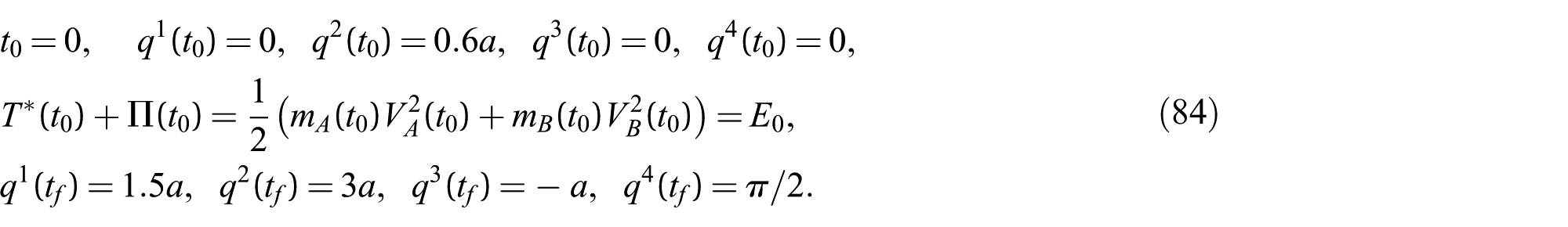
{\overset{\cdot}{V}}_{B} = k_{A} \frac{m_{A}}{m_{B}} \frac{V_{A}}{V_{B}} v + k_{B} v - \frac{c}{m_{B}} (q^{2} - l_{0} - L) - \frac{m_{A}}{m_{B}} \frac{V_{A}}{V_{B}} {\overset{\cdot}{V}}_{A} .

(83)

The initial and terminal conditions (34), (35) and (36) are known

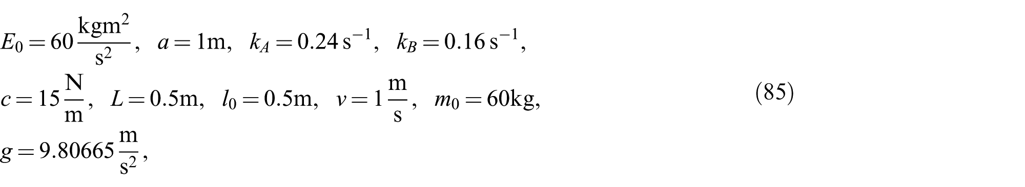
\begin{matrix} t_{0} = 0, q^{1} (t_{0}) = 0, q^{2} (t_{0}) = 0.6 a, q^{3} (t_{0}) = 0, q^{4} (t_{0}) = 0, \\ T^{*} (t_{0}) + Π (t_{0}) = \frac{1}{2} (m_{A} (t_{0}) V_{A}^{2} (t_{0}) + m_{B} (t_{0}) V_{B}^{2} (t_{0})) = E_{0}, \\ q^{1} (t_{f}) = 1.5 a, q^{2} (t_{f}) = 3 a, q^{3} (t_{f}) = - a, q^{4} (t_{f}) = π / 2 . \end{matrix}

(84)

Using the numerical procedure from Section 3, the TPBVP (63) and (84) has been solved for the following values of the parameters

\begin{matrix} E_{0} = 60 \frac{kg m^{2}}{s^{2}}, a = 1 m, k_{A} = 0.24 s^{- 1}, k_{B} = 0.16 s^{- 1}, \\ c = 15 \frac{N}{m}, L = 0.5 m, l_{0} = 0.5 m, v = 1 \frac{m}{s}, m_{0} = 60 kg, \\ g = 9.80665 \frac{m}{s^{2}}, \end{matrix}

(85)

therefore, relation (62) now has the form

λ_{2} (t_{f}) = \frac{m_{B} (t_{f}) V_{B} (t_{f})}{m_{A} (t_{f}) {(V_{A} (t_{f}))}^{2} + m_{B} (t_{f}) {(V_{B} (t_{f}))}^{2}} .

After the numerical procedure is carried out, the following functions are obtained in the numerical form

q^{1} (t), q^{2} (t), q^{3} (t), q^{4} (t), V_{A} (t), V_{B} (t), λ_{2} (t), λ_{3} (t), λ_{4} (t), ν_{2} (t),

(86)

as well as the time of brachistochronic motion $t_{f} = 1.98649 s .$

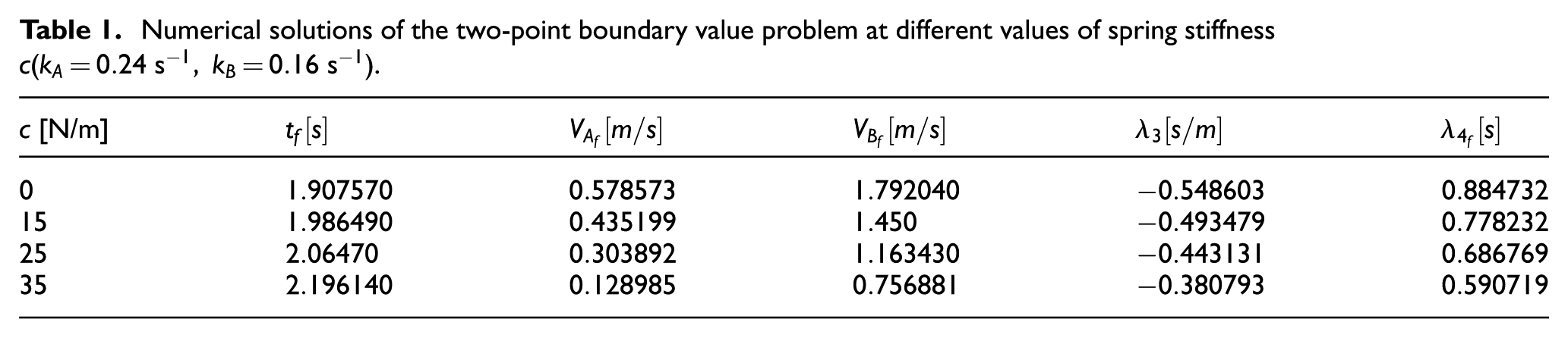
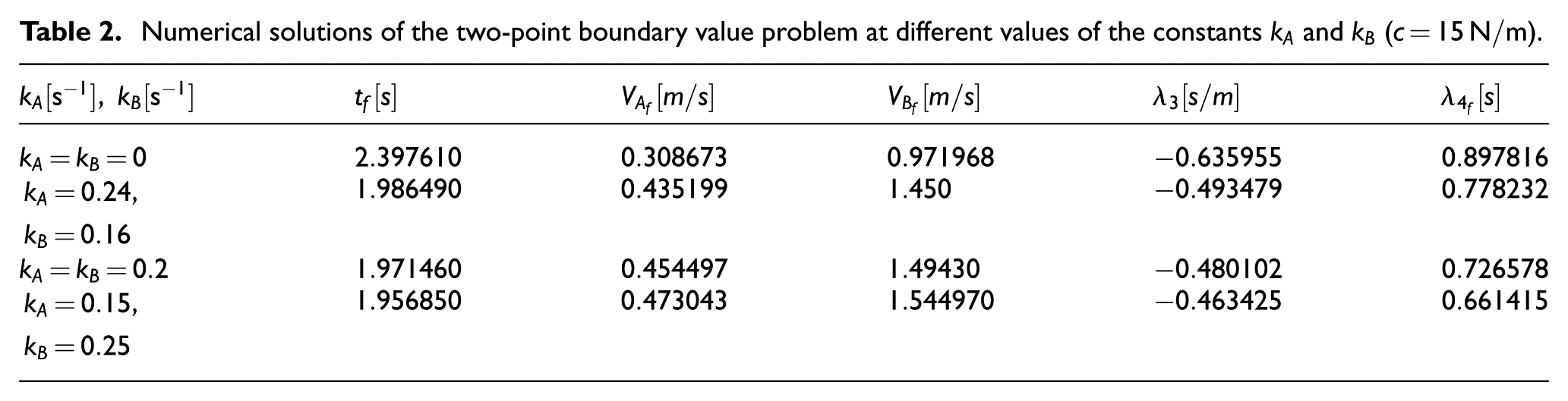
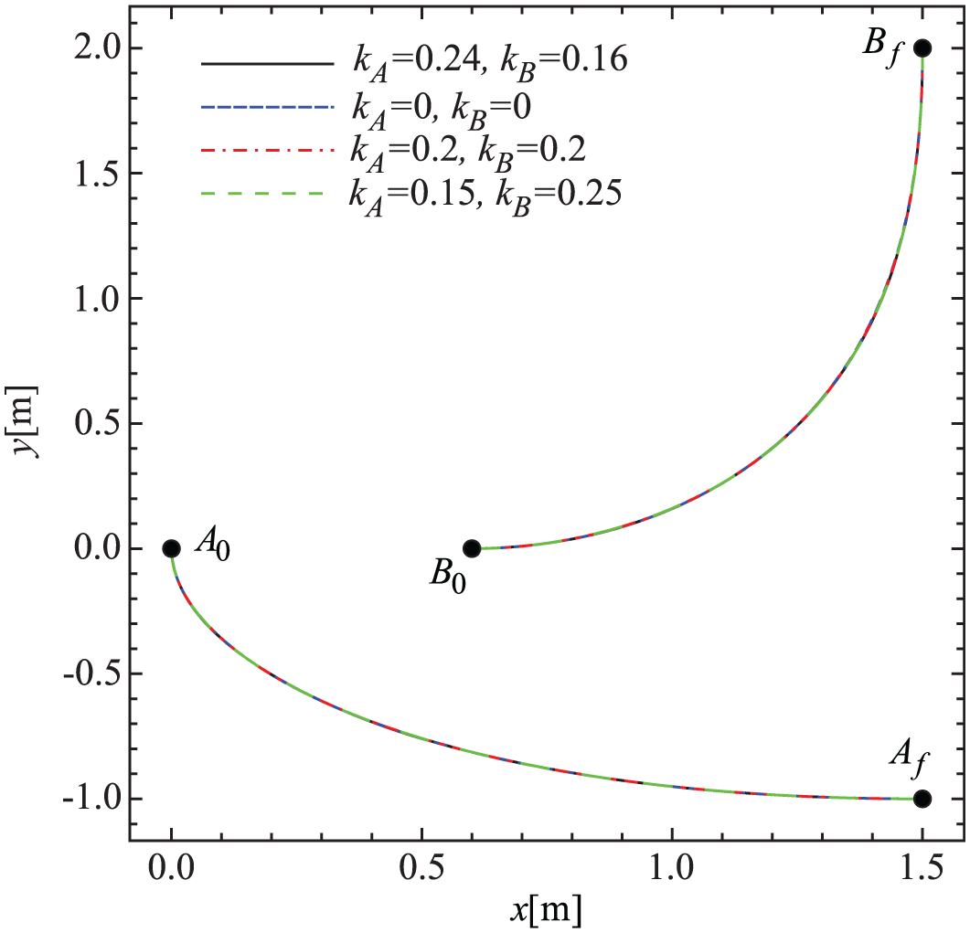
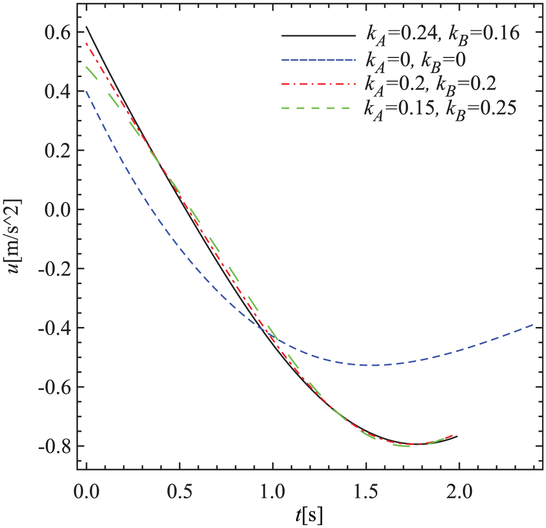
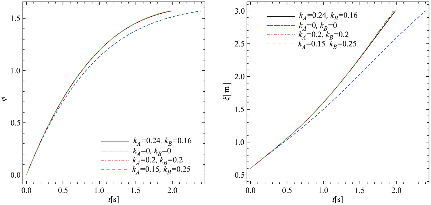
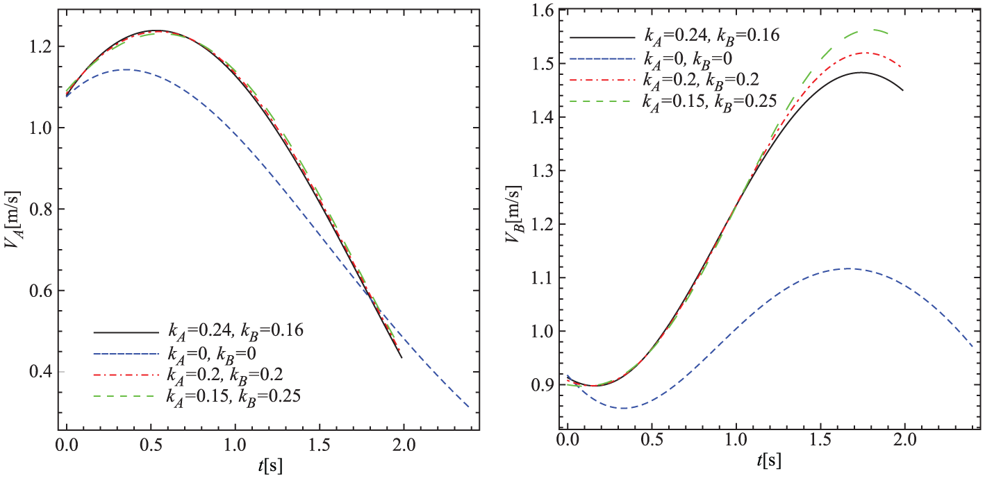
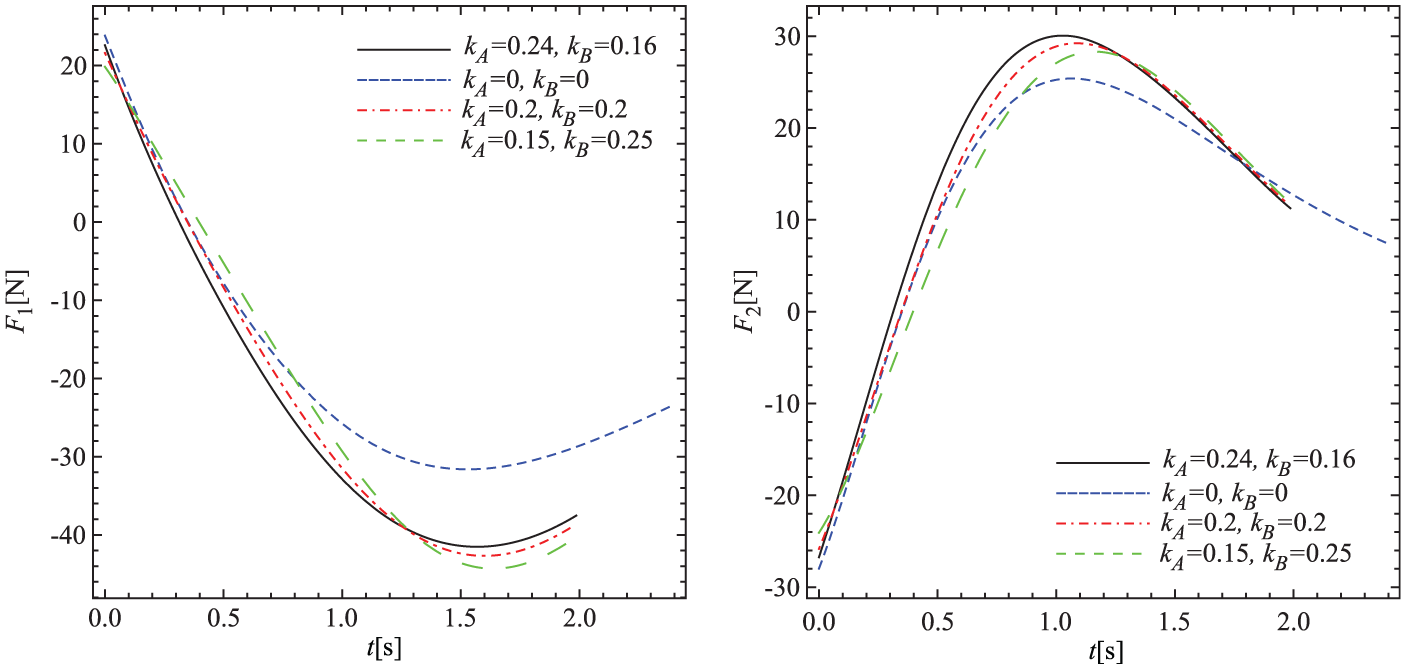
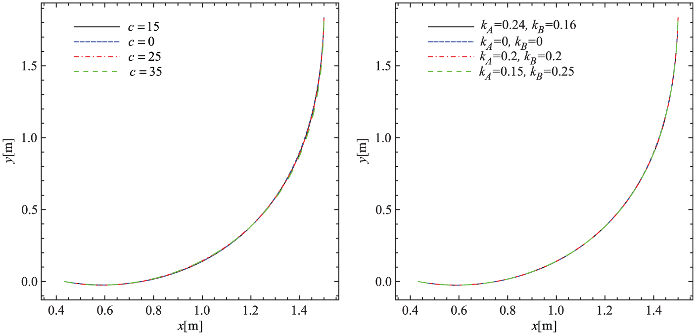
For different values of the spring stiffness $c$ , Table 1 shows the missing boundary values at the values of constants $k_{A} = 0.24 s^{- 1}$ and $k_{B} = 0.16 s^{- 1}$ . Furthermore, it can be clearly seen that as the value of spring stiffness increases, minimum time $t_{f}$ also increases. Table 2 displays the missing boundary values at different values of the constants $k_{A}$ and $k_{B}$ and the spring stiffness value $c = 15 N / m$ . Figures 2 –7 give comparative graphical representation of the results at different values of constants $k_{A}$ and $k_{B}$ and the spring stiffness value $c = 15 N / m$ . Figure 2 shows the trajectories of points A and B, whereas Figure 3 depicts the law of variation of the control $u (t) = {\overset{\cdot}{V}}_{A} (t)$ . Graphs of the generalized coordinates $q^{2} (t) = ξ (t)$ and $q^{4} (t) = φ (t)$ are given in Figure 4, whereas the law of variation of velocities $V_{A} (t)$ and $V_{B} (t)$ is shown in Figure 5.

Table 1.

Numerical solutions of the two-point boundary value problem at different values of spring stiffness $c$ ( $k_{A} = 0.24 s^{- 1}, k_{B} = 0.16 s^{- 1}$ ).

$c$ [N/m]	$t_{f} [s]$	$V_{A_{f}} [m / s]$	$V_{B_{f}} [m / s]$	$λ_{3} [s / m]$	$λ_{4_{f}} [s]$
0	$1.907570$	$0.578573$	$1.792040$	$- 0.548603$	$0.884732$
15	$1.986490$	$0.435199$	$1.450$	$- 0.493479$	$0.778232$
25	$2.06470$	$0.303892$	$1.163430$	$- 0.443131$	$0.686769$
35	$2.196140$	$0.128985$	$0.756881$	$- 0.380793$	$0.590719$

Table 2.

Numerical solutions of the two-point boundary value problem at different values of the constants $k_{A}$ and $k_{B}$ ( $c = 15 N / m$ ).

$k_{A} [s^{- 1}], k_{B} [s^{- 1}]$	$t_{f} [s]$	$V_{A_{f}} [m / s]$	$V_{B_{f}} [m / s]$	$λ_{3} [s / m]$	$λ_{4_{f}} [s]$
$k_{A} = k_{B} = 0$	$2.397610$	$0.308673$	$0.971968$	$- 0.635955$	$0.897816$
$\begin{matrix} k_{A} = 0.24, \\ k_{B} = 0.16 \end{matrix}$	$1.986490$	$0.435199$	$1.450$	$- 0.493479$	$0.778232$
$k_{A} = k_{B} = 0.2$	$1.971460$	$0.454497$	$1.49430$	$- 0.480102$	$0.726578$
$\begin{matrix} k_{A} = 0.15, \\ k_{B} = 0.25 \end{matrix}$	$1.956850$	$0.473043$	$1.544970$	$- 0.463425$	$0.661415$

Figure 2.

Trajectories of points A and B.

Figure 3.

Graph of the control u(t).

Figure 4.

Graphs of the angle $φ$ and the relative coordinate $ξ$ .

Figure 5.

Graphs of the velocities $V_{A}$ and $V_{B}$ .

Figure 6.

Graphs of the control forces $F_{1} (t)$ and $F_{2} (t)$ .

Figure 7.

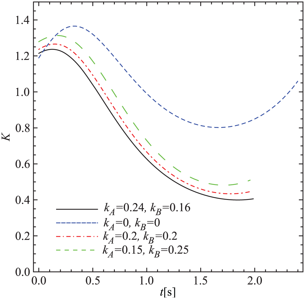
Numerical confirmation of the Kelley optimality condition (88).

According to (71), the control forces $F_{1}$ and $F_{2}$ can now be expressed in the following form

F_{1} = m_{A} (u - k_{A} ν), F_{2} = - m_{A} \frac{V_{A}}{V_{B}} (u - k_{A} ν),

(87)

whose graphs are given in Figure 6.

The control u, whose law of variation is shown in Figure 3, represents the first-order singular control. The necessary Kelley optimality condition for the first-order singular control is

- \frac{\partial}{\partial u} (\frac{d^{2}}{d t^{2}} [\frac{\partial H}{\partial u}]) \leq 0,

(88)

which can be represented in the following form

\begin{matrix} K \equiv \frac{\partial}{\partial u} (\frac{d^{2}}{d t^{2}} [\frac{\partial H}{\partial u}]) = \frac{1}{m_{0} V_{B}^{4}} e^{2 (- k_{A} + k_{B}) q^{5}} (m_{0} λ_{2} V_{B} (V_{A}^{2} + e^{(k_{A} - k_{B}) q^{5}} V_{B}^{2}) + \\ ν_{2} ((e^{k_{B} q^{5}} c (L + l_{0}) + k_{B} m_{0} ν - e^{k_{B} q^{5}} c q^{2}) V_{A}^{2} + \\ e^{(k_{A} - k_{B}) q^{5}} V_{B}^{2} (e^{k_{B} q^{5}} cL + e^{k_{B} q^{5}} c l_{0} + k_{B} m_{0} ν - e^{k_{B} q^{5}} c q^{2} + (k_{A} - k_{B}) m_{0} V_{B}))) \geq 0 . \end{matrix}

(89)

Figure 7 presents the law of variation of function K from (89), at different values of the constants $k_{A}$ and $k_{B}$ and the spring stiffness value $c = 15 N / m$ , which leads to a straightforward conclusion that condition (88) is fulfilled.

Another possible way of realizing the motion of the considered 2DOF system is to subsequently impose to the system one holonomic stationary ideal independent mechanical constraint in accordance with previously defined brachistochronic motion but without the action of control forces. The mechanical constraint has been realized by means of a smooth guide whose pathline coincides with the point C trajectory, which is located at the distance $\bar{BC} = 1 / 6 m$ , so that the parametric equations are the guide lines

\begin{matrix} x_{C} (t) = q^{1} + (q^{2} - \bar{BC}) \cos (q^{4}), \\ y_{C} (t) = q^{3} + (q^{2} - \bar{BC}) \sin (q^{4}) . \end{matrix}

(90)

In Figure 8, ${\vec{R}}_{C}$ represents a subsequently imposed mechanical constraint – smooth guide, where ${\vec{R}}_{C} \cdot {\vec{V}}_{C} = 0$ . Figure 9 presents the trajectories of point C at different spring stiffness values and different values of the constants $k_{A}$ and $k_{B}$ .

Figure 8.

Realization of the system brachistochronic motion by means of a smooth guide.

Figure 9.

Trajectories of point C at different spring stiffness values $c$ and different values of the constants $k_{A}$ and $k_{B}$ .

6. Conclusions

In this paper, the problem of brachistochronic motion of a variable-mass nonholonomic mechanical system has been solved. The paper represents the generalization of the results obtained in [8] to the general variable-mass systems with linear nonholonomic constraints and $m$ degrees of freedom. Taking the first time-derivatives of quasi-velocities as control variables, the brachistochrone problem considered has been formulated as a singular optimal control task. The results obtained may be used as a base for further researches in the field of minimum time control of mechanical systems composed of variable-mass bodies (for such mechanical systems in engineering practice, see [10 –12]).

Footnotes

Funding

Support for this research was provided by the Ministry of Education, Science and Technological Development of the Republic of Serbia under Grants Nos. ON17400 and TR35006. This support is gratefully acknowledged.

References

Chang

. Extended Kane’s equations for nonholonomic variable mass system. J Appl Mech (Trans ASME) 1982; 49: 429-431.

. The equations of motion of nonlinear nonholonomic variable mass system with applications. J Appl Mech (Trans ASME) 1984; 51: 435-437.

Qiao

. Gibbs-Appell’s equations of variable mass nonlinear nonholonomic mechanical systems. Appl Math Mech Engl 1990; 11: 973-983.

Cheng

. The Hamilton’s principle of nonholonomic variable mass systems. Appl Math Mech Engl 1983; 4: 291–302.

Luo

Zhao

. Routh’s equations for general nonholonomic mechanical systems of variable mass. Appl Math Mech Engl 1993; 14: 285-298.

Apykhtin

Yakovlev

. On the motion of dynamically controlled systems with variable masses.PMM J Appl Math Mec+ 1980; 44: 301–305.

Azizov

. On the motion of a controlled system of variable mass.PMM J Appl Math Mec+ 1986; 50: 433-437.

Jeremić

Radulović

Obradović

. Analysis of the brachistochronic motion of a variable mass nonholonomic mechanical system. Theor Appl Mech 2016; 43: 19–32.

Obradović

Šalinić

Jeremić

et al . On the brachistochronic motion of a variable-mass mechanical system in general force fields. Math Mech Solids 2014; 19: 398-410.

10.

Cvetićanin

. Dynamics of machines with variable mass. Amsterdam: Gordon and Breach Science Publishers, 1998.

11.

Cvetićanin

. Dynamics of bodies with time-variable mass. New York: Springer, 2016.

12.

Irschik

Belyaev

(eds). Dynamics of mechanical systems with variable mass. New York: Springer, 2014.

13.

Lurie

. Analytical mechanics. Berlin Heidelberg: Springer, 2002.

14.

Papastavridis

. Analytical mechanics. New York: Oxford University Press, 2002.

15.

Papastavridis

. Tensor calculus and analytical dynamics. Boca Raton, FL: CRC Press, 1999.

16.

Baird

Hughes

RIG

Nordmann

(eds). Heinrich Hertz: classical physicist, modern philosopher. Dordrecht: Kluwer Academic, 1998.

17.

Vujanović

Atanacković

. An introduction to modern variational techniques in mechanics and engineering. Boston, MA: Birkhäuser, 2004.

18.

Cvetićanin

. Conservation laws in systems with variable mass. J Appl Mech (Trans ASME) 1993; 60: 954-958.

19.

Pesce

. The application of Lagrange equations to mechanical systems with mass explicitly dependent on position. J Appl Mech (Trans ASME) 2003; 70: 751–756.

20.

Čović

Vesković

. Brachistochronic motion of a multibody system with Coulomb friction. Eur J Mech A Solid 2009; 28: 882–890.

21.

Geering

. Optimal control with engineering applications. Berlin Heidelberg: Springer-Verlag, 2007.

22.

Pontryagin

Boltyanskii

Gamkrelidze

et al . The mathematical theory of optimal processes. New York: Interscience, 1962.

23.

Gabasov

Kirillova

. High order necessary conditions for optimality. SIAM J Control 1972; 10: 127–168.

24.

Stoer

Bulirsch

. Introduction to numerical analysis. New York: Springer, 1993.

25.

Bertolazzi

Biral

Da Lio

. Symbolic-numeric efficient solution of optimal control problems for multibody systems. J Comput Appl Math 2006; 185: 404-421.

26.

Wolfram

. The Mathematica book. 5th ed. Champaign, IL: Wolfram Media, 2003.

27.

Abell

Braselton

. Differential equations with Mathematica. 3rd ed. Amsterdam: Elsevier Academic Press, 2004.