This work is concerned with a recent thermoelastic model. We investigate the propagation of plane harmonic waves in the context of this very recently proposed heat conduction model, an exact heat conduction model with a single delay term, established by Quintanilla. This model attempted to reformulate the heat conduction model that takes into account microstructural effects in heat transport phenomena and provided an alternative heat conduction theory with a single delay term. We aim to study the harmonic plane waves propagating in a thermoelastic medium by employing this new model and derive the exact dispersion relation solution. We mainly focus on a longitudinal wave coupled to a thermal field and find two different modes of this wave. We derive asymptotic expressions for several important characterizations of the wave fields: phase velocity, specific loss, penetration depth, and amplitude ratio. Analytical expressions for these wave characteristics are obtained for different cases of very-high- and low-frequency regions for elastic- and thermal-mode longitudinal waves. To verify the analytical results, we also carry out computational work to obtain numerical results of the wave characterizations for intermediate values of frequency and illustrate the results graphically. We show that our analytical and numerical results are in perfect match. On the basis of the analytical and numerical results, a thorough analysis of the effects of the single delay parameter on various wave characteristics is presented. We highlight several characteristic features of the new thermoelastic model, as compared with other models.
Biot [1] introduced the theory of coupled thermoelasticity based on Fourier’s law. Fourier’s famous law of heat conduction presents a linear relationship between the heat flux (q) through a material and the gradient of temperature (T). In principle, Fourier’s law leads to a nonphysical infinite heat propagation speed within a continuum field for transient heat conduction processes because of its parabolic characteristics, which is in contradiction with the theory of relativity. To overcome this contradiction, several non-Fourier heat constitutive models have been introduced, which have drawn serious attention from researchers. Subsequently, modifications of the theory of thermoelasticity have been made and have given rise to new theories, which are referred as generalized thermoelasticity theories or hyperbolic thermoelasticity theories.
Lord and Shulman [2] developed the first generalized theory of thermoelasticity by introducing a time (t) dependent term, the relaxation time, based on the Cattaneo–Vernotte heat conduction model [3–5]. Later on, Green and Lindsay [6] introduced an explicit version of the constitutive equations involved in coupled thermoelasticity. In this theory, all the equations are modified by involving two constants in the constitutive equations that act as thermal relaxation time parameters. Basic governing equations of both these generalized theories are of hyperbolic type and confirm the finite speed of thermal waves.
Next, early in 1990, Green and Naghdi [7–9] proposed another new generalized thermoelasticity theory on the basis of energy balance and entropy balance. This theory considers thermal displacement as a constitutive variable in addition to temperature. Green and Naghdi [7–9] divided their theory into three parts, which are subsequently referred to as thermoelasticity of types I, II, and III. When the theory of type I is linearized, the parabolic equation of heat conduction arises (the theory based on Fourier’s law), whereas the linearized version of type II permits propagation of thermal waves with finite speed, which is more suitable from a physical point of view. The heat conduction law for the GN-III model is of the more general form, as
In this theory, the gradients of thermal displacement () and temperature (T) are considered as the constitutive variables, where the thermal displacement satisfies . The two positive constants k and are the thermal conductivity and the conductivity rate, respectively; (of physical dimensions conductivity per time) is a material constant and a characteristic of the theory.
Afterward, to incorporate the microscopic effects into a microscopic description, Tzou [10] developed a phenomenological hyperbolic model for the ultra fast heating process, termed a dual-phase-lag model. The form of heat conduction law for this model, relating q at a point P to at P, is
Here, and are termed the phase-lags of the heat flux and temperature gradient, respectively. The time lags are assumed to be positive and are intrinsic properties of the medium [10, 11].
Subsequently, Roychoudhuri [12] has established a generalized mathematical model of coupled thermoelasticity theory that includes three-phase-lags, in the heat flux vector, the temperature gradient, and the thermal displacement gradient. The model formulated is an extension of the thermoelastic models proposed by Lord and Shulman [2], Green and Naghdi [7–9] and Tzou [10, 11]. According to this model, the constitutive equation for the heat flux vector has been modified as
Here is the additional delay time, known as the phase-lag of the thermal displacement gradient.
The thermoelasticity theories discussed here have drawn serious attention from researchers over the years and they observe distinctive features of various models. Some critical analysis of these theories has also been discussed. For example, Dreher et al. [13] have reported a critical analysis of the dual phase-lag and three-phase-lag heat conduction models and explained that when the constitutive equation is adjoined with an energy equation,
we always get a sequence of eigenvalues in the point spectrum, such that its real parts tend to infinity [13]. This result shows the instability of the problem. Moreover, it says that the associated mathematical problem is ill-posed. That is, we cannot obtain continuous dependence of the solution with respect to initial parameters. The mathematical consequences of such theories do not agree with what one would have previously expected [13]. For this reason, much interest has been paid to a study of the different Taylor series approximations to these heat conduction equations, where we get continuous dependence and stability [14–21]. Recently, Quintanilla [22] has reformulated the three-phase-lag model in an alternative way and examined the stability and spatial behavior of the new proposed model. By defining and , and combining equation (3) with the energy equation (equation (4)) defines a well-posed problem. That is, a well-posed problem in the context of the exact three-dual-phase theory. The field equation of this new model with a single delay term is of the form
Here, is the Laplacian operator. Subsequently, Leseduarte and Quintanilla [23] have examined this reformulated model in a precise manner. A Phragmén–Lindelöf-type alternative is obtained; it has been shown that the solutions either decay exponentially or increase to infinity exponentially. The obtained results are extended to a thermoelasticity theory by considering the Taylor series approximation of the equation of heat conduction to the delay term and a Phragmén–Lindelöf type alternative is obtained for equations acting both forward and backward in time. Recently, Kumari and Mukhopadhyay [24] established the uniqueness of the solution of this theory [22, 23]. They also discussed the variational principle and reciprocity theorem of this model. A uniqueness theorem and instability of solutions under the relaxed assumption that the elasticity tensor can be negative is established by Quintanilla [25]. Kumar and Mukhopadhyay [26] investigated a problem of thermoelastic interactions on this theory, in which a state-space approach is used to formulate the problem and the formulation is then applied to a problem of an isotropic elastic half-space, with its plane boundary subjected to a sudden increase in temperature and zero stress.
The propagation of harmonic plane waves in classical thermoelasticity was studied by Lessen [27], Deresiewicz [28], Chadwick and Sneddon [29] and Chadwick [30]. Later on, Nayfeh and Nemat-Nasser [31] and Puri [32] analyzed the propagation of plane waves in the context of Lord-Shulman theory, i.e., under the generalized thermoelasticity theory with one relaxation time. The propagation and stability of harmonically time-dependent thermoelastic plane waves in temperature-rate-dependent thermoelasticity was reported by Agarwal [33]. Wave propagation in the Green-Lindsay and Lord-Shulman models has again been studied by Haddow and Wegner [34]. Plane waves are discussed by Chandrasekharaiah [35] with reference to the thermoelasticity theory of the GN-II model. Prasad et. al. [36] examined the propagation of plane waves under thermoelasticity with dual-phase-lags. Puri and Jordan [37] and Kothari and Mukhopadhyay [38] explored the propagation of plane waves in GN-III thermoelastic theory.
The aim of this paper is to interpret the propagation of plane harmonic waves in a homogeneous and isotropic unbounded medium in the context of the new proposed thermoelastic model given by Quintanilla [22]. After mathematical formulation of the problem, we obtain the dispersion relation for a longitudinal plane wave. Two distinct modes of longitudinal plane wave have been identified. An analytical solution of the dispersion relation is obtained. We further find the asymptotic expansions of several qualitative characterizations of the wave field, such as phase velocity, specific loss, and penetration depth for the high- and low-frequency values for this model. The amplitude ratio of thermal and elastic waves is investigated. To verify the analytical results predicting the limiting behavior of the wave characteristics, we carry out computational work and obtain numerical values of the wave characteristics for intermediate values of frequency. We show a perfect match in the analytical and numerical results. We highlight some specific features of the model of thermoelasticity that was introduced recently [22]. We believe that the findings of this work may be useful in understanding the applicability of this new model.
2. Basic governing equations
We consider an unbounded, isotropic, and thermally conducting elastic medium. The constituent equations and basic governing equations for the thermoelastic interactions inside the medium in the absence of body forces and heat sources, in the context of the new thermoelastic model given by Quintanilla [22, 23] are considered as follows:
Stress–strain–temperature relation.
Strain–displacement relation.
Equation of motion without body force.
The displacement equation of motion without body force is obtained from equations (6)–(8) as
The heat conduction equation in the context of new model given by Quintanilla [23] is taken in the form
Here, we measure the displacement vector from a steady-state position and the deformation is supposed to be very small. In these equations, the partial derivative with respect to the space variables is denoted by the comma notations and the partial derivative with respect to time is represented by dot operators. are the components of the stress tensor, are the components of the strain tensor, is the absolute temperature, is the reference temperature, is a component of the displacement vector, and k and are the thermal conductivity and the rate of thermal conductivity of the material, respectively. is the specific heat capacity at constant strain, is a delay term in the context of the new model, and are Lamé elastic constants, , where is the coefficient of linear thermal expansion. The parameter has been used here to formulate the problem under three different models of heat conduction in a unified way. The case when we assume in equation (10) corresponds to the heat conduction equation of thermoelasticity under the GN-III model. In the case when , we obtain two different versions of heat conduction equation, introduced by Quintanilla (equation (27)) and Quintanilla and Leseduarte (equation (28)) by assuming and . Here, in the second case (i.e., when ), the second-order effect is neglected in the Taylor series approximation of the equation of heat conduction to the delay term, .
Hence, we study our problem by considering equations (9) and (10) to analyze the results under three different cases, as follows:
New model I.;
New model II.;
GN-III model..
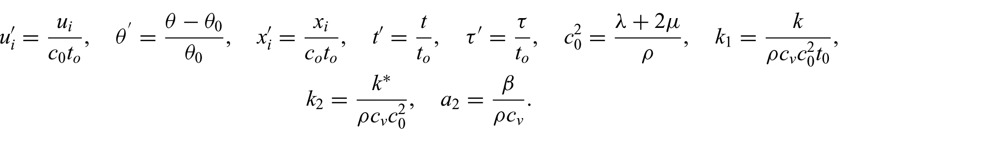
To make equations (9) and (10) simpler, we use the following dimensionless transformations:
Here, is the characteristic response in time for the medium.
Now, after dropping the primes for convenience, equations (9) and (10) change to the following forms:
We will study our problem in the contexts of three models simultaneously on the basis of these two equations.
3. Dispersion relation and its derivation
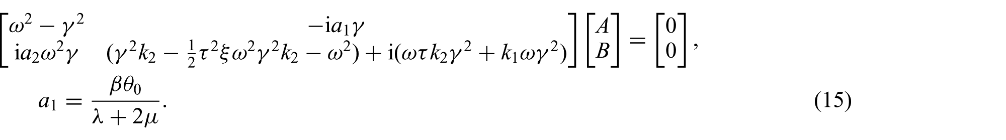
The transverse wave remains uncoupled from the thermal field of the medium, whereas, in the case of the longitudinal wave, the mechanical and thermal fields are coupled together. Therefore, we omit the analysis of the transverse wave and we focus on the longitudinal wave. We are therefore considering the solution of a longitudinal plane wave of the form
where is a positive real number called the angular frequency of the wave and is a complex constant. A and B are complex amplitudes (simultaneously not both zero). Here, is the unit vector in the direction of displacement and is the unit vector normal to the wave front. , , and are the phase velocity, frequency, and wavelength, respectively, of the longitudinal waves. For our analysis, and must hold obviously for the wave to be physically realistic.
Since, for a non-trivial solution of equation (15), the determinant of this system must be zero, we therefore obtain a bi-quadratic dispersion relation as
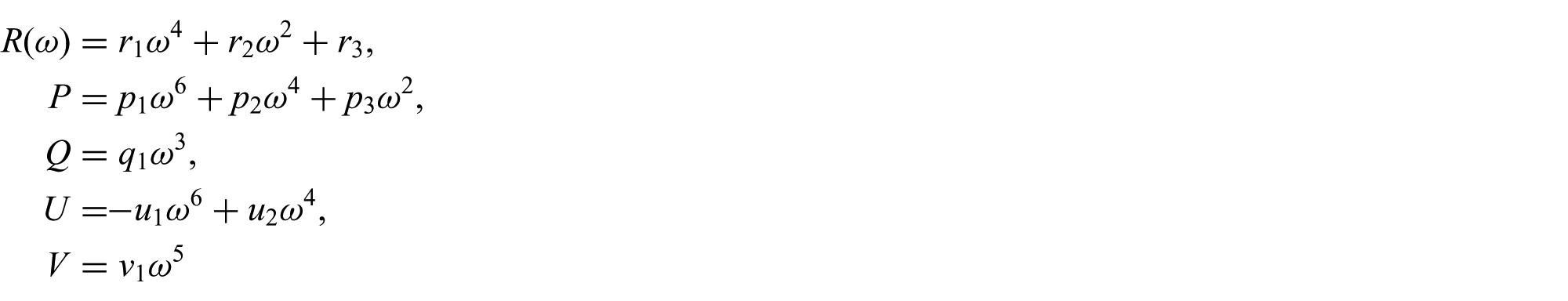
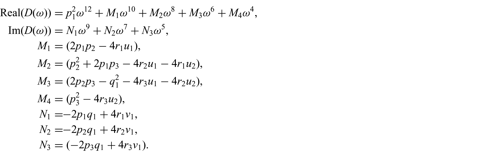
Here, we observe from equation (16) that the harmonic plane wave is clearly influenced by the delay term. Now by making the coefficient of real, we arrive at the simplified form of the dispersion relation
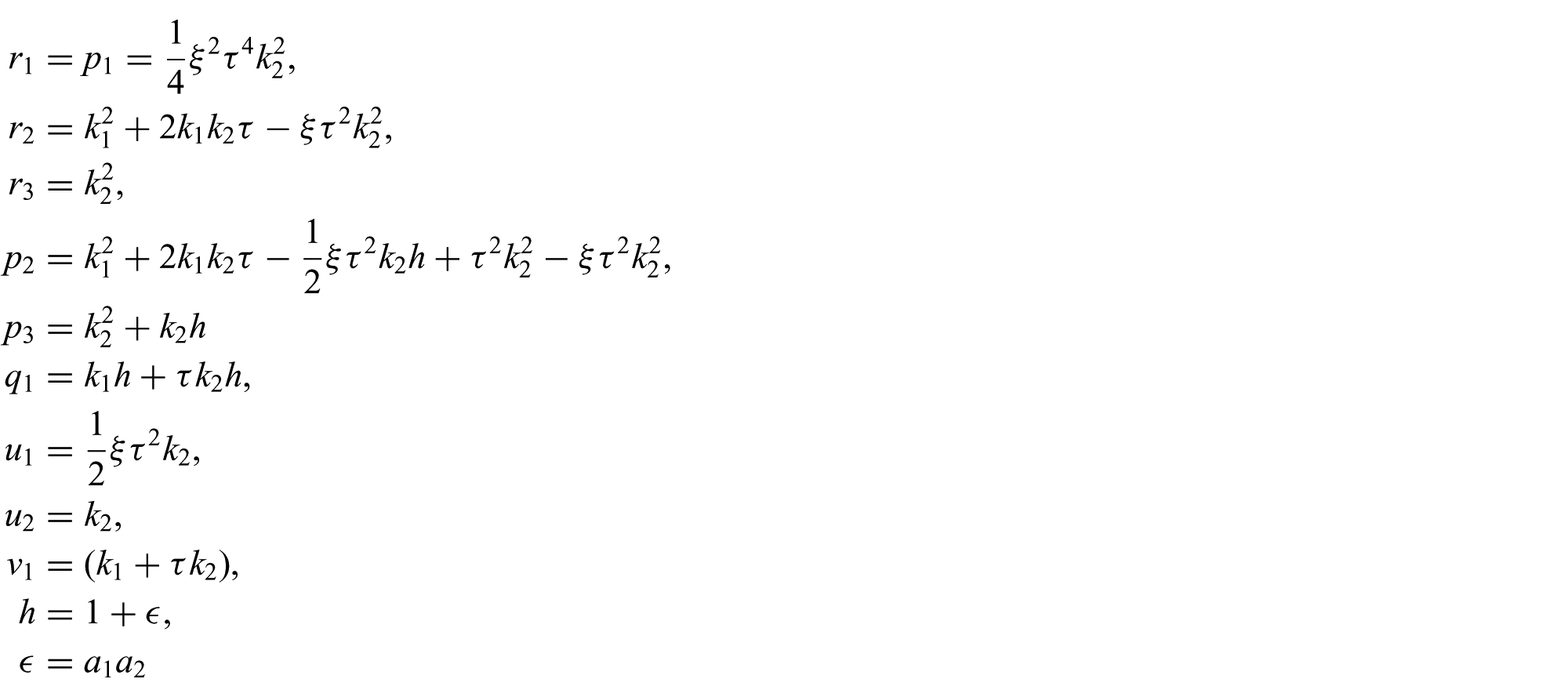
where
and
Equation (17) is therefore the unified form of the dispersion relation for new model I, new model II, and the GN-III model; it clearly shows the effects of a single delay term on the longitudinal plane waves. We observe that the dispersion relation (equation (17)) for the case when , i.e., for the GN-III model, matches perfectly with the corresponding relation derived by Puri and Jordan [37].
3.1. Solution of dispersion relation
If the roots of equation (17) are , and , then we can write
where
Here, it is to be mentioned that among the four roots of , only two have negative imaginary parts. We will consider only those two roots with negative values of decay coefficient, . Now equation (18) can be solved by applying the following theorem of complex numbers.
Theorem 1 (Ponnusamy [39]). For a given, the solutions ofare given by
Using this theorem in equation (18), we can find two values of whose imaginary parts are negative. These two values of correspond to two types of the dilational (longitudinal) wave, in which the first one is predominantly elastic, and the second is thermal in nature. We denote related to the first type by and related to the second one by .
4. Analytical results
Since the general analysis of waves on the basis of the roots given by equation (18) is highly complicated, we therefore concentrate on the analysis of waves and the effects of delay terms under two special cases, which correspond to waves of very high and very low frequency. Hence, we first obtain the asymptotic expressions for and from equation (18) by using the previous theorem under these two special cases by assuming to be very large and very small, respectively. The results for the case of the GN-III model are reported by Puri and Jordan [37]. Therefore, we skip the derivation of the analytical results of the GN-III model. For the other two models, we proceed as follows.
4.1. Case I: High-frequency asymptotic expansions
In this case, we assume to be very large, i.e., . Hence, expanding equation (18) for large and neglecting higher powers of , we can write equation (18) as
where
and
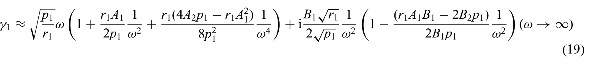
4.1.1. Analytical results for γ1,2
For large values of , expanding the equation for and neglecting higher powers of , again using the theorem of complex analysis, as mentioned, we finally obtain the asymptotic expansion of the roots of equation (18) for new model I and new model II, as follows:
for new model I.
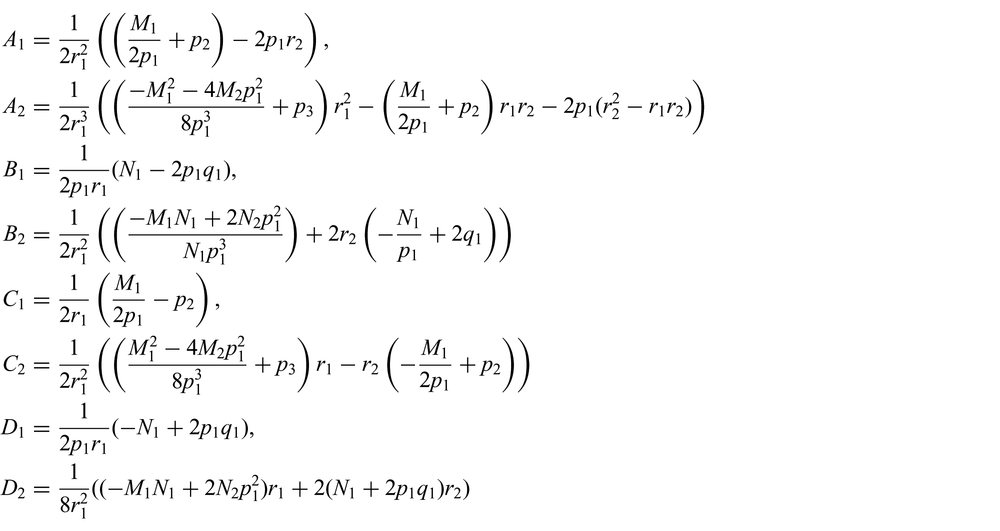
where
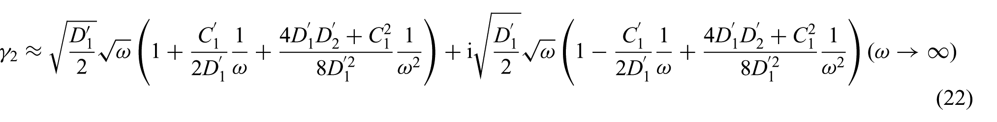
for new model II.
where
4.2. Case II: Low-frequency asymptotic expansions
We use a similar approach for the low-frequency asymptotic expressions of different wave fields, and find the required roots of equation (18) by considering to be very very small, i.e., . Interestingly, we get exactly similar results for new model I and new model II; they are obtained as follows:
for new model I and new model II.
where
5. Asymptotic results for different wave fields
Now we make an attempt to derive the asymptotic expressions of the important wave components, i.e., phase velocity, specific loss, penetration depth, and amplitude ratio, of both the modified elastic wave and thermal waves and study characteristics under the case of high-frequency values as well as low-frequency values. Here we see that in the case of low-frequency asymptotic expansion of all wave components, we get similar expressions for new model I and new model II.
5.1. Phase velocity
The phase velocity of the wave is given by the formula
where and represent the phase velocities of elastic-mode and thermal-mode waves, respectively.
With the help of equations (19) to (24), and using equation (25), we find the high-frequency and low-frequency asymptotic expressions for and as follows.
5.1.1. High-frequency asymptotes of phase velocities
New model I.
New model II.
5.1.2. Low-frequency asymptotes of phase velocities
New model I and new model II.
5.2. Specific loss
We define specific loss as the ratio of energy dissipated per stress cycle to the total vibration energy, which is given as
where are the specific losses of elastic and thermal waves, respectively.
With the help of equations (19) to (24), and using equation (32), we find the high-frequency and low-frequency asymptotic expressions for , as follows.
5.2.1. High-frequency asymptotic expansions of specific loss
New model I.
New model II.
5.2.2. Low-frequency asymptotic expansions of specific loss
New model I and new model II.
5.3. Penetration depth
We define penetration depth by the following relation:
where and are the penetration depths of elastic- and thermal-mode waves, respectively.
With the help of equations (19) to (24) and (39) we find the high-frequency and low-frequency asymptotic expressions for and from this formula, as follows.
5.3.1. High-frequency asymptotic expansions of penetration depth
New model I.
New model II.
5.3.2. Low-frequency asymptotic expansions of penetration depth
New model I and new model II.
5.4. Amplitude ratio
In view of equations (13) to (15), we find the amplitude ratios of elastic- and thermal-mode longitudinal wave as
Here, and are the amplitude ratios of elastic and thermal waves, respectively.
Now, with the help of equations (19) to (24) and (46), we find the high-frequency and low-frequency asymptotic expressions for and from the formula, as follows.
5.4.1. High-frequency asymptotes of amplitude ratios
New model I.
New model II.
5.4.2. Low-frequency asymptotes of amplitude ratios
New model I and new model II.
6. Analysis of analytical and numerical results
To interpret the asymptotic results obtained in the previous section and to look into the nature of various wave components in detail, we have made an attempt to find the numerical values of different wave characterizations for both thermal- and elastic-mode longitudinal waves. For this, we have assumed , , , and . Using the software Matlab, we have generated codes to compute the numerical values of different components directly from equation (18) and by using equations (25), (32), (39) and (46). The computation for the numerical values of phase velocity, specific loss, and penetration depth under all three cases, namely, new model I, new model II, and the GN-III model for different values of frequency, , is carried out and the results are presented in the different figures. In all the figures, we observe the variation of different wave characteristics with frequency in the contexts of these three models. Both low- and high-frequency cases are shown separately in order to show the limiting behavior of the wave fields. We also show the variations of the wave fields with the variation of thermal conductivity rate, .
6.1. Phase velocity
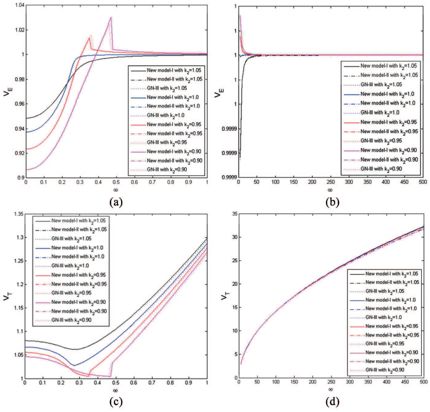
Figure 1(a) represents the variation of phase velocity of an elastic-mode wave for the low-frequency case. It shows that the phase velocity, of an elastic-mode wave, under New model I, New model II, and the GN-III model are of almost similar nature for a fixed value of . However, there is a prominent difference for different values of under each model. approaches a constant value as under each model and also for each value of . This limiting value (equal to , as is clear from the analytical result given by equation (30)) is the same for each model but is dependent on . In the case when , its value is approximately 0.9372. Interestingly, we note that for the case when , there are two corner points in the plots of , indicating the existence of two critical frequencies corresponding to these points. The location of the corner point shifts toward right as increases. For , there exist a local maxima for under each model, while in the case of , is a non-decreasing function of frequency and finally reaches a constant limiting value, which is its maximum.
(a) Variation of phase velocity of elastic wave () vs. low frequency (). (b) Variation of phase velocity of elastic wave () vs. high frequency (). (c) Variation of phase velocity of thermal wave () vs. low frequency (). (d) Variation of phase velocity of thermal wave () vs. high frequency ().
Plots of elastic phase velocity, for higher values of frequency under different models are depicted in Figure 1(b). It is observed that as , approaches a constant value equal to 1 under all models and for each value of . This fact is also very clear from the analytical results shown by equations (26) and (28). Our analytical results also show that the constant limiting value is the same for each model and is free from . We also observe that there is no prominent difference in under different models with a fixed value of for high frequency.
Figure 1(c) and (d) shows the variation of phase velocity of a thermal-mode longitudinal wave for low and high values of . Figure 1(c) shows that there is no prominent difference in for lower values of frequency for a fixed under different models, while, as increases, the difference in is prominent for different models. The plots for different also show significant differences. We note that approaches a constant (equal to , as shown in the analytical result given by equation (31) as ). This constant is the same for all models for a fixed but is different for different values of (as is dependent on ). As in the case of , there are also corner points in the graph of for and the point shifts right as increases. Figure 1(d) shows that as under all three models, which is in agreement with the analytical result given by equations (27) and (29). For the range of frequency, between 10 and 200, the effect of disappears for but beyond this range there is again a significant effect of on . Furthermore, as increases, the difference in predicted by the different models increases as well.
6.2. Specific loss
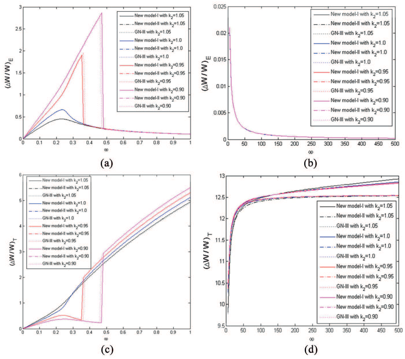
The variation of specific loss, , of an elastic-mode wave for low and high frequencies is shown in Figure 2(a) and (b), respectively. Figure 2(a) shows that there is not much difference in for lower values of under the different models, while each model gives different predictions for specific losses of elastic-mode waves for different values of . The specific loss as under each model and for every value of . This is also clear from the analytical result given by equation (37). Like the phase velocity, for , there are critical frequencies of under all the models and they show corner points in the plots of specific loss of an elastic-mode wave. Figure 2(b) shows that as frequency increases, all models show a negligible difference for variations of . Also as for all values of and under each model, which is in agreement with the analytical result given by equations (33) and (35).
(a) Variation of specific loss of elastic wave () vs. low frequency (). (b) Variation of specific loss of elastic wave () vs. high frequency (). (c) Variation of specific loss of thermal wave () vs. low frequency (). (d) Variation of specific loss of thermal wave () vs. high frequency ().
Figure 2(c) and (d) shows the variation for specific loss, of a thermal-mode wave for low and high values of . Figure 2(c) shows that for very low values of , all different models make similar predictions for specific loss of a thermal wave for a fixed but that as starts increasing, the difference in predictions by different models becomes prominent. As usual, a critical frequency also exists for corresponding to each model for . It is shown by Figure 2(d) that, for higher values of , the difference in is prominent for different values of under all models. Figure 2(d) also shows one very significant observation that, as , approaches under New model I, whereas approaches under New model II and the GN-III model. This fact is in complete agreement with our analytical result, as given by equations (34) and (36).
6.3. Penetration depth
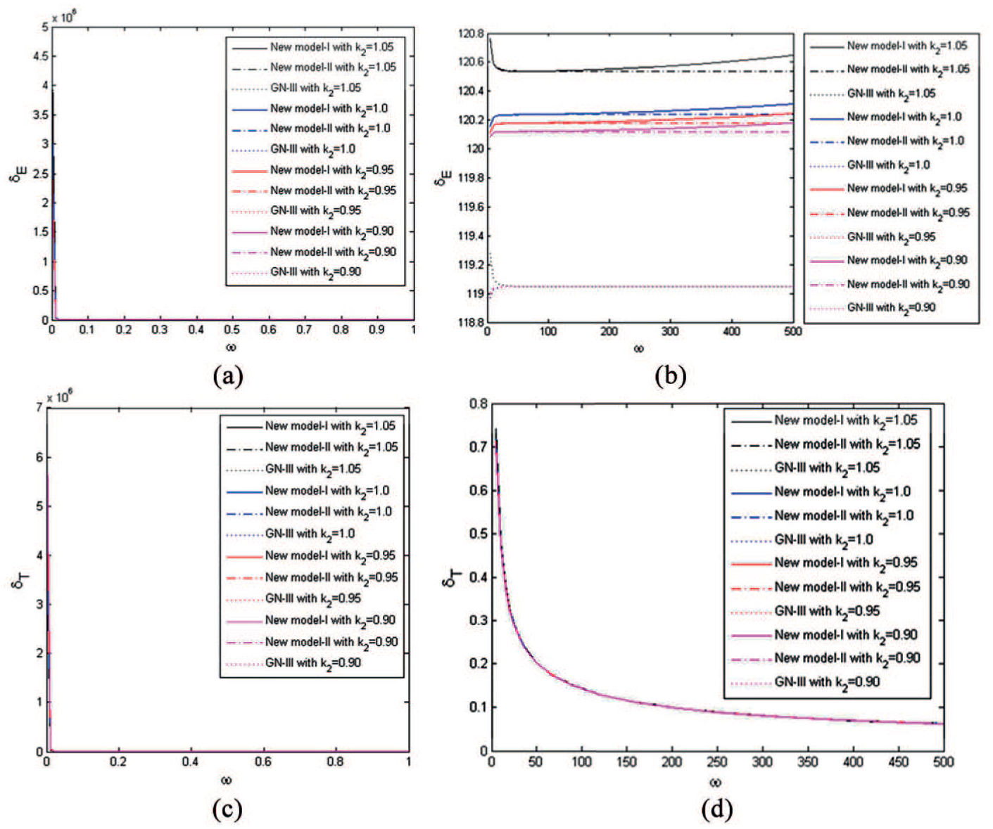
Figure 3(a) and (b) shows the variation for penetration depth of an elastic-mode longitudinal wave for low and high values of . Figure 3(a) shows that there is no difference in under different thermoelasticity theories for a fixed value of , while some difference in for a particular model is present with respect to the variation in . Furthermore, we note that as for each model and for each value of , which is clear from the analytical result given by equation (44). Figure 3(b) shows that for very-high-frequency values, there is a prominent difference in for different models and with respect to as well. Further, from our analytical result (see equation (40)), as well as from numerical results (Figure 3(b)), we get a clear indication that for a fixed , as under New model I. However, in the contexts of New model II and the GN-III model, value (as , which is equal to 120.226 for ) for New model II, which is clear from equation (42) as .
(a) Variation of penetration depth of elastic wave () vs. low frequency (). (b) Variation of penetration depth of elastic wave () vs. high frequency (). (c) Variation of penetration depth of thermal wave () vs. low frequency (). (d) Variation of penetration depth of thermal wave () vs. high frequency ().
Figure 3(c) and (d) shows the variation of penetration depth of a thermal-mode wave under three different thermoelasticity theories for low- and high-frequency values, respectively. Figure 3(c) and (d) shows that there is no prominent difference in for low- as well as high-frequency values with respect to different models and different values of . Further, Figure 3(c) shows that, like the case of , as for each model and for each value of . This is also indicated by the analytical result given by equation (45). Figure 3(b) shows that for New model II and the GN-III model, as . However, New model I predicts that value as , although this limiting value is very close to zero. This is in agreement with analytical results (see equation (41)).
6.4. Amplitude ratio
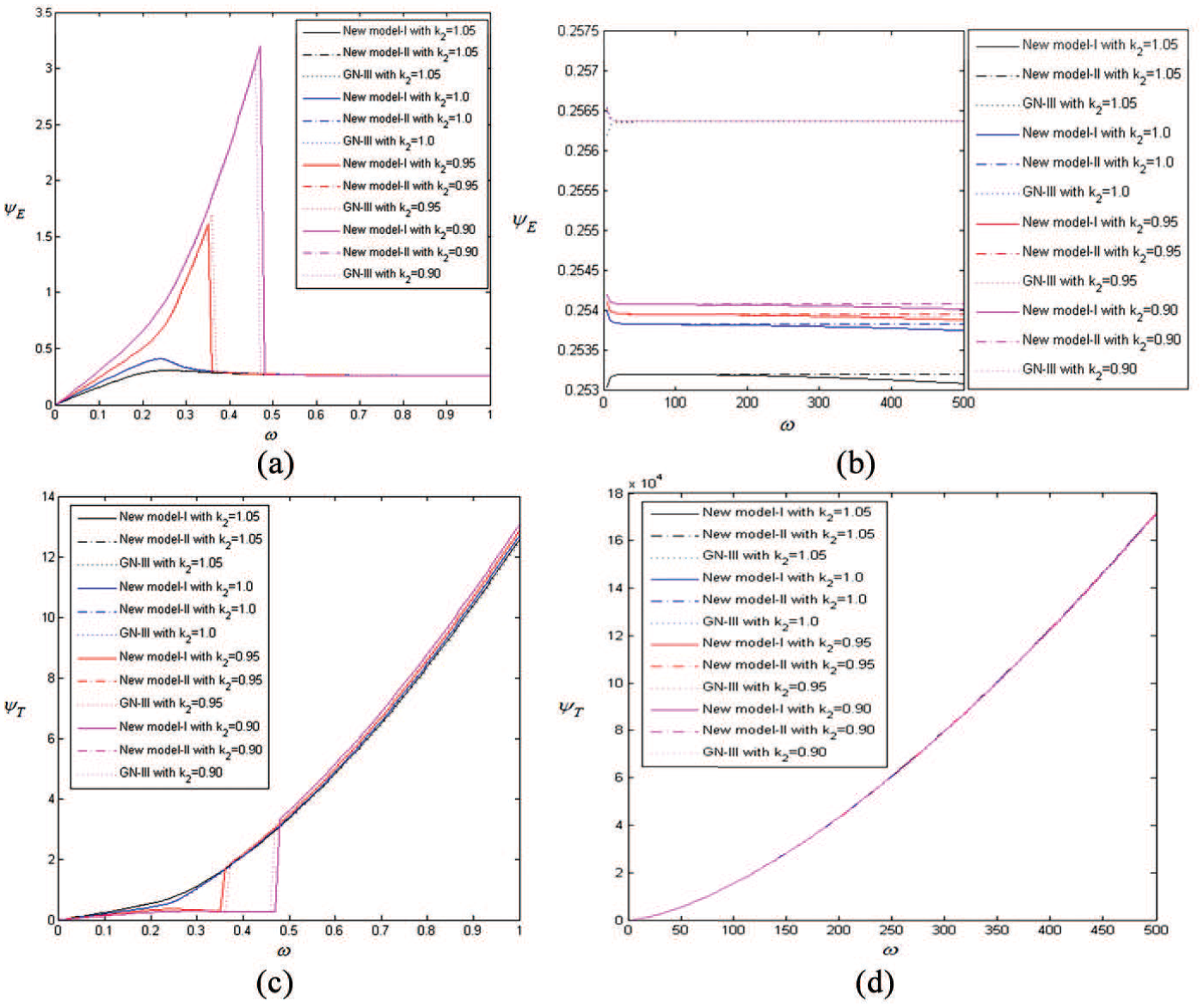
The behavior of amplitude ratio for an elastic-mode longitudinal wave can be observed from Figure 4(a) and (b). From Figure 4(a), we see that there is not much difference in for lower-frequency values. Under all the models as . But for the case when , all the models show some local maximum value before reaching a limiting value. The value of the critical frequency varies with . In Figure 4(b), we observe that for very-high-frequency values, i.e., when , we have (also verified from the analytical result) for New model I, but it decreases toward zero very slowly. In the cases of New model II and the GN-III model, this wave field tends to a constant value. A similar prediction is indicated by the analytic result (see equation (49)) that, for New model II, this value is , which is approximately equal to 0.2548 for . We further note that for different values of this limiting value is different.
(a) Variation of amplitude ratio of elastic wave () vs. low frequency (). (b) Variation of amplitude ratio of elastic wave () vs. high frequency (). (c) Variation of amplitude ratio of thermal wave () vs. low frequency (). (d) Variation of amplitude ratio of thermal wave () vs. high frequency ().
In Figure 4(c), we see that the nature of the amplitude ratio of a thermal-mode wave in the low-frequency case is almost similar in the context of all three models; as in each case. In the case when , we see that under each model, it attains a local minimum value before reaching a limiting value. The position of this critical point varies with the variation of . Figure 4(d) reveals that there is not much difference in the nature of the amplitude ratio of a thermal-mode wave under three models in the high-frequency case. All the models predict that as , which is also verified by our analytical results (see equations (48) and (50)). We do not observe any significant effect of in this case.
7. Conclusions
In this paper, we investigate the behavior of a harmonic plane wave under the very recent heat conduction model with a single delay term introduced by Quintanilla [22]. We consider two types of Taylor series expansion of this new heat conduction model and refer to them as new model I and new model II. Asymptotic results of the dispersion relation solutions for both high- and low-frequency values are presented here for both the models. Moreover, the asymptotic expressions for the important wave components phase velocity, specific loss, penetration depth, and amplitude ratio are derived for both new model I and new model II with variation of frequency and the thermal conductivity rate. We present both analytical and numerical results for a thorough comparison. We show that the analytical results are in perfect match with the numerical results. We further compare our results with the corresponding results of the Green–Naghdi thermoelasticity theory of type III. We observed the following significant facts:
We see that under all the models, only the longitudinal wave is coupled with the thermal field and that there are two different modes of the longitudinal wave. One is elastic and the other is thermal in nature.
For lower-frequency values, we observe from analytical and numerical results that all the models show the same nature for all important wave components. However, for different values of thermal conductivity rate, there is a significant difference in the results under each model. In the case of an elastic wave, each model attains a local maximum and in the case of a thermal wave, it attains a local minimum before tending to a constant limiting value.
For higher-frequency values, there is variation in the nature of New model I and New model II. In this case, New model II is much closer to the GN-III model. There is not much significant change in the nature of each model after taking different values of .
We also observe that the effects of the material constant are more prominent for smaller frequencies and the effects of the term are more significant for higher frequencies.
As , we find that constant under each model, whereas as in all cases.
The theoretical as well as numerical results indicate that, in the case of New model I, the specific loss of the thermal-mode wave is an increasing function of and approaches infinity as . However, this field approaches a constant limiting value under New model II and the GN-III model.
We have and constant as for New model I, whereas constant and in the contexts of the other two models.
As , under New model I and constant under the other two models, whereas under all three models.
New model II and the GN-III model predict similar results that are more similar for high frequency values.
Footnotes
Funding
The author(s) disclosed receipt of the following financial support for the research, authorship, and/or publication of this article: This work was supported by a senior research fellowship (number 2061241025, UGC reference number 17-06/2012(i)EU-V) under University Grant Commission, India.
References
1.
BiotMA. Thermoelasticity and irreversible thermodynamics. J Appl Phys1956; 27: 240–253.
2.
LordHWShulmanY. A generalized dynamical theory of thermoelasticity. J Mech Phys Solids1967; 15: 299–309.
3.
CattaneoC. A form of heat conduction equation which eliminates the paradox of instantaneous propagation. Compt Rend1958; 247: 431–433.
4.
VernotteP. Les paradoxes de la theorie continue de l’equation de la chaleur. Compt Rend1958; 246: 3154–3155.
5.
VernotteP. Some possible complications in the phenomena of thermal conduction. Compt Rend1961; 252: 2190–2191.
GreenAENaghdiPM. A re-examination of the basic postulates of thermomechanics. Proc R Soc Lond A1991; 432: 171–194.
8.
GreenAENaghdiPM. On undamped heat waves in an elastic solid. J Therm Stresses1992; 15: 253–264.
9.
GreenAENaghdiPM. Thermoelasticity without energy dissipation. J Elast1993; 31: 189–209.
10.
TzouDY. The generalized lagging response in small-scale and high-rate heating. Int J Heat Mass Transfer1995; 38(17): 3231–3240.
11.
TzouDY. A unified field approach for heat conduction from macro to micro scales. ASME J Heat Transfer1995; 117: 8–16.
12.
RoychoudhuriSK. On a thermoelastic three-phase-lag model. J Therm Stresses2007; 30: 231–238.
13.
DreherMQuintanillaRRackeR. Ill-posed problems in thermomechanics. Appl Math Lett2009; 22: 1374–1379.
14.
HorganCOQuintanillaR. Spatial behaviour of solutions of the dual-phase-lag heat equation. Math Methods Appl Sci2005; 28: 43–57.
15.
MukhopadhyaySKumarR. Analysis of phase-lag effects on wave propagation in a thick plate under axisymmetric temperature distribution. Acta Mech2010; 210: 331–344.
16.
QuintanillaR. Exponential stability in the dual-phase-lag heat conduction theory. J Non-Eq64 Thermodyn2002; 27: 217–227.
17.
QuintanillaR. A condition on the delay parameters in the one-dimensional dual-phase-lag thermoelastic theory. J Therm Stresses2003; 26: 713–721.
QuintanillaRRackeR. A note on stability of dual-phase-lag heat conduction. Int J Heat Mass Transfer2006; 49: 1209–1213.
20.
QuintanillaRRackeR. Qualitative aspects in dual-phase-lag heat conduction. Proc R Soc Lond A2007; 463: 659–674.
21.
QuintanillaRRackeR. A note on stability in three-phase-lag heat conduction. Int J Heat Mass Transfer2008; 51: 24–29.
22.
QuintanillaR. Some solutions for a family of exact phase-lag heat conduction problems. Mech Res Commun2011; 38: 355–360.
23.
LeseduarteMCQuintanillaR. Phragman–Lindelof alternative for an exact heat conduction equation with delay. Commun Pure Appl Anal2013; 12(3): 1221–1235.
24.
KumariBMukhopadhyayS. Some theorems on linear theory of thermoelasticity for an anisotropic medium under an exact heat conduction model with a delay, Math Mech Solids2017; 22(5): 1177–1189.
25.
QuintanillaR. On uniqueness and stability for a thermoelastic theory. Math Mech Solids2017; 22(6): 1387–1396.
26.
KumarAMukhopadhyayS. An investigation on thermoelastic interactions under an exact heat conduction model with a delay term. J Therm Stresses2016; 39(8): 1002–1016.
27.
LessenM. Motion of thermoelastic solid. Q Appl Math1957; 15: 105–108.
28.
DeresiewiczH. Plane waves in a thermoelastic solid. J Acoust Soc Am1957; 29: 204–209.
29.
ChadwickPSneddonIN. Plane waves in an elastic solid conducting heat. J Mech Phys Solids1958; 6: 223–230.
30.
ChadwickP. Thermoelasticity: The dynamic theory. In: HillRSneddonIN (eds.) Progress in solid mechanics. Amsterdam: North-Holland, 1960; 1: 263–328.
31.
NayfehANemat-NasserS. Thermoelastic waves in solids with thermal relaxation. Acta Mech1971; 12: 53–69.
32.
PuriP. Plane waves in generalized thermoelasticity. Int J Eng Sci1973; 11: 735–744.
33.
AgarwalVK. On plane waves in generalized thermoelasticity. Acta Mech1979; 31: 185–198.
34.
HaddowJBWegnerJL. Plane harmonic waves for three thermoelastic theories. Math Mech Solids1996; 1: 111–127.
35.
ChandrasekharaiahDS. Thermoelastic plane waves without energy dissipation. Mech Res Commun1996; 23: 549–555.
36.
PrasadRKumarRMukhopadhyayS. Propagation of harmonic plane waves under thermoelasticity with dual-phase-lags. Int J Eng Sci2010; 48: 2028–2043.
37.
PuriPJordanPM. On the propagation of plane waves in type-III thermoelastic media. Proc R Soc Lond A2004; 460: 3203–3221.
38.
KothariSMukhopadhyayS. Study of harmonic plane waves in rotating thermoelastic media of type III. Math Mech Solids2012; 17(8): 824–839.
39.
PonnusamyS. Foundation of complex analysis. New Delhi: Narosa Publishing House, 2005.