1. Geometrical preliminaries
For details about the classical notions of differential geometry recalled in this section, see, e.g. Ciarlet [1, 2].
Greek indices, except
and
, take their values in the set
, while Latin indices, except when they are used for indexing sequences, take their values in the set
, and the summation convention with respect to repeated indices is systematically used in conjunction with these two rules. The notation
designates the three-dimensional Euclidean space; the Euclidean inner product and the vector product of
are denoted
and
; the Euclidean norm of
is denoted
. The notation
designates the Kronecker symbol.
Given an open subset
of
, notations such as
,
or
,
, designate the usual Lebesgue and Sobolev spaces, and the notation
designates the space of all functions that are infinitely differentiable over
and have compact supports in
. The notation
designates the norm in a normed vector space X. Spaces of vector-valued functions are denoted with boldface letters. The notation
designates the norm of the Lebesgue space
, and the notation
, designates the norm of the Sobolev space
,
.
A domain in
is a bounded and connected open subset
of
, whose boundary
is Lipschitz-continuous, the set
being locally on a single side of
.
Let
be a domain in
, let
denote a generic point in
and let
and
. A mapping
is an immersion if the two vectors

are linearly independent at each point
. Then the image
of the set
under the mapping
is a surface in
, equipped with
as its curvilinear coordinates. Given any point
, the vectors
span the tangent plane to the surface
at the point
, the unit vector

is normal to
at
, the three vectors
form the covariant basis at
and the three vectors
defined by the relations

form the contravariant basis at
; note that the vectors
also span the tangent plane to
at
and that
.
The first fundamental form of the surface
is defined by means of its covariant components

or by means of its contravariant components

Note that the symmetric matrix field
is the inverse of the matrix field
, that
and
, and that the area element along
is given at each point
, by
, where

Given an immersion
, the second fundamental form of the surface
is defined by means of its covariant components

or by means of its mixed components

and the Christoffel symbols associated with the immersion
are defined by

The Gaussian curvature at each point
, of the surface
is defined by

(the denominator in this relation does not vanish, since
is assumed to be an immersion). Note that the Gaussian curvature
at the point
is also equal to the product of the two principal curvatures at this point.
A surface
defined by means of an immersion
is said to be elliptic if its Gaussian curvature is everywhere
in
or, equivalently, if there exists a constant
such that

Given an immersion
and a vector field
, the vector field

can be viewed as a displacement field of the surface
, and is thus defined by means of its covariant components
over the vectors
of the contravariant bases along the surface. If the norms
are small enough, the mapping
is also an immersion, so that the set
is also a surface in
, equipped with the same curvilinear coordinates as those of the surface
, called the deformed surface corresponding to the displacement field
. One can then define the first fundamental form of the deformed surface by means of its covariant components

and the second fundamental form of the deformed surface by means of its covariant components

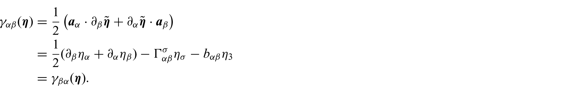
The linear part with respect to
in the difference

is called the linearized change of metric, or strain, tensor associated with the displacement field
, the covariant components of which are then given by
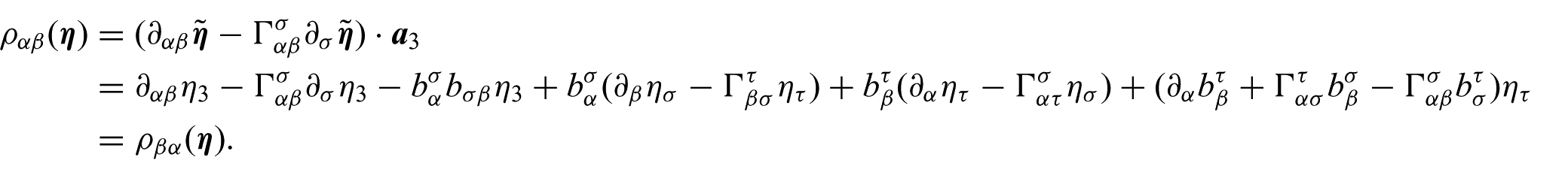
The linear part with respect to
in the difference

is called the linearized change of curvature tensor associated with the displacement field
, the covariant components of which are then given by
2. A natural Koiter’s model for a general shell subject to a confinement condition
Let
be a domain in
with boundary
, and let
be a non-empty relatively open subset of
. For each
, we define the sets

we let
designate a generic point in the set
, and we let
. Hence, we also have
and
. The set
is thus a subset of the lateral face of the undeformed reference configuration.
In all that follows, we are given an injective immersion
and
, and we consider a shell with middle surface
and with constant thickness
. This means that the reference configuration of the shell is the set
, where the mapping
is defined by

Note that the injectivity assumption is made here for physical reasons, but that it is otherwise not needed in the proofs. One can then show (compare with Theorem 3.1-1 of Ciarlet [1] or Theorem 4.1-1 of Ciarlet [2]) that, if the thickness
is small enough, such a mapping
is a
–diffeomorphism from
onto
, and hence is in particular an injective immersion, in the sense that the three vectors

are linearly independent at each point
; these vectors then constitute the covariant basis at the point
, while the three vectors
, defined by the relations

constitute the contravariant basis at the same point.
It will be implicitly assumed in what follows that the immersion
is injective and that
is small enough so that
is a
-diffeomorphism onto its image.
We henceforth assume that the shell is made of a homogeneous and isotropic linearly elastic material and that its reference configuration
is a natural state, i.e., is stress-free. As a result of these assumptions, the elastic behaviour of this elastic material is completely characterized by its two Lamé constants
and
(see, e.g., Section 3.8 in Ciarlet [3]).
We also assume that the shell is subjected to applied body forces whose density per unit volume is defined by means of its contravariant components
, i.e., over the vectors
of the covariant bases, and to a homogeneous boundary condition of place along the portion
of its lateral face, i.e., the admissible displacement fields vanish on
.
A commonly used two-dimensional set of equations for modelling such a shell (‘two-dimensional’ in the sense that it is posed over
instead of
) was proposed in 1970 by Koiter [4, 5]. We now describe the modern formulation of this model.
First, define the space

where the symbol
denotes the outer unit normal derivative operator along
, and define the norm
by

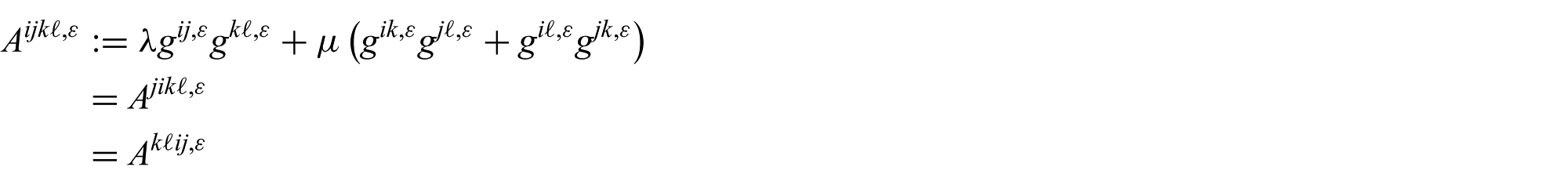
Next, define the fourth-order two-dimensional elasticity tensor of the shell, viewed here as a two-dimensional linearly elastic body, by means of its contravariant components

Finally, define the bilinear forms
and
by
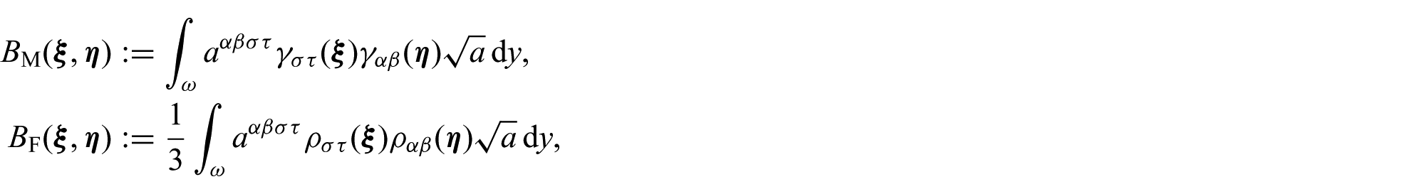
for each
and each
, and define the linear form
by

where
at each
.
Then the total energy of the shell is the quadratic functional
defined by

The terms
and
respectively represent the membrane part and the flexural part of the total energy, as aptly recalled by the subscripts ‘M’ and ‘F’.
In Koiter’s model, the unknown ‘two-dimensional’ displacement field
of the middle surface
of the shell is such that the vector field
should be the solution of the following problem: find a vector field
that satisfies

or equivalently, find
that satisfies the following variational equations:

As first shown by Bernadou and Ciarlet [6] (see also Bernadou et al. [7]), this problem has one and only one solution.
Assume now that the shell is subject to the following confinement condition: the unknown displacement field
of the middle surface of the shell must be such that the corresponding ‘deformed’ middle surface remains in a given half-space, of the form

where
is a given non-zero vector. Equivalently, the deformed middle surface must remain ‘on one side’ of the plane
, then viewed as an obstacle; it is this observation that motivates the use of the term ‘obstacle problem’ in the title of this paper. Of course, it will be henceforth assumed that the ‘undeformed’ middle surface satisfies this confinement condition, i.e., that

It is thus physically sound to assume that, while the total energy of the shell remains unchanged, the set over which the energy is to be minimized is now a strict subset of
(denoted
in the following) that takes into account the imposed confinement condition. These assumptions lead to the following definition of a problem, denoted
in the next theorem, which constitutes Koiter’s model for a shell subject to a confinement condition. In what follows, ‘a.e.’ stands for ‘almost everywhere’.
Theorem 1. The minimization problem: Find

such that

has one and only one solution.
Besides, this solution is also the unique solution of problem
: find
that satisfies the following variational inequalities:

Proof. The bilinear forms
and
and the linear form
are clearly continuous. Since the two-dimensional elasticity tensor
of the shell is uniformly positive definite, in the sense that there exists a constant
such that

for all
and all symmetric matrices
, the bilinear form

is
-elliptic, on the one hand, thanks to the Korn’s inequality on a general surface due to [6] (see also [7]; this inequality is also recalled in Theorem 5 below; note that this inequality holds in particular because
-meas
).
On the other hand, it is easily seen that
is a non-empty (by assumption), closed (any convergent sequence in
contains a subsequence that pointwise converges to the same limit), and convex, subset of the space
.
Hence, by a classical result (see, e.g., Duvaut and Lions [8], Glowinski [9], or Theorems 6.1–1 and 6.1–2 of Ciarlet [10]), this minimization problem, or equivalently problem
, has one and only one solution. □
Problem
is meant to apply to any shell, i.e., regardless of the subset
of
, the asymptotic behaviour of the applied forces as
, and the geometry of the middle surface. It is in this sense that it is a model for a ‘general’ shell.
Conversely, it has been shown (in the series of papers by Ciarlet and Lods [11, 12], and Ciarlet et al. [13]; see also Chapters 4, 5 and 6 in Ciarlet [1]) that a rigorous asymptotic analysis of the equations of ‘unconstrained’ (i.e., not subject to any confinement condition) linearly elastic shells as their thickness approaches zero leads one to distinguish three types of ‘limit’ equations, corresponding to elliptic membrane shells, generalized membrane shells and flexural shells, depending on the subset
, the behaviour of the applied forces as
and the geometry of the middle surface. It has been furthermore shown (see Theorems 3.2, 4.1 and 5.2 in the references provided just before) that, remarkably, the equations of the linear two-dimensional ‘unconstrained’ Koiter’s model (i.e., that described at the beginning of this section) exhibit exactly the same ‘limit’ behaviour, thus fully justifying Koiter’s model in the ‘unconstrained’ case, i.e., when no confinement condition is imposed.
It is thus natural to investigate whether our proposed Koiter’s model for a shell subject to a confinement condition shares the same features. This is the primary objective of this paper.
To this end, we thus need to identify the possible limit behaviours of the solution to our model, i.e., of problem
, as
, depending on the type of shell under consideration: this is the objective of the next three sections.
3. Koiter’s model for an elliptic membrane shell subject to a confinement condition
Consider a linearly elastic shell, subject to the various assumptions set forth in Section 2. Following the terminology proposed in Section 4.1 of Ciarlet [1], such a shell is said to be a linearly elastic elliptic membrane shell if the following two additional assumptions are satisfied: first,
, i.e., the homogeneous boundary condition of place is imposed over the entire lateral face
of the shell, and second, its middle surface
is elliptic, according to the definition given in Section 1. Note that the assumption
implies that the space
introduced in Section 2 now reduces to

To begin with, we recall a crucial inequality that holds for elliptic surfaces.
Theorem 2. Let
be a domain in
and let
be an immersion such that
is an elliptic surface. Define the space

and the norm
by

Then there exists a constant
such that

for all
.
This inequality, which was proves by Ciarlet and Lods [14] and Ciarlet and Sanchez-Palencia [15] (see also Ciarlet [1], Theorems 2.7–3), constitutes an example of a Korn inequality on an elliptic surface; it constitutes a ‘Korn inequality’ in the sense that it provides an estimate of an appropriate norm of a displacement field defined on an elliptic surface in terms of an appropriate norm of a specific ‘measure of strain’ (here, the linearized change of metric tensor) corresponding to the displacement field considered.
The forthcoming analysis resorts to an argument similar to the one in Theorem 7.2-1 (itself based on Destuynder [16], Sanchez-Palencia [17], Caillerie and Sanchez-Palencia [18] and, especially, on Theorem 2.1 in Ciarlet and Lods [19]) of Ciarlet [1], and constitutes the first convergence result of this paper. The set
appearing in the next theorem is defined in Theorem 1.
Theorem 3. Let
be a domain in
and let
be an immersion. Consider a family of elliptic membrane shells with thickness
approaching zero and with each having the same middle surface
, and assume that there exist functions
independent of
such that

Finally, assume that the following ‘density property’ holds:

For each
, let
denote the solution to problem
(Theorem 1). Then the following convergences hold:

where
is the unique solution to the following problem
: Find

that satisfies the following variational inequalities:

where

Proof. (i) Problem
has one and only one solution. To see this, we notice that the bilinear form defined by

is continuous and
-elliptic thanks to the Korn’s inequality of Theorem 2, the set
is a non-empty closed and convex subset of
, and the linear form
defined by

is continuous over
.
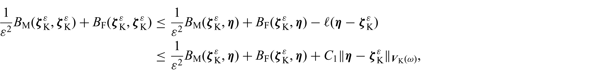
(ii) Uniform boundedness of the family
. In what follows, strong and weak convergences are respectively denoted → and ⇀. By virtue of the assumption made on the applied body force density, the variational inequalities in problem
reduce to

for all
; hence,

for all
. Thanks to the uniform positive definiteness of the tensor
and to Theorem 2, there exists a constant
such that

Besides, the continuity of the bilinear forms
and
and the continuity of the linear form
imply that there exists a constant
such that

Letting
thus gives

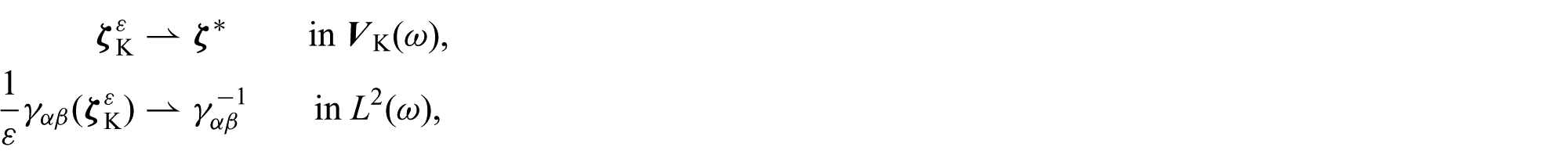
(iii) Weak convergence of the family
. By (ii), the family
is bounded in
. Therefore, there exists a subsequence, still denoted
, a vector field
and functions
such that:

the second convergence being also a consequence of the uniform positive definiteness of the tensor
. Then
, since the set
is non-empty, closed and convex (compare with, e.g., Theorem 3.7 in Brezis [20] or Theorem 5.13–1 in Ciarlet [10]). Fix
and observe that, since the vector field
solves problem
, the following variational inequalities hold:

so that letting
gives

on the one hand. On the other hand,

which in turn implies that

Hence, letting
gives

In conclusion,

Furthermore, the assumed ‘density property’ gives

which shows that
is a solution to problem
. Since problem
admits a unique solution, we conclude that
. Hence, the whole family
weakly converges to
in
as
.
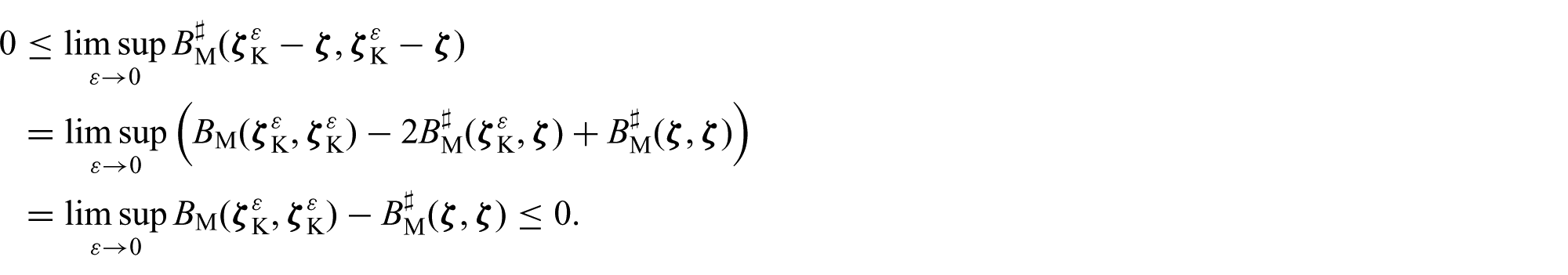
(iv) Strong convergence of the family
. The
-ellipticity of the bilinear form
and the assumed ‘density property’ together give
for all
. Hence, letting
and letting
gives

which shows that

as was to be proved. □
Note that realistic sufficient conditions insuring that the ‘density property’ holds are given by Ciarlet et al. Ciarlet et al. [21] (see also Ciarlet et al. [22]).
4. Koiter’s model for a generalized membrane of the ‘first kind’ subjectto a confinement condition
Consider a linearly elastic shell subject to the various assumptions set forth in Section 2. Following the terminology proposed in Section 5.1 of Ciarlet [1], such a shell is said to be a linearly elastic generalized membrane shell if the following two additional assumptions are simultaneously satisfied. First,
(an assumption that is satisfied if
is a non-empty relatively open subset of
, as assumed here). Second, the space of admissible linearized inextensional displacements defined by

does not contain any non-zero vectors, i.e.,

but the shell is not an elliptic membrane shell in the sense of Section 3 (note in this respect that, indeed, the space
also reduces to
if the shell is an elliptic membrane one; compare with Theorem 2). The second condition in the definition of a generalized membrane shell, namely

is equivalent to stating that the semi-norm
defined by

for each
becomes a norm over the space

Generalized membranes are themselves subdivided into two categories described in terms of the spaces

A generalized membrane shell is ‘of the first kind’ if

or, equivalently, if the semi-norm
is already a norm over the space
(hence, a fortiori, over the space
).
Otherwise, i.e., if

or, equivalently, if the semi-norm
is a norm over
but not over
, the linearly elastic shell is a generalized membrane shell ‘of the second kind’. In this paper, we shall only consider generalized membranes of the ‘first kind’ (which are most frequently encountered in practice).
The forthcoming analysis resorts to an argument similar to that of Caillerie and Sanchez-Palencia [18] used in Theorem 7.2–2 of Ciarlet [1] (itself based on Caillerie and Sanchez-Palencia [18] and, especially, on Ciarlet and Lods [12]) and constitutes the second convergence result of this paper.
In addition to a simple assumption regarding the asymptotic behaviour of the applied forces (in effect, the same as for elliptic membrane shells; compare with Theorem 3), we will need (as in the previous references) to assume that the applied body forces are admissible, in the sense that there exist functions
independent of
such that, for each
, the linear form
appearing in problem
can also be written as

Note that this assumption is stronger than the assumption that there exist functions
independent of
such that

made for elliptic membrane shells, since it implies that the linear forms
are now continuous with respect to
.
Theorem 4. Let
be a domain in
and let
be an immersion. Consider a family of generalized membrane shells ‘of the first kind’ with thickness
approaching zero and with each having the same middle surface
, and assume that each shell is subject to a boundary condition of place along a portion of its lateral face, whose middle curve is the set
. Define the spaces

For each
, let
denote the solution to problem
(Theorem 1). Then the following convergence holds:

where
denotes the unique solution to problem
. Find

that satisfies the following variational inequalities:

where
and
designate the unique continuous linear extensions from
to
of the bilinear form
, and of the linear form
defined by

Proof. (i) Problem
has one and only one solution. We first observe that the space
is also the completion of the space
with respect to the norm
. Clearly, problem
admits a unique solution, since the bilinear form
is continuous and
-elliptic (recall that the tensor
is uniformly positive definite), the set
is non-empty, closed with respect to
, and convex, and the linear form
is continuous.
(ii) Uniform boundedness of the family
. Because the applied body forces are admissible, the variational inequalities appearing in the problem
read

for all
. By virtue of the continuity of the linear form
with respect to the norm
, there then exists a constant
such that

for all
. Thanks to the uniform positive definiteness of the tensor
, there exists a constant
such that

Hence, letting
gives

This inequality shows that the family
is bounded in
and that each family
is bounded in
.
(iii) Weak convergence of the family
. As a consequence of (ii), there exist a subsequence, still denoted
, a vector field
and functions
, such that

The vector field
belongs to the set
, which is a non-empty, closed and convex subset of
.
Letting
in these variational inequalities gives

and, therefore, by definition of
,

on the one hand. On the other hand, we have

which in turn implies

Therefore,

which shows that
is a solution to problem
. Since the solution to problem
is unique by (i), we conclude that

and that the whole family
weakly converges to
in
as
.
(iv) Strong convergence of the family
. The positive definiteness of the two-dimensional fourth-order elasticity tensor of the shell, together with the definition of the norm
and of the bilinear form
and its extension
, show that establishing the announced strong convergence is equivalent to establishing the convergence

Since
, we have, in particular,

Noting that

and noting that the weak convergence
in
as
, established in (iii), implies that

we infer from these relations that
Hence, the strong convergence

holds, as announced. □
5. Koiter’s model for a flexural shell subjected to a confinement condition
Consider a linearly elastic shell, subject to the various assumptions set forth in Section 2. Following the terminology proposed in Section 6.1 of Ciarlet [1], such a shell is said to be a linearly elastic flexural shell if the following two additional assumptions are satisfied: first,
(an assumption that is satisfied if
is a non-empty relatively open subset of
, as here), and second, the following space of admissible linearized inextensional displacements:

contains non-zero functions, i.e.,

To begin with, we state a crucial inequality that holds for ‘general’ surfaces (this inequality was already needed in the proof of Theorem 1).
Theorem 5. Let
be a domain in
and let
be an immersion. Let
be a non-empty relatively open subset of
. Define the space

Then there exists a constant
such that
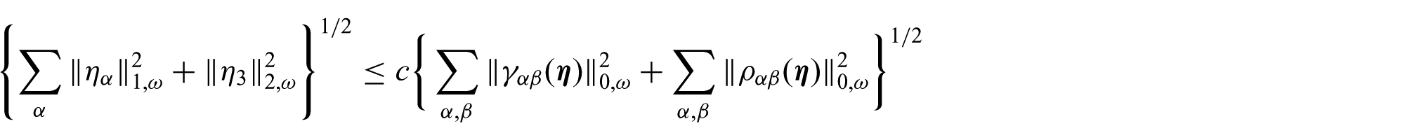
for all
.
This inequality, was first proved by Bernadou and Ciarlet [6] (see also Bernadou, Ciarlet and Miara [7] and Ciarlet [1], Theorems 2.7–3), constitutes an example of a Korn inequality on a general surface; it constitutes a ‘Korn inequality’ in the sense that it provides a basic estimate of an appropriate norm of a displacement field defined on a surface in terms of an appropriate norm of a specific ‘measure of strain’ (here, the linearized change of metric tensor and the linearized change of curvature tensor) corresponding to the displacement field considered.
The forthcoming analysis resorts to an argument similar to the one used in Theorem 7. 2–3 of Ciarlet [1] (itself based on Sanchez- Palencia [21] and, especially, on Ciarlet and Lods [17]) and constitutes the third convergence result of this paper.
Theorem 6. Let
be a domain in
and let
be an immersion. Consider a family of flexural shells with thickness
approaching zero and with each having the same middle surface
. Let
be a non-empty relatively open subset of
, and assume that each shell is subject to a boundary condition of place along a portion of its lateral face, whose middle curve is the set
. Finally, assume that there exist functions
independent of
such that:

For each
, let
denote the solution to problem
(Theorem 1). Then the following convergence holds:

where
denotes the solution to problem
: Find

that satisfies the following variational inequality:

where

Proof. (i) Problem
admits a unique solution. To see this, observe that the bilinear form
, which is defined by

is continuous and
-elliptic,
is a non-empty closed and convex subset of
, and the linear form
defined by

is continuous over
. Hence the conclusion follows.
(ii) Uniform boundedness of the family
. By virtue of the assumption on the applied body forces, the variational inequalities in problem
read

for all
, and by the continuity of the linear form
, there exists a constant
such that
for all
. Thanks to the uniform positive definiteness of the tensor
and Theorem 5, there exists a constant
such that

Hence, combining these two inequalities and letting
gives

(iii) Weak convergence of the family
. By (ii), the family
is bounded in
. Therefore, there exists a subfamily, still denoted
, a vector field
and functions
, such that
the second weak convergence being a consequence of the uniform positive definiteness of the tensor
. The same weak convergence in turn implies that

on the one hand. On the other hand, the weak convergence
in
clearly implies that

Hence, the uniqueness of the weak limit shows that

i.e., that
. Besides,
belongs to
, because
is a non-empty, closed and convex subset of
. In conclusion,
belongs to
.
For any given
, the following inequality holds:
so that, letting
in this inequality, we obtain

We also have

which in turn implies that

Hence, letting
, we obtain

Therefore,

We have thus shown that

i.e., that
is a solution to problem
. Since problem
admits a unique solution, we conclude that
. Hence, the whole family
weakly converges to
in
as
.
(iv) Strong convergence of the family
. Combining the Korn’s inequality on a general surface (Theorem 5), the strong convergence
in
and the uniform positive definiteness of the tensor
, establishing the strong convergence
in
amounts to establishing that
as
.
Noting that we have
since
, we obtain

Hence,

which completes the proof. □
6. Justification of the proposed model
Given an immersion
and
small enough, let the sets
,
, the
–diffeomorphism
and the vector fields
and
be defined as in Section 2.
One then defines the metric tensor by means of its covariant components

or by means of its contravariant components

Note that the symmetric matrix field
is then the inverse of the matrix field
, that
and
and that the volume element in
is given at each point
,
, by
, where

One also defines the Christoffel symbols associated with the immersion
by

Given a vector field
, the associated vector field

may be viewed as a displacement field of the reference configuration
of the shell, thus defined by means of its covariant components
over the vectors
of the contravariant bases in the reference configuration.
If the norms
are small enough, the mapping
is also an immersion, so that one can also define the metric tensor of the deformed configuration
by means of its covariant components

The linear part with respect to
in the difference
is then called the linearized strain tensor associated with the displacement field
, the covariant components of which are then given by
The functions
are called the linearized strains in curvilinear coordinates associated with the displacement field
.
As in Sections 2 to 5, we assume that, for each
, the reference configuration
of the shell is in its natural state (i.e., it is ‘stress-free’) and that the material constituting the shell is homogeneous, isotropic and linearly elastic, the behaviour of which is thus governed by its two Lamé constants
and
.
We then consider a specific obstacle problem for such a shell, in the sense that the shell is subject to a confinement condition, expressing that any admissible displacement vector field
must be such that the corresponding deformed configuration remains in the same half-space as in Section 2, i.e., of the form

where
is a non-zero vector given once and for all. In other words, every admissible displacement field must satisfy the ‘constraint’

or possibly only almost everywhere in
. Note that, unlike the obstacle-free case, we do not consider applied surface forces.
We will, of course, assume that the reference configuration satisfies the confinement condition, i.e., that

It is worth pointing out that this confinement condition considerably departs from the usual Signorini condition preferred by most authors, who usually require that only the points of the undeformed and deformed ‘lower face’
of the reference configuration satisfy the confinement condition (see, e.g., Léger and Miara [23–25] or Rodrguez-Ars [26]). The confinement condition considered in this investigation is more physically realistic, since a Signorini condition imposed only on the lower face of the reference configuration does not prevent – at least theoretically – other points of the deformed reference configuration from ‘crossing’ the plane
and then ending up on the ‘other side’ of this plane.
The mathematical modelling of such an obstacle problem for a linearly elastic shell is then clear; since, apart from the confinement condition, the rest, i.e., the function space and the expression of the quadratic total energy
, is classical. More specifically, let
denote the contravariant components of the three-dimensional elasticity tensor of the shell, viewed here as a three-dimensional elastic body. Then the unknown of the problem, which is the vector field
, where the functions
are the three covariant components of the unknown ‘three-dimensional’ displacement vector field
of the reference configuration of the shell, should minimize the energy
defined by

for each
over the set of admissible displacements defined as follows:

The solution to this minimization problem exists and is unique; it can also be characterized as the unique solution of a set of appropriate variational inequalities, as shown in the next theorem.
Theorem 7 The quadratic minimization problem: Find a vector field
such that

has one and only one solution, which is also the unique solution of the variational problem
: Find

that satisfies the following variational inequalities:

for all
.
Proof. Define the space

Then, thanks to the uniform positive definiteness of the elasticity tensor
and to the boundary condition of the place satisfied on
(recall that
is a non-empty, relatively open, subset of
), it can be shown (see Ciarlet [2], Theorems 3.8–3 and 3.9–1) that the continuous and symmetric bilinear form

is
-elliptic; moreover, the linear form

is clearly continuous. Finally, the set
is non-empty (by assumption), closed in
(any convergent sequence in
contains a subsequence that pointwise converges almost everywhere to its limit) and convex (as is immediately verified).
The existence and uniqueness of the solution to the minimization problem and its characterization by means of variational inequalities is then a consequence of the projection theorem. □
We now recall the convergence result recently established by Ciarlet et al. [21] (see also Ciarlet et al. [22]) regarding the asymptotic behaviour as
of the solution to problem
when the shell is an elliptic membrane one.
Theorem 8. Let
be a domain in
and let
be an immersion. Consider a family of elliptic membrane shells with thickness
approaching zero and with each having the same middle surface
and assume that there exist functions
independent of
such that the following assumption on the applied body force density holds:

Finally, assume that the following ‘density property’ holds:

Let
denote the solution to problem
(Theorem 3) and, for each
, let
denote the solution to problem
(Theorem 1). Then the following convergences hold:
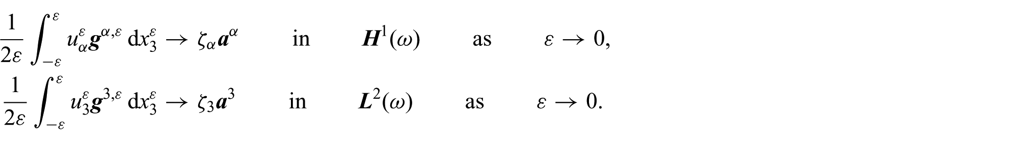
A comparison with the convergences

established in Theorem 3 thus shows that the solution to the three-dimensional obstacle problem
and to the two-dimensional obstacle problem
exhibit the same limit behaviour as
. This observation then fully justifies the formulation of our proposed Koiter’s model for an elliptic membrane shell subjected to a confinement condition.
Similar justifications of our proposed Koiter’s model for a generalized membrane shell or for a flexural shell subjected to a confinement condition will be provided in forthcoming works.
