Transient interior analytical solutions of Lamb’s problem

Abstract

The classical three-dimensional Lamb’s problem is considered for an inclined surface point load of Heaviside time dependence. Attention is focused upon the acquisition of the transient elastodynamic analytical solutions for interior points through a unified method of analysis that is valid for arbitrary Lamé constants. The method of elastodynamic potentials is employed jointly with integral transforms to treat the corresponding initial boundary value problem. To derive the time-domain solutions, some integral equations are encountered, the solutions of which are found via a modified version of the Cagniard–Pekeris method. The final solutions are obtained as finite integrals that are amenable to numerical calculations. They are also expressed in the form of Green’s functions. The limit case of infinite time is investigated analytically to derive the closed-form expressions for the limits of the solutions as the temporal variable tends to infinity. As expected, the results are found to be equivalent to Boussinesq–Cerruti solutions in elastostatics. The elastodynamic solutions are also evaluated numerically to plot several time-history diagrams, depicting the transient motions of the interior points, especially of the points close to the boundary so as to illustrate the formation of forced Rayleigh waves at shallow depths within the elastic half-space.

Keywords

Lamb’s problem transient wave motions interior solutions integral equations Cagniard–Pekeris method elastic half-space

1. Introduction

The analytical study of motions within elastic solids has been of immense theoretical and practical interest from the early days of the development of the mathematical theory of elasticity [1]. Of greater significance, and inevitably of much more mathematical complexity, in this context are the investigations concerned with the propagation of transient waves in solids, as compared to the studies of monochromatic wave motions. One of the first contributions in this category might be the solutions presented by Stokes in 1849 for the emission of waves in an unbounded homogeneous, isotropic, linear elastic medium due to an interior point load with arbitrary time dependence (refer to, e.g. [1,2]). In the ensuing decades, Rayleigh discovered a new type of wave that propagated along and remained confined to the vicinity of the free surface of an elastic half-space [3]. After Rayleigh, Lamb set out to investigate a number of problems related to the forced surface motions of elastic media [4]. Starting from the easier two-dimensional problems, generalising and developing his analyses to the problems in three dimensions, Lamb delineated a certain class of problems that gave directions for many later researches. The most important of those problems, often referred to as the three-dimensional Lamb’s problem in the literature, investigates the surface motions of an elastic half-space due to a surface point excitation [2, 5]. Lamb’s line of attack in his memoir was treating the problem first in the case of a simple-harmonic excitation and then generalising the solutions thereof to the case of an arbitrary impulsive excitation via Fourier synthesis [4]. In this manner, he derived surface solutions for a vertical surface point load in the form of double integrals, and investigated the influences of various wavefronts (body and surface waves) upon the character of surface motions. Lamb’s problem and its various extensions or special cases have been the subject of many further researches by others. For instance, the simpler two-dimensional case of Lamb’s problem for propagation of cylindrical wavefronts was treated by Lapwood [6].

Pekeris was the first researcher to obtain exact, closed-form surface solutions and time-history diagrams for the case of a vertical surface point load with Heaviside time dependence and for the particular case of equal Lamé constants, i.e. $λ = μ$ (or, equivalently, Poisson’s ratio equal to 0.25) [7]. The restriction of Poisson’s ratio in Pekeris’ work was removed much later by Mooney [8]. Pekeris also investigated the same problem for the case in which the load was buried at a finite depth within the medium [9], and found surface solutions in the form of integrals that were later evaluated numerically [10]. Pekeris’ method of solution was different from Lamb’s in the sense that he used the notions of Heaviside’s operational calculus, instead of the classical method of Fourier superposition. In the course of this method, utilisation of the Cagniard’s complex-analytic techniques [11] becomes natural and necessary in order to interpret the operational solutions in the time-domain. Chao [12] extended the work of Pekeris for the case of a horizontal surface point load and he used the equivalent, yet more rigorous, methods of modern operational calculus (i.e. the use of Laplace transforms [13]). Chao also gave the solutions for the points inside the medium but directly under the point of application of the load [12].

Although it might not have been a severe restriction, the Pekeris-Chao solutions and time-history diagrams were only presented for the special case $λ = μ$ . This restriction was removed later by Kausel, who presented the closed-form surface solutions due to vertical or horizontal surface point loads as well as dipoles, in their simplest and most elegant form, for solids with arbitrary material constants [14]. Accordingly, Kausel’s paper [14] may be regarded as the concluding account to surface solutions of Lamb’s problem for vertical or horizontal surface point loads of Heaviside time dependence. Results equivalent to the ones found by Kausel [14] can also be found in a much earlier paper by Richards [15], which studied three-dimensional crack propagation. However, Richards [15] only presented the final solutions without giving their derivation, which is in fact rather complicated.

The acquisition of interior solutions (solutions for points inside the half-space), however, has seen much slower a progress, owing chiefly to the fact of mathematical complexities. Eason used the joint Hankel-Laplace integral transforms for Lamb’s problem for surface disc or point load excitations [16]. Direct inversion of the Laplace transform via some complicated contour integrations along branch cuts in the complex plane of Laplace transform parameter led Eason to derive the interior solutions for vertical surface loads in the form of finite integrals. He evaluated his point load solutions numerically and plotted them, yet solely for the case of large time, after the arrival of transverse waves [16].

Gakenheimer and Miklowitz, considered an interesting generalisation of Lamb’s problem where a vertical point load suddenly applied onto the surface of an elastic half-space began moving with constant speed along a straight line on that surface [17]. Using the Cagniard–de Hoop method (i.e. Cagniard’s method with de Hoop’s modifications [18]), these two authors studied interior solutions arising from different load speeds. The important special case of zero load speed is, indeed, Lamb’s problem for a suddenly applied vertical point load. For this particular case and by fixing $λ = μ$ , Gakenheimer evaluated the integral solutions numerically in a subsequent paper [19] and plotted time-histories that extended the work of Eason [16]. Bakker et al. [20] later revisited Gakenheimer’s travelling point load problem for which they have given a much more detailed analysis by going into the details of the solution method. This aspect had been previously missing in both references [17] and [19].

Another important contribution to Lamb’s problem is the work of Johnson [21], in which the problem was treated for an interior point force. This can also be considered as a generalisation of Pekeris’ buried pulse problem [9], for which the excitation is no longer restricted to be a vertical point load, but can be horizontal as well. Johnson’s account [21] is based upon the use of bilateral Laplace transforms on the spatial variables (in the Cartesian coordinate system) and the unilateral Laplace transform on the temporal variable. Then, utilising the Cagniard–de Hoop method, he presented integral expressions for the solutions as well as their spatial derivatives, at the interior and boundary points of the half-space. Indeed, Johnson’s boundary solutions (solutions on the free surface) are reciprocal to the interior solutions found in the current paper. However, the inversion of integral transforms is not discussed in Johnson’s paper [21], but only briefly outlined; although, the inversion process is not trivial in this subject. In contrast to Johnson’s research, in the present paper the problem is elegantly formulated and solved in a cylindrical coordinate system ab initio. This leads to a certain class of integral equations, which are not only intrinsically interesting, but can also be utilised for further development of the theory. The detailed analysis of the mentioned integral equations is presented herein. In connection with the mentioned integral equations, the papers by Pekeris [22] and Longman [23] should be cited, as well.

In a very recent publication, Feng and Zhang [24] have managed to find closed-form formulae for Johnson’s boundary solutions. Their solutions, given as algebraic expressions and standard elliptic integrals [24], are somewhat similar in form to those found by Kausel [14]. Strictly speaking, these formulae cannot be considered as closed-form, since they contain (the non-elementary) elliptic integrals; however such terminology is usual in the context of Lamb’s problem. Although closed-form expressions are very desirable and have been ultimately sought for Lamb’s problem, yet it can be argued that the elegance of the final solutions is lost to some degree in the process, as the closed-form formulae of Feng and Zhang [24] are valid only for materials with Poisson’s ratio between 0 and 0.2631. On the contrary, the integral solutions given in the present paper are valid for all material constants. Moreover, as our solutions have algebraic expressions as their integrands, they are just as efficient for numerical evaluations as it is convenient to utilise the closed-form solutions of Feng and Zhang, since the latter consist of elliptic integrals, anyway. It should also be mentioned that the time-history diagrams found in [24] are only given for the classical case of Poisson’s ratio equal to 0.25, whereas a much wider range of diagrams are presented here for various material constants.

The transient interior solutions for a horizontal surface point load, however, have not been directly investigated, so far as the authors are aware of. Moreover, as the previous papers vary greatly in methods, details of analysis and the final form of solutions in a way that they might fail to give a focused and unifying view to the solutions of Lamb’s problem, it is desirable to treat this classical and important problem through a single, unified formulation. Evidently, such an analysis should be impartial to the ratio of material constants, unlike the majority of the previous investigations. The goal of this research is thus twofold. Primarily, we intend to complete the interior solutions of Lamb’s problem for a surface point load of Heaviside time dependence and arbitrary inclination (including, of course, both the cases of vertical and horizontal point loads) and all permissible values of material constants. Secondly, our purpose is to do so with a new approach through the systematic use of the theory of elastodynamic potentials jointed with triple integral transforms and the Cagniard–Pekeris method (i.e. Pekeris’ version [7, 9, 22] of Cagniard’s method [11]) with new modifications given here for the first time. With these modifications, we believe, a more convenient route towards our purpose is presented. In contrast to the Johnson’s classical paper [21], which only reports the final results based on Cagniard–de Hoop inversion technique without presenting a detailed analysis, our emphasis here is on presenting a thorough inversion scheme on the basis of modifications of Pekeris’ ideas [9, 22]. The revived interest in Pekeris’ techniques may as well lead to new and interesting results for other similar problem later on.

The exact interior solutions are derived in this paper in the form of finite integrals that are quite amenable to computer-aided numerical calculations, as carried out at the end of this paper. As our integral solutions remain valid for all material constants, they are more general than the closed-form solutions of Feng and Zhang [24]. The limit case of infinite time is also investigated analytically and shown to approach the classical elastostatic solutions of Boussinesq and Cerruti [1]; this serves as a verification test to the elastodynamic solutions given herein. Such an approach is also theoretically attractive as we treat both the elastodynamic and elastostatic problems via a unified formulation. Since the complete surface solutions for vertical and horizontal point loads were fully treated in a recent paper [14], they are not repeated in the present study, and we are focused exclusively on interior solutions. Nonetheless, as will be seen in the analysis as well as the numerical calculations, the surface solutions can be regarded as the limit cases of the interior solutions when the latter are evaluated for points very close to the surface. In this manner, one may obtain time-history diagrams for the surface solutions to an arbitrary degree of precision by evaluating the interior solutions for points arbitrarily close to the free surface of the medium. This, again, consolidates the validity of the interior solutions derived here. The authors have sought, to their best efforts, to illustrate the analysis and present and the solutions in their most elegant, clear and concise form, while avoiding any significant sacrifice of mathematical rigour.

Nomenclature
$Ω, \partial Ω$	domain and boundary of the problem	$c_{L}, c_{T}$	speed of longitudinal and transverse waves
$u$	elastic displacement vector	${\bar{s}}_{L}, {\bar{s}}_{T}$	slowness of longitudinal and transverse waves
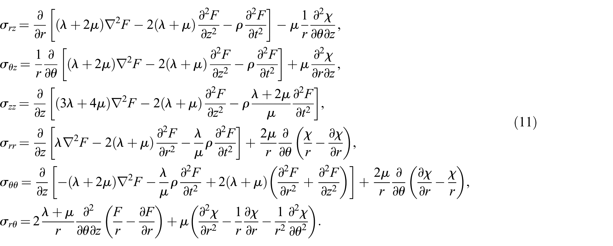
$σ$	Cauchy stress tensor	${\bar{s}}_{R}$	slowness of the Rayleigh surface wave
$x$	position vector	$\bar{s}$	a general slowness constant
$p$	surface traction vector	$a, b$	wave characteristic radicals
$λ, μ$	Lamé elastic constants	$α, β$	scaled wave characteristic radicals
$x_{1}, x_{2}, x_{3}$	Cartesian coordinates	$\tilde{f}$	Laplace transform of $f$
$r, θ, z$	cylindrical coordinates	$\hat{f}$	finite Fourier transform of $f$
$φ_{0}, θ_{0}$	spherical angles of point load application	$f_{H ν}$	Hankel transform of $f$ (of order $v$ )
$R$	spherical radius; $R = \sqrt{r^{2} + z^{2}}$	$s$	Laplace transform parameter
$t, τ$	time and dimensionless time variables	$m$	finite Fourier transform parameter
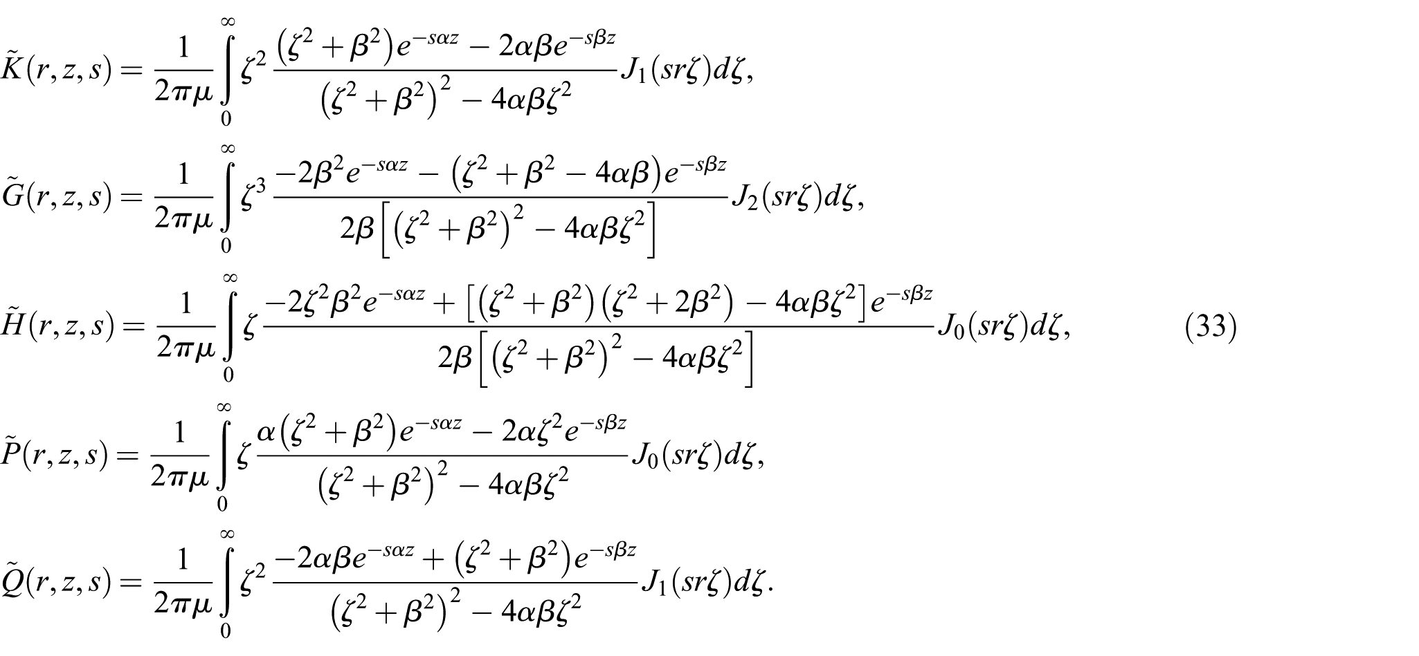
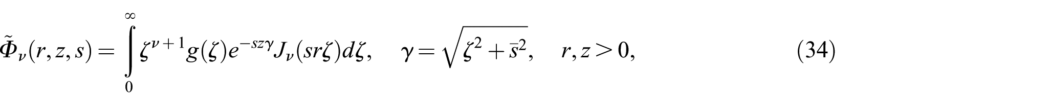
$x$	a dummy integration variable ( $x > 1)$	$ξ$	Hankel transform parameter
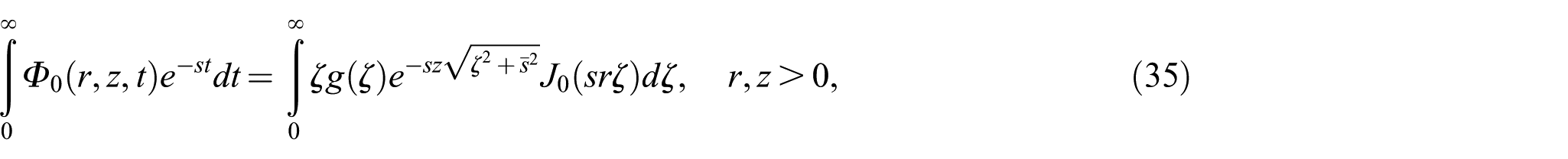
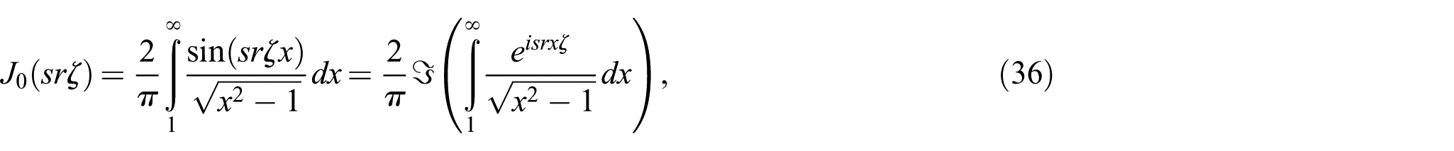
$y$	an auxiliary variable; $y = \sqrt{r^{2} x^{2} + z^{2}}$	$ζ$	scaled Hankel transform parameter
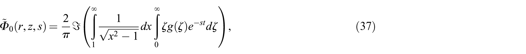
$δ (\cdot)$	Dirac delta function	$u_{r}$	radial component of the displacement vector
$δ_{mn}$	Kronecker’s delta symbol	$u_{θ}$	angular component of the displacement vector
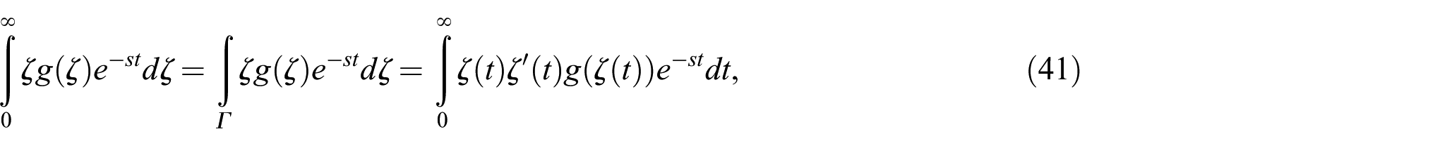
$J_{ν} (\cdot)$	Bessel function of the first kind	$u_{z}$	vertical component of the displacement vector
$ℜ (\cdot)$	real part of a complex quantity	$u_{jk}$	Green’s functions for a Heaviside point source
$ℑ (\cdot)$	imaginary part of a complex quantity	$u_{i (v)}, u_{i (h)}$	displacement due to vertical and horizontal loads

2. Formulation of the initial boundary value problem

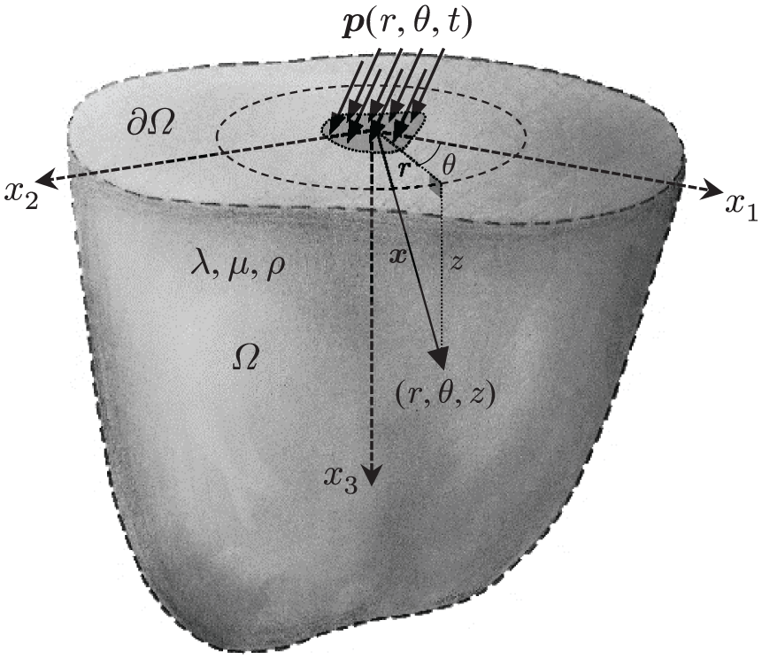
In this section, the initial boundary value problem that is of interest in this paper is precisely described. An isotropic, homogenous, linear elastic solid is considered to occupy a semi-infinite region $Ω$ (a half-space) in the Euclidean space $E^{3}$ . Using a cylindrical coordinate system $(r, θ, z)$ , as shown in Figure 1, the domain of the problem can be represented as $Ω = {x \in E^{3} : z > 0}$ , where x denotes the position vector. In this manner, the plane $z = 0$ defines the boundary $\partial Ω$ of the domain $Ω$ in $E^{3}$ . As depicted in Figure 1, an arbitrary surface traction $p = p (r, θ, t)$ is assumed, for the moment, to be exerted on a finite patch on $\partial Ω$ in the vicinity of the origin. The governing partial differential equations within $Ω$ are the equations of motion for a linear elastic solid [2]; in vector notation, and in the absence of body force fields, they are written as

μ \nabla^{2} u + (λ + μ) \nabla \nabla \cdot u - ρ \frac{\partial^{2} u}{\partial t^{2}} = 0,

(1)

where $λ$ and $μ$ denote Lamé constants [2], $ρ$ represents the mass density of the solid, the vector function $u = u (x, t)$ is the displacement vector field in the medium and t denotes the time variable. As usual, ∇ and $\nabla^{2}$ denote respectively the three-dimensional gradient and Laplacian operators. The medium is assumed to be of quiescent past; accordingly the initial conditions are given by

u (x, 0) = \frac{\partial}{\partial t} u (x, 0) = 0 .

(2)

Figure 1.

A semi-infinite elastic isotropic solid defined by Lamé constants $λ$ and $μ$ disturbed at the boundary by an arbitrary surface traction $p (r, θ, t)$ .

Since the domain is unbounded and the surface traction p is exerted on a finite patch on the boundary, one has to take the regularity conditions into account, which are written as $‖ u (x, t) ‖ \to 0$ as $‖ x ‖ \to \infty$ . Here, as usual, the symbol ‖.‖ stands for the norm of the corresponding vectors. This condition ensures that the mathematical solutions are physically meaningful [25].

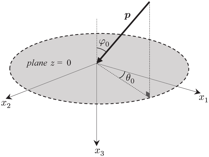
The final step is to delineate the configuration of the excitation source p and the boundary conditions. We are seeking the solutions due to a dynamical point load applied onto $\partial Ω$ with an arbitrary inclination (specified by the angles $φ_{0}$ and $θ_{0}$ ), as illustrated in Figure 2. Without loss of generality, the point load is assumed to be applied at the origin. Hence, the distribution of the surface traction p could be written as

p (r, θ, t) = p (t) \frac{δ (r)}{2 π r} e_{p},

(3)

where $δ (r)$ is the Dirac delta function [26], $e_{p}$ is the unit vector pointing in the direction of vector p and $p (t)$ denotes the time-dependent magnitude of this point load. According to Figure 2, we have

\begin{array}{l} e_{p} = - \cos θ_{0} \sin φ_{0} e_{1} - \sin θ_{0} \sin φ_{0} e_{2} + \cos φ_{0} e_{3} \\ = - \cos (θ - θ_{0}) \sin φ_{0} e_{r} + \sin (θ - θ_{0}) \sin φ_{0} e_{θ} + \cos φ_{0} e_{z}, \end{array}

(4)

in which ${e_{1}, e_{2}, e_{3}}$ and ${e_{r}, e_{θ}, e_{z}}$ stand for, respectively, the unit basis vectors in Cartesian $(x_{1}, x_{2}, x_{3})$ and cylindrical $(r, θ, z)$ coordinates. Hence, the cylindrical components of the point load $p (r, θ, t)$ are

p_{r} = - p (t) \frac{δ (r)}{2 π r} \sin φ_{0} \cos (θ - θ_{0}), p_{θ} = p (t) \frac{δ (r)}{2 π r} \sin φ_{0} \sin (θ - θ_{0}), p_{z} = p (t) \frac{δ (r)}{2 π r} \cos φ_{0} .

(5)

Figure 2.

Configuration of the dynamical surface point load with arbitrary orientation.

With the load configuration assumed as above, the boundary conditions for this problem can be written in terms of three components of the Cauchy stress tensor $σ$ as

σ_{r z} (r, θ, 0^{+}, t) = - p_{r} (r, θ, t), σ_{θ z} (r, θ, 0^{+}, t) = - p_{θ} (r, θ, t), σ_{z z} (r, θ, 0^{+}, t) = - p_{z} (r, θ, t) .

(6)

The symbol $0^{+}$ in the above equations indicates that the corresponding functions are being evaluated at the limit case $z \to 0^{+}$ . Moreover, the stress and displacement components are related via the equation,

σ = λ (\nabla \cdot u) I + μ [\nabla u + {(\nabla u)}^{T}],

(7)

in which I is the second order identity tensor and ${(\cdot)}^{T}$ represents the transpose of a second order tensor. The set of equations (1), (2), and (6), along with the abovementioned regularity conditions, define the desired initial boundary value problem that will be solved analytically in this paper. The final solution consists of the displacement field $u (x, t)$ being given at each $x \in Ω$ and for all $t > 0$ .

3. Potential functions and the method of solution

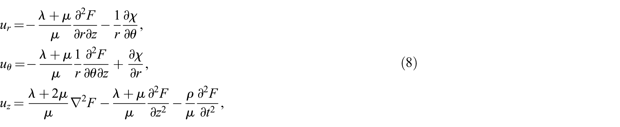
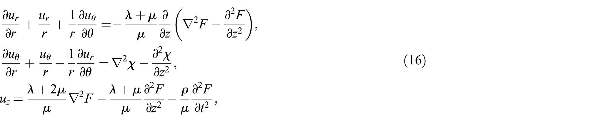
Equation (1) is a system of three coupled partial differential equations, which may be solved with the method of potentials [2, 27]. Here, degenerated versions of the scalar potential functions F and $χ$ , originally developed by Eskandari-Ghadi for transversely isotropic solids [28], are employed. The functions F and $χ$ can be widely applied to various problems ranging from elastostatics to elastodynamics in both isotropic and transversely isotropic media [29]. In a cylindrical coordinate system, the displacements can be represented in terms of the functions F and $χ$ as [28, 29],

\begin{array}{l} u_{r} = - \frac{λ + μ}{μ} \frac{\partial^{2} F}{\partial r \partial z} - \frac{1}{r} \frac{\partial χ}{\partial θ}, \\ u_{θ} = - \frac{λ + μ}{μ} \frac{1}{r} \frac{\partial^{2} F}{\partial θ \partial z} + \frac{\partial χ}{\partial r}, \\ u_{z} = \frac{λ + 2 μ}{μ} \nabla^{2} F - \frac{λ + μ}{μ} \frac{\partial^{2} F}{\partial z^{2}} - \frac{ρ}{μ} \frac{\partial^{2} F}{\partial t^{2}}, \end{array}

(8)

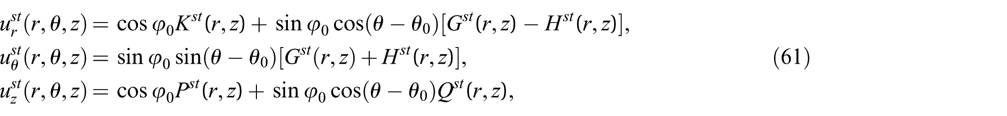
where $F = F (r, θ, z, t)$ and $χ = χ (r, θ, z, t)$ are smooth up to some necessary degree, and satisfy the partial differential equations

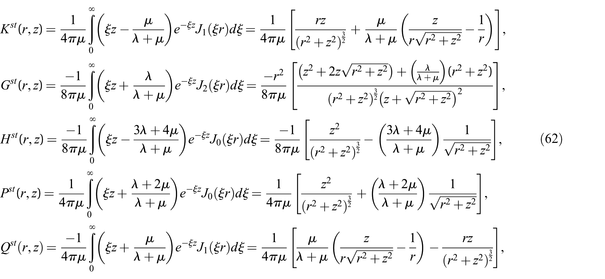
(\nabla^{2} - \frac{1}{c_{L}^{2}} \frac{\partial^{2}}{\partial t^{2}}) (\nabla^{2} - \frac{1}{c_{T}^{2}} \frac{\partial^{2}}{\partial t^{2}}) F (r, θ, z, t) = 0, (\nabla^{2} - \frac{1}{c_{T}^{2}} \frac{\partial^{2}}{\partial t^{2}}) χ (r, θ, z, t) = 0 .

(9)

Here, $c_{L}$ and $c_{T}$ are, respectively, the speeds of propagation for the longitudinal and transverse elastic waves in the medium; see [2] and [25]. These constants are given as

c_{L} = \sqrt{\frac{λ + 2 μ}{ρ}}, c_{T} = \sqrt{\frac{μ}{ρ}} .

(10)

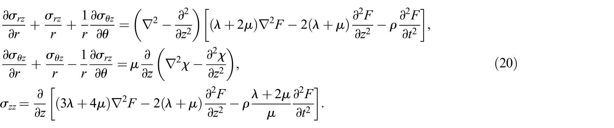
From equation (9), it is evident that the function $χ$ is governed by a three-dimensional wave equation, having the speed of transverse waves, while the function F is governed by a three-dimensional bi-wave equation incorporating both the speeds of longitudinal and transverse waves. Using equations (8) and the stress–displacement relations (equation (7)), one may express the stress components in terms of potential functions as

\begin{matrix} σ_{rz} = \frac{\partial}{\partial r} [(λ + 2 μ) \nabla^{2} F - 2 (λ + μ) \frac{\partial^{2} F}{\partial z^{2}} - ρ \frac{\partial^{2} F}{\partial t^{2}}] - μ \frac{1}{r} \frac{\partial^{2} χ}{\partial θ \partial z}, \\ σ_{θ z} = \frac{1}{r} \frac{\partial}{\partial θ} [(λ + 2 μ) \nabla^{2} F - 2 (λ + μ) \frac{\partial^{2} F}{\partial z^{2}} - ρ \frac{\partial^{2} F}{\partial t^{2}}] + μ \frac{\partial^{2} χ}{\partial r \partial z}, \\ σ_{zz} = \frac{\partial}{\partial z} [(3 λ + 4 μ) \nabla^{2} F - 2 (λ + μ) \frac{\partial^{2} F}{\partial z^{2}} - ρ \frac{λ + 2 μ}{μ} \frac{\partial^{2} F}{\partial t^{2}}], \\ σ_{rr} = \frac{\partial}{\partial z} [λ \nabla^{2} F - 2 (λ + μ) \frac{\partial^{2} F}{\partial r^{2}} - \frac{λ}{μ} ρ \frac{\partial^{2} F}{\partial t^{2}}] + \frac{2 μ}{r} \frac{\partial}{\partial θ} (\frac{χ}{r} - \frac{\partial χ}{\partial r}), \\ σ_{θ θ} = \frac{\partial}{\partial z} [- (λ + 2 μ) \nabla^{2} F - \frac{λ}{μ} ρ \frac{\partial^{2} F}{\partial t^{2}} + 2 (λ + μ) (\frac{\partial^{2} F}{\partial r^{2}} + \frac{\partial^{2} F}{\partial z^{2}})] + \frac{2 μ}{r} \frac{\partial}{\partial θ} (\frac{\partial χ}{\partial r} - \frac{χ}{r}), \\ σ_{r θ} = 2 \frac{λ + μ}{r} \frac{\partial^{2}}{\partial θ \partial z} (\frac{F}{r} - \frac{\partial F}{\partial r}) + μ (\frac{\partial^{2} χ}{\partial r^{2}} - \frac{1}{r} \frac{\partial χ}{\partial r} - \frac{1}{r^{2}} \frac{\partial^{2} χ}{\partial θ^{2}}) . \end{matrix}

(11)

In axisymmetric problems, the function $χ$ can be eliminated and thus all the displacements and stresses will be expressible in terms of the function F, solely [28]. The solution method followed in the ensuing is the application of Laplace, finite exponential Fourier and Hankel integral transforms with respect to the temporal, angular, and radial variables (t, $θ$ and r), respectively. Accordingly, the partial differential equations (9) can be reduced to ordinary differential equations (in terms of z) for which the general solutions can be found. Subsequently, upon expressing the boundary conditions of equation (6) in the triply-transformed domain, the unknown constants in these general solutions can be fully determined. Lastly, the inversion of the solutions from the triply-transformed domain to the physical domain is ought to be carried out. This has proven to be an arduous task in previous studies; hence, it will be meticulously studied in our discussions.

4. Analytical solution of the problem

The analytical solution of the initial boundary value problem is thoroughly examined in this section. For a more organised discussion, this section is divided into several subsections as follows.

4.1. General solution for the potential functions F and $χ$

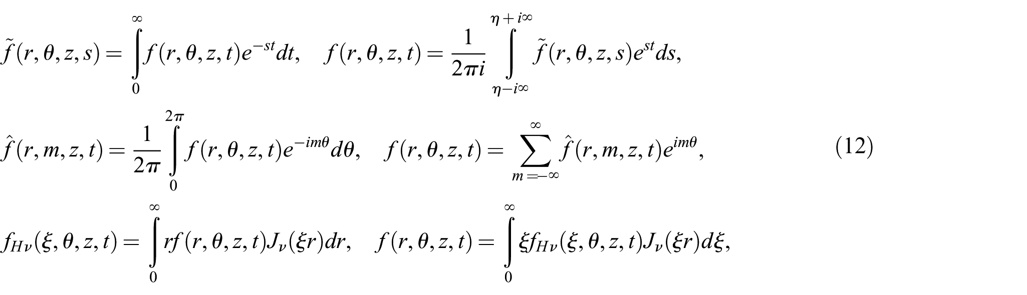
In this research, we are concerned with real-valued functions of four variables (three spatial and one temporal). Let us represent a generic function of this form by $f (r, θ, z, t)$ where $r, z, t \geq 0$ , $- \infty < θ < \infty$ , and further assume that $f (r, θ, z, t)$ is continuous and periodic with respect to $θ$ with the period of $2 π$ and of exponential order with respect to t as $t \to \infty$ . The Laplace, finite exponential Fourier and Hankel transforms of $f (r, θ, z, t)$ with respect to t, $θ$ and r, along with their inversion formulae are represented by (see [13, 26, 30] for details)

\begin{matrix} \tilde{f} (r, θ, z, s) = \int_{0}^{\infty} f (r, θ, z, t) e^{- st} dt, f (r, θ, z, t) = \frac{1}{2 π i} \int_{η - i \infty}^{η + i \infty} \tilde{f} (r, θ, z, s) e^{st} ds, \\ \hat{f} (r, m, z, t) = \frac{1}{2 π} \int_{0}^{2 π} f (r, θ, z, t) e^{- im θ} d θ, f (r, θ, z, t) = \sum_{m = - \infty}^{\infty} \hat{f} (r, m, z, t) e^{im θ}, \\ f_{H ν} (ξ, θ, z, t) = \int_{0}^{\infty} rf (r, θ, z, t) J_{ν} (ξ r) dr, f (r, θ, z, t) = \int_{0}^{\infty} ξ f_{H ν} (ξ, θ, z, t) J_{ν} (ξ r) d ξ, \end{matrix}

(12)

respectively. Here s, a real or complex number, is the Laplace transform parameter, and $η$ is an arbitrary real number for which $\tilde{f} (r, θ, z, s)$ is an analytic complex-valued function of s throughout the half-plane $ℜ (s) > η$ in the complex s-plane. Similarly, $m \in Z$ and $ξ > 0$ are respectively the Fourier and Hankel transform parameters. Finally, $J_{ν} (\cdot)$ denotes the Bessel function of the first kind and of order $ν$ [31], and the symbols $ℜ (\cdot)$ and $ℑ (\cdot)$ shall stand for the real and imaginary parts of a complex number, respectively. By using the integrals transforms (12) in succession, one obtains the function ${\hat{\tilde{f}}}_{H ν} (ξ, m, z, s)$ that represents $f (r, θ, z, t)$ in the triply-transformed domain.

We can now proceed to the solution of equations given in equation (9). Taking the Laplace, Fourier and mth order Hankel integral transforms from both sides of equation (9), and using zero initial conditions for functions F and $χ$ , which is in conformity with the original initial conditions as given in equation (2) for the problem, the ordinary differential equations

(\frac{\partial^{2}}{\partial z^{2}} - a^{2}) (\frac{\partial^{2}}{\partial z^{2}} - b^{2}) {\hat{\tilde{F}}}_{Hm} (ξ, m, z, s) = 0, (\frac{\partial^{2}}{\partial z^{2}} - b^{2}) {\hat{\tilde{χ}}}_{Hm} (ξ, m, z, s) = 0,

(13)

are found, in which the functions a and b, defined by

a = a (ξ, s) = \sqrt{ξ^{2} + {\bar{s}}_{L}^{2} s^{2}}, b = b (ξ, s) = \sqrt{ξ^{2} + {\bar{s}}_{T}^{2} s^{2}},

(14)

denote the characteristic radicals of longitudinal and transverse waves. In the above equation, ${\bar{s}}_{L} = 1 / c_{L}$ and ${\bar{s}}_{T} = 1 / c_{T}$ are the wave slowness constants for longitudinal and transverse elastic waves, respectively [2]. The general solutions for the equations (13), which are compatible with the regularity conditions, are

{\hat{\tilde{F}}}_{Hm} (ξ, m, z, s) = A (ξ, m, s) e^{- az} + B (ξ, m, s) e^{- bz}, {\hat{\tilde{χ}}}_{Hm} (ξ, m, z, s) = C (ξ, m, s) e^{- bz} .

(15)

In the above equations, the functions A, B and C will be determined by satisfying the boundary conditions.

4.2. Boundary conditions in the triply-transformed domain

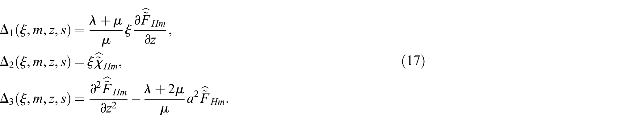
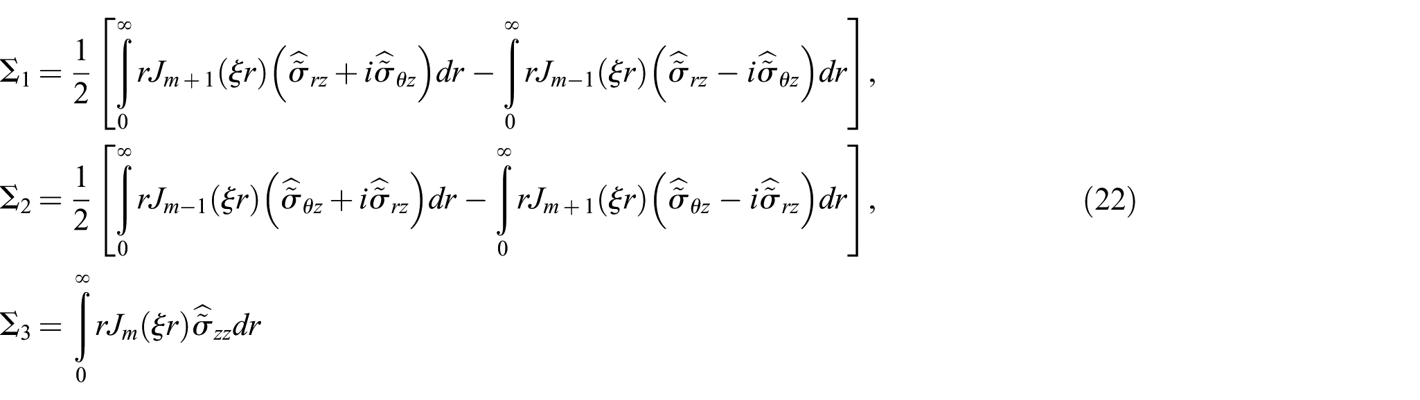
A number of auxiliary functions are defined in this section in such a way that they indirectly represent the displacements, stresses and excitations in the triply-transformed domain. These functions enable us to express the boundary conditions directly in terms of the potential functions in the triply-transformed domain. Upon differentiation and linear combination of equations (8), it can be inferred that

\begin{matrix} \frac{\partial u_{r}}{\partial r} + \frac{u_{r}}{r} + \frac{1}{r} \frac{\partial u_{θ}}{\partial θ} = - \frac{λ + μ}{μ} \frac{\partial}{\partial z} (\nabla^{2} F - \frac{\partial^{2} F}{\partial z^{2}}), \\ \frac{\partial u_{θ}}{\partial r} + \frac{u_{θ}}{r} - \frac{1}{r} \frac{\partial u_{r}}{\partial θ} = \nabla^{2} χ - \frac{\partial^{2} χ}{\partial z^{2}}, \\ u_{z} = \frac{λ + 2 μ}{μ} \nabla^{2} F - \frac{λ + μ}{μ} \frac{\partial^{2} F}{\partial z^{2}} - \frac{ρ}{μ} \frac{\partial^{2} F}{\partial t^{2}}, \end{matrix}

(16)

based on which one finds by applying successively the Laplace, Fourier and mth order Hankel transforms

\begin{matrix} Δ_{1} (ξ, m, z, s) = \frac{λ + μ}{μ} ξ \frac{\partial {\hat{\tilde{F}}}_{Hm}}{\partial z}, \\ Δ_{2} (ξ, m, z, s) = ξ {\hat{\tilde{χ}}}_{Hm}, \\ Δ_{3} (ξ, m, z, s) = \frac{\partial^{2} {\hat{\tilde{F}}}_{Hm}}{\partial z^{2}} - \frac{λ + 2 μ}{μ} a^{2} {\hat{\tilde{F}}}_{Hm} . \end{matrix}

(17)

where we define

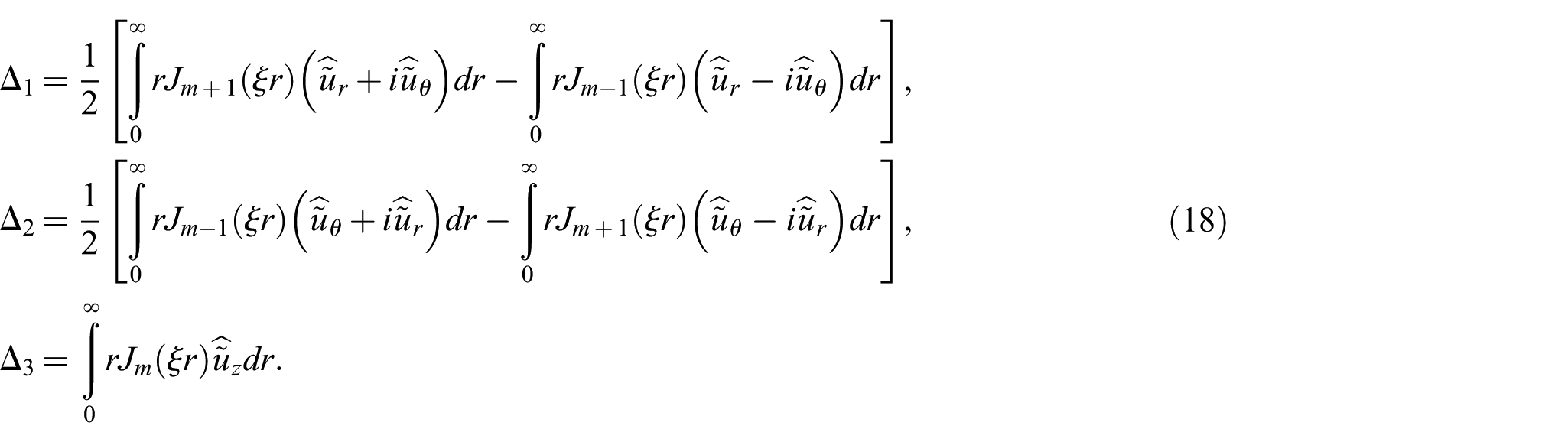
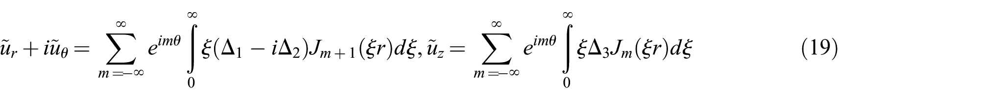
\begin{matrix} Δ_{1} = \frac{1}{2} [\int_{0}^{\infty} r J_{m + 1} (ξ r) ({\hat{\tilde{u}}}_{r} + i {\hat{\tilde{u}}}_{θ}) dr - \int_{0}^{\infty} r J_{m - 1} (ξ r) ({\hat{\tilde{u}}}_{r} - i {\hat{\tilde{u}}}_{θ}) dr], \\ Δ_{2} = \frac{1}{2} [\int_{0}^{\infty} r J_{m - 1} (ξ r) ({\hat{\tilde{u}}}_{θ} + i {\hat{\tilde{u}}}_{r}) dr - \int_{0}^{\infty} r J_{m + 1} (ξ r) ({\hat{\tilde{u}}}_{θ} - i {\hat{\tilde{u}}}_{r}) dr], \\ Δ_{3} = \int_{0}^{\infty} r J_{m} (ξ r) {\hat{\tilde{u}}}_{z} dr . \end{matrix}

(18)

$Δ_{j}$ ( $j = 1, 2, 3$ ) are three auxiliary functions for displacements. From the above equations and by applying the inversion formulae of finite Fourier and Hankel transforms given by equation (12), it can be deduced that

{\tilde{u}}_{r} + i {\tilde{u}}_{θ} = \sum_{m = - \infty}^{\infty} e^{im θ} \int_{0}^{\infty} ξ (Δ_{1} - i Δ_{2}) J_{m + 1} (ξ r) d ξ, {\tilde{u}}_{z} = \sum_{m = - \infty}^{\infty} e^{im θ} \int_{0}^{\infty} ξ Δ_{3} J_{m} (ξ r) d ξ

(19)

In a similar manner from the first three relations given in equation (11), it is easy to deduce that

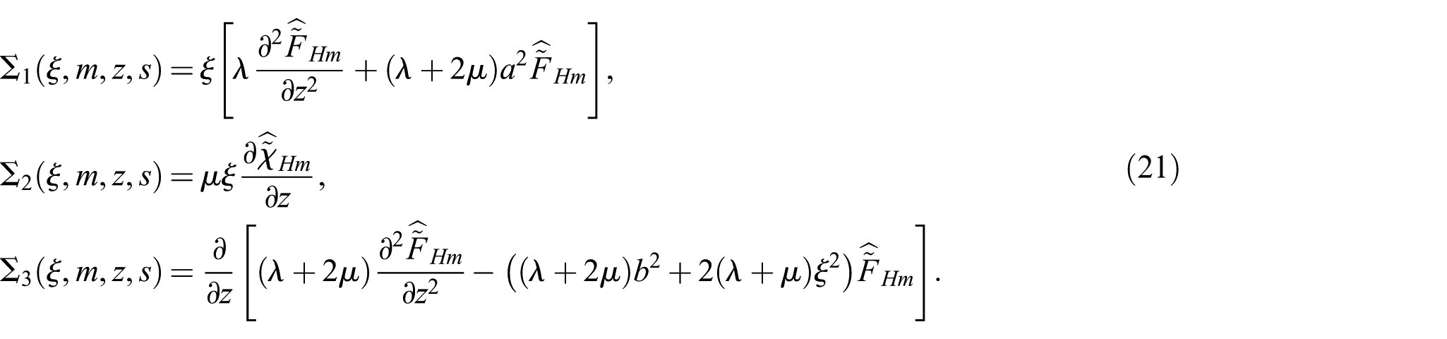
\begin{matrix} \frac{\partial σ_{rz}}{\partial r} + \frac{σ_{rz}}{r} + \frac{1}{r} \frac{\partial σ_{θ z}}{\partial θ} = (\nabla^{2} - \frac{\partial^{2}}{\partial z^{2}}) [(λ + 2 μ) \nabla^{2} F - 2 (λ + μ) \frac{\partial^{2} F}{\partial z^{2}} - ρ \frac{\partial^{2} F}{\partial t^{2}}], \\ \frac{\partial σ_{θ z}}{\partial r} + \frac{σ_{θ z}}{r} - \frac{1}{r} \frac{\partial σ_{rz}}{\partial θ} = μ \frac{\partial}{\partial z} (\nabla^{2} χ - \frac{\partial^{2} χ}{\partial z^{2}}), \\ σ_{zz} = \frac{\partial}{\partial z} [(3 λ + 4 μ) \nabla^{2} F - 2 (λ + μ) \frac{\partial^{2} F}{\partial z^{2}} - ρ \frac{λ + 2 μ}{μ} \frac{\partial^{2} F}{\partial t^{2}}] . \end{matrix}

(20)

By implementing the Laplace, Fourier and mth order Hankel integral transforms successively, one finds

\begin{matrix} Σ_{1} (ξ, m, z, s) = ξ [λ \frac{\partial^{2} {\hat{\tilde{F}}}_{Hm}}{\partial z^{2}} + (λ + 2 μ) a^{2} {\hat{\tilde{F}}}_{Hm}], \\ Σ_{2} (ξ, m, z, s) = μ ξ \frac{\partial {\hat{\tilde{χ}}}_{Hm}}{\partial z}, \\ Σ_{3} (ξ, m, z, s) = \frac{\partial}{\partial z} [(λ + 2 μ) \frac{\partial^{2} {\hat{\tilde{F}}}_{Hm}}{\partial z^{2}} - ((λ + 2 μ) b^{2} + 2 (λ + μ) ξ^{2}) {\hat{\tilde{F}}}_{Hm}] . \end{matrix}

(21)

in which

\begin{matrix} Σ_{1} = \frac{1}{2} [\int_{0}^{\infty} r J_{m + 1} (ξ r) ({\hat{\tilde{σ}}}_{rz} + i {\hat{\tilde{σ}}}_{θ z}) dr - \int_{0}^{\infty} r J_{m - 1} (ξ r) ({\hat{\tilde{σ}}}_{rz} - i {\hat{\tilde{σ}}}_{θ z}) dr], \\ Σ_{2} = \frac{1}{2} [\int_{0}^{\infty} r J_{m - 1} (ξ r) ({\hat{\tilde{σ}}}_{θ z} + i {\hat{\tilde{σ}}}_{rz}) dr - \int_{0}^{\infty} r J_{m + 1} (ξ r) ({\hat{\tilde{σ}}}_{θ z} - i {\hat{\tilde{σ}}}_{rz}) dr], \\ Σ_{3} = \int_{0}^{\infty} r J_{m} (ξ r) {\hat{\tilde{σ}}}_{zz} dr \end{matrix}

(22)

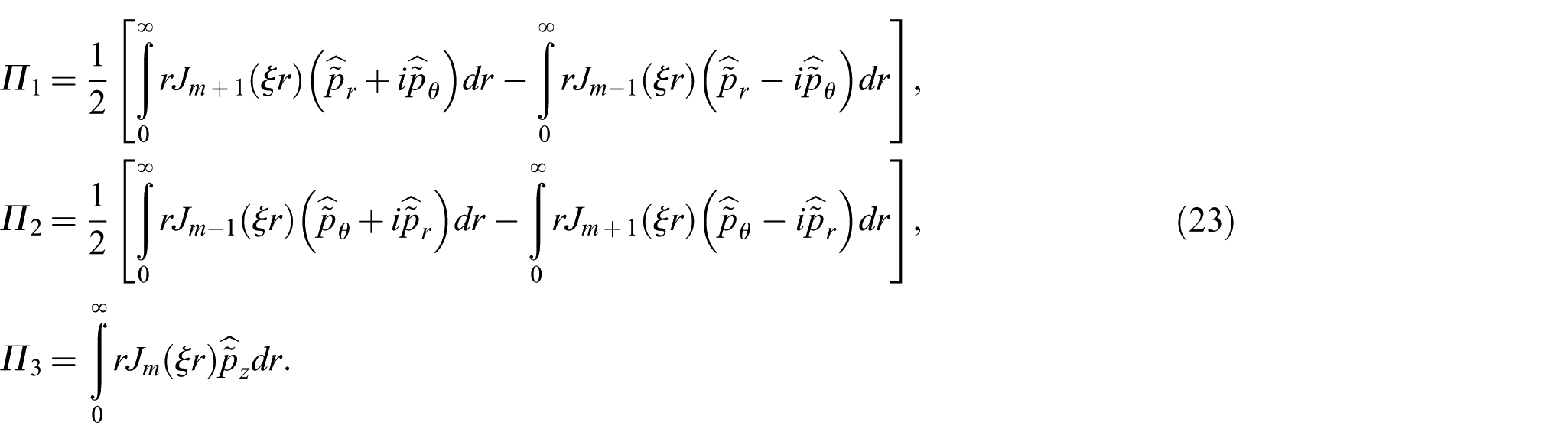
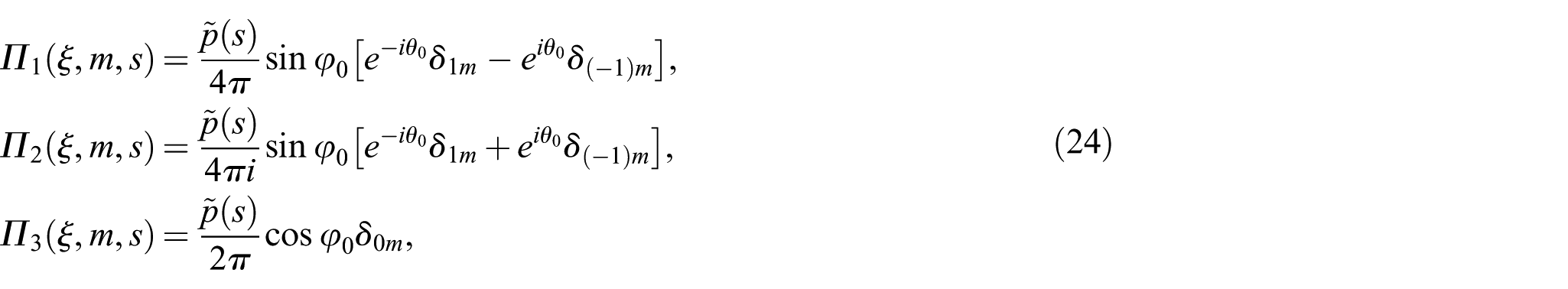
The auxiliary functions $Σ_{j}$ ( $j = 1, 2, 3$ ) are defined in connection with the stress components $σ_{rz}$ , $σ_{θ z}$ and $σ_{zz}$ that appear in the boundary conditions of equation (6). Analogously, the auxiliary functions $Π_{j}$ ( $j = 1, 2, 3$ ) can be defined in connection with the components of the vector p as

\begin{matrix} Π_{1} = \frac{1}{2} [\int_{0}^{\infty} r J_{m + 1} (ξ r) ({\hat{\tilde{p}}}_{r} + i {\hat{\tilde{p}}}_{θ}) dr - \int_{0}^{\infty} r J_{m - 1} (ξ r) ({\hat{\tilde{p}}}_{r} - i {\hat{\tilde{p}}}_{θ}) dr], \\ Π_{2} = \frac{1}{2} [\int_{0}^{\infty} r J_{m - 1} (ξ r) ({\hat{\tilde{p}}}_{θ} + i {\hat{\tilde{p}}}_{r}) dr - \int_{0}^{\infty} r J_{m + 1} (ξ r) ({\hat{\tilde{p}}}_{θ} - i {\hat{\tilde{p}}}_{r}) dr], \\ Π_{3} = \int_{0}^{\infty} r J_{m} (ξ r) {\hat{\tilde{p}}}_{z} dr . \end{matrix}

(23)

By substitution of $p_{r}$ , $p_{θ}$ and $p_{z}$ from equation (5) into the above definitions, the formulae

\begin{matrix} Π_{1} (ξ, m, s) = \frac{\tilde{p} (s)}{4 π} \sin φ_{0} [e^{- i θ_{0}} δ_{1 m} - e^{i θ_{0}} δ_{(- 1) m}], \\ Π_{2} (ξ, m, s) = \frac{\tilde{p} (s)}{4 π i} \sin φ_{0} [e^{- i θ_{0}} δ_{1 m} + e^{i θ_{0}} δ_{(- 1) m}], \\ Π_{3} (ξ, m, s) = \frac{\tilde{p} (s)}{2 π} \cos φ_{0} δ_{0 m}, \end{matrix}

(24)

are found where $\tilde{p} (s)$ stands for the Laplace transform of $p (t)$ and $δ_{nm}$ represents a generalised version of Kronecker’s delta for which $m, n \in Z$ . Having defined the auxiliary functions, the boundary conditions for the functions ${\hat{\tilde{F}}}_{Hm}$ and ${\hat{\tilde{χ}}}_{Hm}$ shall be conveniently found in the triply-transformed domain. To this end, the boundary equations (6) can be transformed and manipulated in accordance with equations (22) and (23) to acquire

Σ_{1} (ξ, m, 0^{+}, s) = - Π_{1} (ξ, m, s), Σ_{2} (ξ, m, 0^{+}, s) = - Π_{2} (ξ, m, s), Σ_{3} (ξ, m, 0^{+}, s) = - Π_{3} (ξ, m, s) .

(25)

Lastly indeed, from equations (15), (17) and (21), one infers after some manipulations that

\begin{matrix} Δ_{1} = - \frac{λ + μ}{μ} ξ (aA e^{- az} + bB e^{- bz}), Σ_{1} = ξ (λ + μ) [2 a^{2} A e^{- az} + B e^{- bz} (ξ^{2} + b^{2})], \\ Δ_{2} = ξ C e^{- bz}, Σ_{2} = - ξ μ bC e^{- bz}, \\ Δ_{3} = - \frac{λ + μ}{μ} (a^{2} A e^{- az} + ξ^{2} B e^{- bz}), Σ_{3} = (λ + μ) [(ξ^{2} + b^{2}) aA e^{- az} + 2 ξ^{2} bB e^{- bz}] . \end{matrix}

(26)

4.3. Laplace-domain displacement components

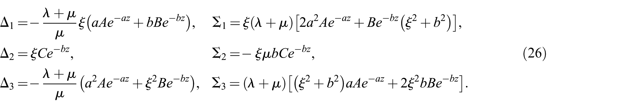
By substituting $Σ_{j}$ from equations (26) into the transformed boundary conditions of equation (25), a system of linear algebraic equations is deduced in the form of

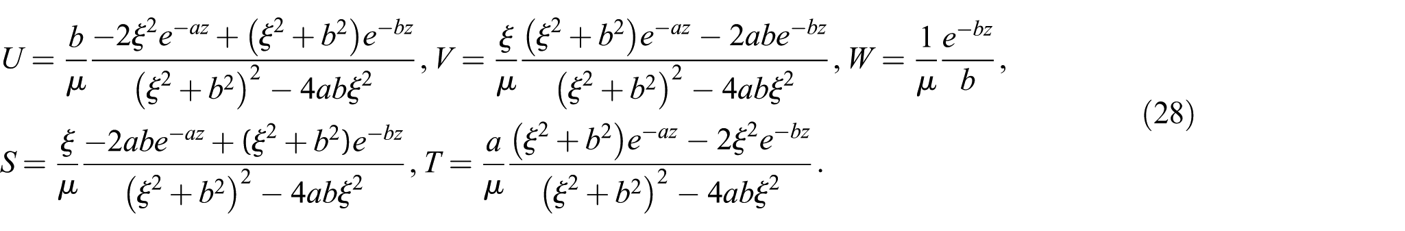
2 a^{2} A + B (ξ^{2} + b^{2}) = - \frac{Π_{1}}{ξ (λ + μ)}, ξ μ bC = Π_{2}, (ξ^{2} + b^{2}) aA + 2 ξ^{2} bB = - \frac{Π_{3}}{λ + μ} .

(27)

These equations can be readily solved for A, B and C. Substituting the results into equations (26), one may find the auxiliary displacements $Δ_{j}$ as $Δ_{1} = U Π_{1} + V Π_{3}$ , $Δ_{2} = W Π_{2}$ , and $Δ_{3} = S Π_{1} + T Π_{3}$ , where

\begin{matrix} U = \frac{b}{μ} \frac{- 2 ξ^{2} e^{- az} + (ξ^{2} + b^{2}) e^{- bz}}{{(ξ^{2} + b^{2})}^{2} - 4 ab ξ^{2}}, V = \frac{ξ}{μ} \frac{(ξ^{2} + b^{2}) e^{- az} - 2 ab e^{- bz}}{{(ξ^{2} + b^{2})}^{2} - 4 ab ξ^{2}}, W = \frac{1}{μ} \frac{e^{- bz}}{b}, \\ S = \frac{ξ}{μ} \frac{- 2 ab e^{- az} + (ξ^{2} + b^{2}) e^{- bz}}{{(ξ^{2} + b^{2})}^{2} - 4 ab ξ^{2}}, T = \frac{a}{μ} \frac{(ξ^{2} + b^{2}) e^{- az} - 2 ξ^{2} e^{- bz}}{{(ξ^{2} + b^{2})}^{2} - 4 ab ξ^{2}} . \end{matrix}

(28)

On the other hand, by substituting $Δ_{j}$ in these forms in the equations (19) while using equation (24), one finds after some tedious manipulations the formulae

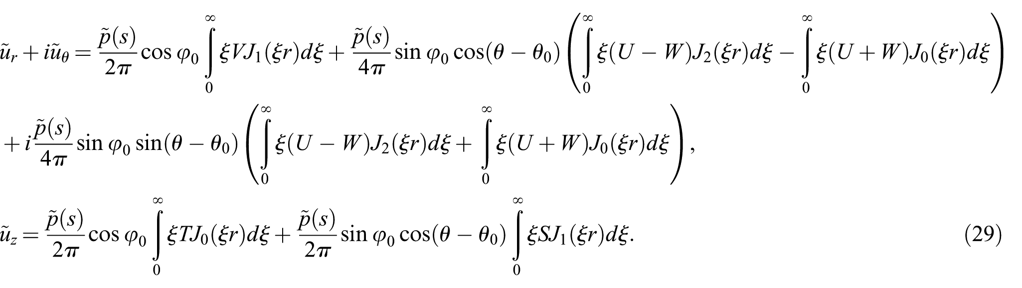
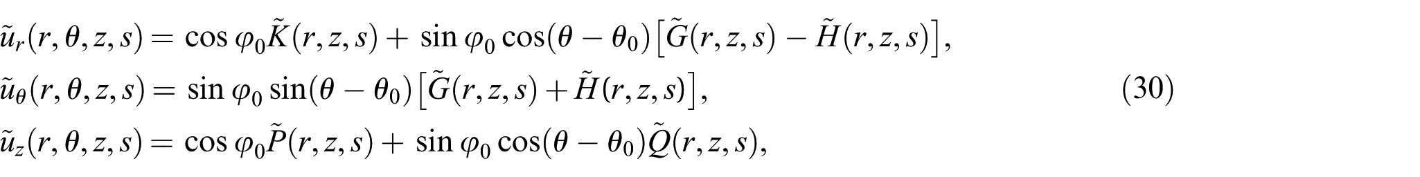
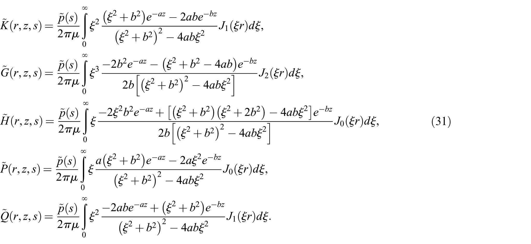
\begin{matrix} {\tilde{u}}_{r} + i {\tilde{u}}_{θ} = \frac{\tilde{p} (s)}{2 π} \cos φ_{0} \int_{0}^{\infty} ξ V J_{1} (ξ r) d ξ + \frac{\tilde{p} (s)}{4 π} \sin φ_{0} \cos (θ - θ_{0}) (\int_{0}^{\infty} ξ (U - W) J_{2} (ξ r) d ξ - \int_{0}^{\infty} ξ (U + W) J_{0} (ξ r) d ξ) \\ + i \frac{\tilde{p} (s)}{4 π} \sin φ_{0} \sin (θ - θ_{0}) (\int_{0}^{\infty} ξ (U - W) J_{2} (ξ r) d ξ + \int_{0}^{\infty} ξ (U + W) J_{0} (ξ r) d ξ), \\ {\tilde{u}}_{z} = \frac{\tilde{p} (s)}{2 π} \cos φ_{0} \int_{0}^{\infty} ξ T J_{0} (ξ r) d ξ + \frac{\tilde{p} (s)}{2 π} \sin φ_{0} \cos (θ - θ_{0}) \int_{0}^{\infty} ξ S J_{1} (ξ r) d ξ . \end{matrix}

(29)

Finally, from the equations (28) and (29), and noticing that all the occurring integrals are real-valued, it is straightforward to find the Laplace-domain displacement components as

\begin{matrix} {\tilde{u}}_{r} (r, θ, z, s) = \cos φ_{0} \tilde{K} (r, z, s) + \sin φ_{0} \cos (θ - θ_{0}) [\tilde{G} (r, z, s) - \tilde{H} (r, z, s)], \\ {\tilde{u}}_{θ} (r, θ, z, s) = \sin φ_{0} \sin (θ - θ_{0}) [\tilde{G} (r, z, s) + \tilde{H} (r, z, s)], \\ {\tilde{u}}_{z} (r, θ, z, s) = \cos φ_{0} \tilde{P} (r, z, s) + \sin φ_{0} \cos (θ - θ_{0}) \tilde{Q} (r, z, s), \end{matrix}

(30)

in which

\begin{matrix} \tilde{K} (r, z, s) = \frac{\tilde{p} (s)}{2 π μ} \int_{0}^{\infty} ξ^{2} \frac{(ξ^{2} + b^{2}) e^{- az} - 2 ab e^{- bz}}{{(ξ^{2} + b^{2})}^{2} - 4 ab ξ^{2}} J_{1} (ξ r) d ξ, \\ \tilde{G} (r, z, s) = \frac{\tilde{p} (s)}{2 π μ} \int_{0}^{\infty} ξ^{3} \frac{- 2 b^{2} e^{- az} - (ξ^{2} + b^{2} - 4 ab) e^{- bz}}{2 b [{(ξ^{2} + b^{2})}^{2} - 4 ab ξ^{2}]} J_{2} (ξ r) d ξ, \\ \tilde{H} (r, z, s) = \frac{\tilde{p} (s)}{2 π μ} \int_{0}^{\infty} ξ \frac{- 2 ξ^{2} b^{2} e^{- az} + [(ξ^{2} + b^{2}) (ξ^{2} + 2 b^{2}) - 4 ab ξ^{2}] e^{- bz}}{2 b [{(ξ^{2} + b^{2})}^{2} - 4 ab ξ^{2}]} J_{0} (ξ r) d ξ, \\ \tilde{P} (r, z, s) = \frac{\tilde{p} (s)}{2 π μ} \int_{0}^{\infty} ξ \frac{a (ξ^{2} + b^{2}) e^{- az} - 2 a ξ^{2} e^{- bz}}{{(ξ^{2} + b^{2})}^{2} - 4 ab ξ^{2}} J_{0} (ξ r) d ξ, \\ \tilde{Q} (r, z, s) = \frac{\tilde{p} (s)}{2 π μ} \int_{0}^{\infty} ξ^{2} \frac{- 2 ab e^{- az} + (ξ^{2} + b^{2}) e^{- bz}}{{(ξ^{2} + b^{2})}^{2} - 4 ab ξ^{2}} J_{1} (ξ r) d ξ . \end{matrix}

(31)

The time dependence $p (t)$ of the point load is here chosen to be the unit step function of Heaviside (as in [7], [12], and later researches). Doing so results in $\tilde{p} (s) = s^{- 1}$ in all of the equations (31), and this leads to certain simplifications in the analysis, as will be seen shortly. It should be observed that apart from the factor $\tilde{p} (s)$ , the Laplace transform parameter s occurs elsewhere in these integrals only within the radicals a and b (refer to equations (14)).

By fixing $φ_{0} = 0$ in equation (30), which according to Figure 2 corresponds to a vertical point load in the positive direction of the $x_{3}$ -axis, one may readily verify that the Laplace-domain solutions presented here become equal to the axisymmetric operational solutions of Pekeris [7] in their more complete form given in Achenbach’s treatise [2]. On the other hand, by fixing $φ_{0} = π / 2$ and $θ_{0} = π$ in (30), which corresponds to a horizontal point load in the positive direction of $x_{1}$ -axis, it can be shown that the relations given here are equivalent to those given by Chao [12]. It is emphasised that Lamb, Pekeris, Chao, and many other contributors (see for example [14, 24] ) were essentially interested in the solutions on the boundary of the medium and thus fixed $z = 0$ in their analyses. Among the authors who treated Lamb’s problem for a vertical point load in the case $z > 0$ (inside the half-space), Eason [16], Gakenheimer and Miklowitz (see [17] and [19] ) and Johnson [21] should be mentioned.

4.4. General discussion on the Laplace transform inversion method

In principle, it is possible to directly use the second formula in equation (12) for inversion of the Laplace transform in order to find time-domain representations of the integrals of equations (31). From a computational standpoint, yet, this method, as used by Eason [16], is very laborious since it involves double integration (one of which is an integration in the complex s-plane) and also because of the problematic nature of the wave characteristic radicals a and b. These radicals contain both $ξ$ and s, and they become multivalued relations when s is assumed to be a complex variable. A more sophisticated approach is the technique generally referred to as Cagniard’s method. This involves the substitution $ξ = s ζ$ , that is scaling the Hankel transform parameter $ξ$ with the Laplace transform parameter s, and alterations of integration path in the complex $ζ$ -plane in such a way that the Laplace transform inversion is made possible by mere inspection, without ever involving the Laplace inversion formula in equation (12). Since in this method, the Laplace transform inversion formula is never employed, the parameter s is strictly assumed to be real and positive. By implementing $ξ = s ζ$ , it is readily seen that the characteristic radicals a and b, as given in equation (14), transform into $s α$ and $s β$ , respectively, where we define

α = α (ζ) = \sqrt{ζ^{2} + {\bar{s}}_{L}^{2}}, β = β (ζ) = \sqrt{ζ^{2} + {\bar{s}}_{T}^{2}},

(32)

as scaled characteristic radicals for longitudinal and transverse waves, respectively. Hence, for a point load of Heaviside time dependence, the integrals in (31) are converted into

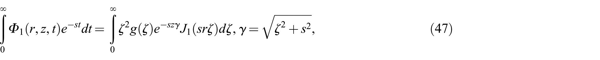
\begin{matrix} \tilde{K} (r, z, s) = \frac{1}{2 π μ} \int_{0}^{\infty} ζ^{2} \frac{(ζ^{2} + β^{2}) e^{- s α z} - 2 α β e^{- s β z}}{{(ζ^{2} + β^{2})}^{2} - 4 α β ζ^{2}} J_{1} (sr ζ) d ζ, \\ \tilde{G} (r, z, s) = \frac{1}{2 π μ} \int_{0}^{\infty} ζ^{3} \frac{- 2 β^{2} e^{- s α z} - (ζ^{2} + β^{2} - 4 α β) e^{- s β z}}{2 β [{(ζ^{2} + β^{2})}^{2} - 4 α β ζ^{2}]} J_{2} (sr ζ) d ζ, \\ \tilde{H} (r, z, s) = \frac{1}{2 π μ} \int_{0}^{\infty} ζ \frac{- 2 ζ^{2} β^{2} e^{- s α z} + [(ζ^{2} + β^{2}) (ζ^{2} + 2 β^{2}) - 4 α β ζ^{2}] e^{- s β z}}{2 β [{(ζ^{2} + β^{2})}^{2} - 4 α β ζ^{2}]} J_{0} (sr ζ) d ζ, \\ \tilde{P} (r, z, s) = \frac{1}{2 π μ} \int_{0}^{\infty} ζ \frac{α (ζ^{2} + β^{2}) e^{- s α z} - 2 α ζ^{2} e^{- s β z}}{{(ζ^{2} + β^{2})}^{2} - 4 α β ζ^{2}} J_{0} (sr ζ) d ζ, \\ \tilde{Q} (r, z, s) = \frac{1}{2 π μ} \int_{0}^{\infty} ζ^{2} \frac{- 2 α β e^{- s α z} + (ζ^{2} + β^{2}) e^{- s β z}}{{(ζ^{2} + β^{2})}^{2} - 4 α β ζ^{2}} J_{1} (sr ζ) d ζ . \end{matrix}

(33)

It is clear that with this change of variable, s appears only in the argument of exponential and Bessel functions as parts of integrands. It is also noticed that each of the integrals involved in equations (33) can be expressed as the sum of two integrals of the following general form

{\tilde{Φ}}_{ν} (r, z, s) = \int_{0}^{\infty} ζ^{ν + 1} g (ζ) e^{- sz γ} J_{ν} (sr ζ) d ζ, γ = \sqrt{ζ^{2} + {\bar{s}}^{2}}, r, z > 0,

(34)

where $γ$ symbolises the scaled characteristic radical of the corresponding wave (being either $α$ or $β$ here), $\bar{s}$ denotes a wave slowness constant ( ${\bar{s}}_{L}$ for $γ = α$ and ${\bar{s}}_{T}$ for $γ = β$ ), and $ν$ is a non-negative integer that occurs only in the cases $ν = 0, 1, 2$ in our study. Moreover, $g (ζ)$ represents a function of $ζ$ , which varies rationally in terms of $ζ^{2}$ , $α (ζ)$ and $β (ζ)$ . The integral given in equation (34) will be referred to as an emission integral (EI) of order $ν$ , hereafter. Physically, ${\tilde{Φ}}_{ν} (r, z, s)$ represents the Laplace transform of a transient wavefront $Φ_{ν} (r, z, t)$ that is being emitted with the slowness $\bar{s}$ in the positive direction of r and z. With this notion, each integral in equations (33) is simply the sum of a longitudinal and a transverse EI. It will be shown that finding the inverse Laplace transform of an EI results in another integral that forms a part of the physical solution of the problem. In the ensuing we study the Laplace transform inversion of EIs of order $ν = 0$ . Treatment of the cases $ν = 1$ and 2 can be easily based on the case $ν = 0$ , afterwards.

4.5. Inverse Laplace transforms of EIs of order $ν = 0$

Seeking the inverse Laplace transform of the function ${\tilde{Φ}}_{0} (r, z, s)$ , as given in (34), is equivalent to solving the integral equation

\int_{0}^{\infty} Φ_{0} (r, z, t) e^{- st} dt = \int_{0}^{\infty} ζ g (ζ) e^{- sz \sqrt{ζ^{2} + {\bar{s}}^{2}}} J_{0} (sr ζ) d ζ, r, z > 0,

(35)

for $Φ_{0} (r, z, t)$ . This integral equation can be solved by the ingenious idea behind the method of Cagniard. Pekeris encountered this integral equation for $ν = 0$ and 1 in many of his investigations in the field of electromagnetic, acoustic and elastic wave propagation (see, e.g. [9]), and he found solutions, which were later summarised in a separate paper [22]. Longman generalised Pekeris’ work for a similar integral equation containing two radicals in the exponent rather than one [23], as occurs in problems involving the reflexion or refraction of waves. The solutions of Pekeris and Longman does not contain the case $ν = 2$ , though. Our method is essentially based on Pekeris’ version of Cagniard’s method with some new modifications in order to derive and represent the solutions in simpler and clearer forms. The essence of Cagniard’s idea is converting the EI into the form of a Laplace transform. Then, the integrands of the Laplace transform integrals on the left- and right-hand sides of equation (35) can be considered equal, essentially, owing to the uniqueness of the Laplace transforms, and consequently $Φ_{0} (r, z, t)$ will be at hand. Having this goal in mind, we use the Mehler–Sonine representation of the zero-order Bessel function of the first kind [31]

J_{0} (sr ζ) = \frac{2}{π} \int_{1}^{\infty} \frac{\sin (sr ζ x)}{\sqrt{x^{2} - 1}} dx = \frac{2}{π} ℑ (\int_{1}^{\infty} \frac{e^{isrx ζ}}{\sqrt{x^{2} - 1}} dx),

(36)

where $x \geq 1$ is a dummy variable of integration and, as mentioned earlier, $ℑ (\cdot)$ denotes the imaginary part. Utilising the above formula in equation (35) and then changing the order of integration, the EI in equation (35) can be converted into the following form

{\tilde{Φ}}_{0} (r, z, s) = \frac{2}{π} ℑ (\int_{1}^{\infty} \frac{1}{\sqrt{x^{2} - 1}} dx \int_{0}^{\infty} ζ g (ζ) e^{- st} d ζ),

(37)

in which the change of variables

t = z \sqrt{ζ^{2} + {\bar{s}}^{2}} - irx ζ,

(38)

has been made. Obviously, the variable t in equation (38) takes on complex values since $ζ$ changes on the real line from 0 to $\infty$ as the integration variable in equation (37). However, for rendering equation (37) into the form of a Laplace transform, t needs to be real and positive. Having $t \geq 0$ in equation (38) would, definitely, require $ζ$ to become complex. In fact, solving equation (38) for $ζ$ results in

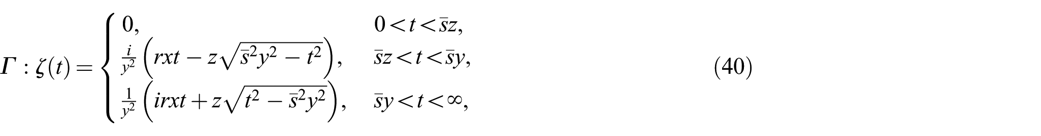
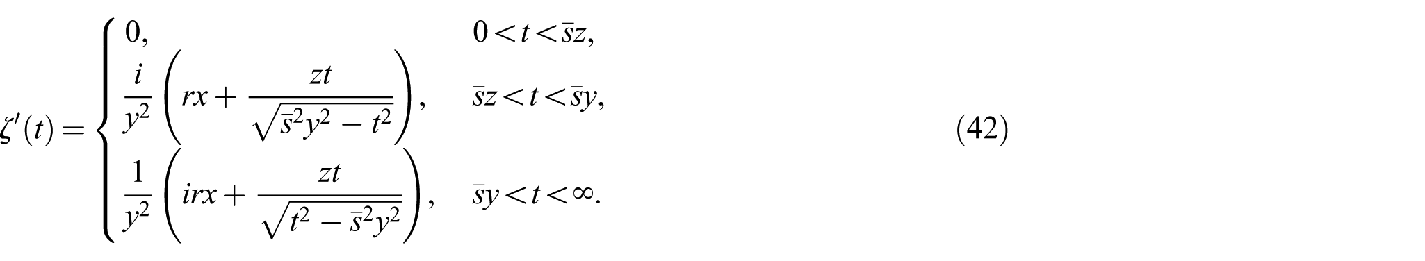
ζ = \frac{irxt \pm z \sqrt{t^{2} - {\bar{s}}^{2} (r^{2} x^{2} + z^{2})}}{r^{2} x^{2} + z^{2}} .

(39)

The above solutions, for given $r, z$ and x, can be regarded as parametric representations for two curves in the complex $ζ$ plane as the parameter t varies on the positive part of the real line. In particular, a path, namely $Γ$ , can be defined in this manner by the piecewise parametric representation as

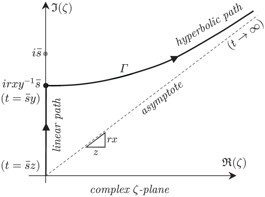
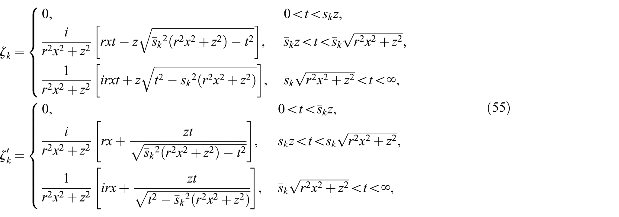
Γ : ζ (t) = {\begin{matrix} 0, & 0 < t < \bar{s} z, \\ \frac{i}{y^{2}} (rxt - z \sqrt{{\bar{s}}^{2} y^{2} - t^{2}}), & \bar{s} z < t < \bar{s} y, \\ \frac{1}{y^{2}} (irxt + z \sqrt{t^{2} - {\bar{s}}^{2} y^{2}}), & \bar{s} y < t < \infty, \end{matrix}

(40)

where $y = \sqrt{r^{2} x^{2} + z^{2}}$ is an auxiliary variable that will be used, merely, for brevity of expressions. As shown schematically in Figure 3, the path $Γ$ is stationary on $ζ = 0$ for $0 < t < \bar{s} z$ . Then, it traces a linear segment on the positive $ℑ (ζ)$ -axis from $ζ = 0$ to $ζ = irx y^{- 1} \bar{s}$ for $\bar{s} z < t < \bar{s} y$ . Afterwards, it traces a hyperbolic curve from $ζ = irx y^{- 1} \bar{s}$ to $ζ = \infty$ in the first quadrant of the complex $ζ$ -plane as the parameter t changes in the interval $\bar{s} y < t < \infty .$ It is worth mentioning that since $rx y^{- 1} \bar{s} < \bar{s}$ for all r and z and all $x \geq 1$ , the path $Γ$ never encounters the point $ζ = i \bar{s}$ , as illustrated in Figure 3.

Figure 3.

Schematic illustration of the path $Γ$ . The path is composed of a linear segment on the positive imaginary axis and a hyperbolic semi-branch.

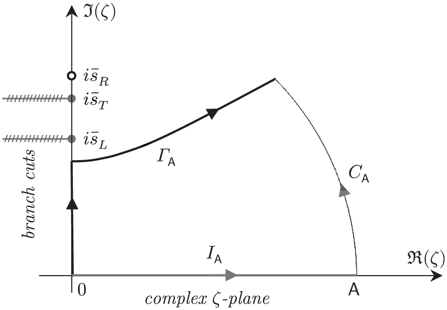
We now consider the inner integral in equation (37). Obviously, this integral can be understood as an integral on the positive $ℜ (ζ)$ -axis in the complex $ζ$ -plane. Since $g (ζ)$ is assumed to contain the radicals $α$ and $β$ , for complex $ζ$ this function is rendered multivalued and thus ambiguous. To prevent this, one has to introduce branch cuts emanating from the branch points $ζ = \pm i {\bar{s}}_{L}, \pm i {\bar{s}}_{T}$ , as illustrated in Figure 4. In this figure, only the branch points in the upper half-plane are depicted. Moreover, the function $g (ζ)$ is allowed to have poles or other singularities as long as they are positioned outside the first quadrant of the complex $ζ$ -plane and such that they do not interfere with the path $Γ$ , as it is the case encountered here. In this problem $g (ζ)$ has simple poles at $ζ = \pm i {\bar{s}}_{R}$ , where ${\bar{s}}_{R}$ denotes the slowness of Rayleigh waves [2]). Yet, this brings no concern here as the inequality ${\bar{s}}_{L} < {\bar{s}}_{T} < {\bar{s}}_{R}$ (see [2]) ensures that the path $Γ$ stays clear of the poles.

Figure 4.

Integration paths and the branch cuts. ${\bar{s}}_{L}$ , ${\bar{s}}_{T}$ and ${\bar{s}}_{R}$ are the slowness constants for longitudinal, transverse and Rayleigh wavefronts, respectively.

As depicted in Figure 4, we now seek to alter the integration path for the inner integral in equation (37) from the $ℜ (ζ)$ -axis to the path $Γ$ (on which t is real and positive) by the aid of a circular arc $C_{A}$ that starts from the point A on the $ℜ (ζ)$ -axis and intersects with $Γ$ to form the finite path $Γ Φ_{A}$ . The integrand inside the closed contour $I_{A} \cup C_{A} \cup Γ_{A}^{-}$ is analytic, where $Γ_{A}^{-}$ denotes the path $Γ Φ_{A}$ traced in the reversed direction. Hence, knowing that the integral on $C_{A}$ vanishes as $A \to \infty$ (since the integrand contains a factor $e^{- sz γ}$ that diminishes exponentially as $| ζ | = A$ is increased), one may write

\int_{0}^{\infty} ζ g (ζ) e^{- st} d ζ = \int_{Γ} ζ g (ζ) e^{- st} d ζ = \int_{0}^{\infty} ζ (t) ζ' (t) g (ζ (t)) e^{- st} dt,

(41)

by Cauchy’s integral theorem [32], where $ζ (t)$ is given by equation (40), and $ζ' (t)$ denotes its time derivative, i.e.

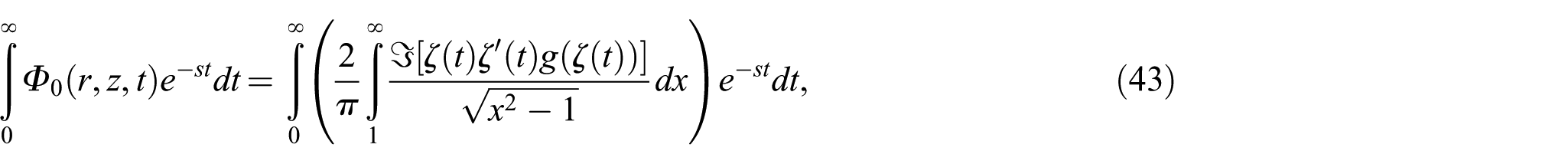
ζ' (t) = {\begin{matrix} 0, & 0 < t < \bar{s} z, \\ \frac{i}{y^{2}} (rx + \frac{zt}{\sqrt{{\bar{s}}^{2} y^{2} - t^{2}}}), & \bar{s} z < t < \bar{s} y, \\ \frac{1}{y^{2}} (irx + \frac{zt}{\sqrt{t^{2} - {\bar{s}}^{2} y^{2}}}), & \bar{s} y < t < \infty . \end{matrix}

(42)

Now, combining the equations (37) and (41) and changing the order of integration again results in

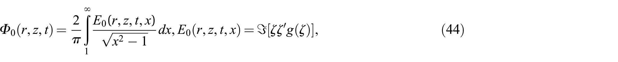
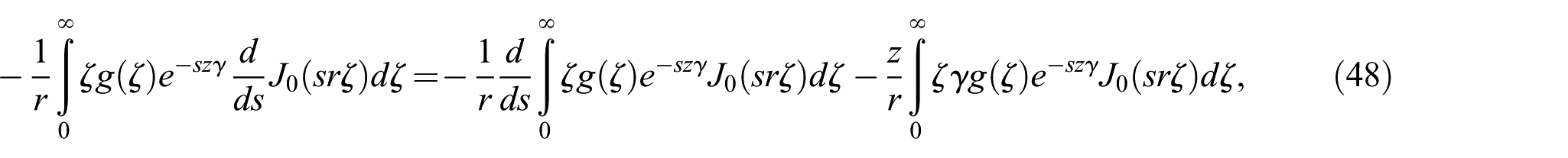
\int_{0}^{\infty} Φ_{0} (r, z, t) e^{- st} dt = \int_{0}^{\infty} (\frac{2}{π} \int_{1}^{\infty} \frac{ℑ [ζ (t) ζ' (t) g (ζ (t))]}{\sqrt{x^{2} - 1}} dx) e^{- st} dt,

(43)

from which the solution of the integral equation (35) follows immediately in view of the uniqueness theorem for Laplace transforms [13] as

Φ_{0} (r, z, t) = \frac{2}{π} \int_{1}^{\infty} \frac{E_{0} (r, z, t, x)}{\sqrt{x^{2} - 1}} dx, E_{0} (r, z, t, x) = ℑ [ζ ζ' g (ζ)],

(44)

where $ζ$ and $ζ'$ are given by equations (40) and (42), respectively.

4.6. Inverse Laplace transform of EIs of orders $ν = 1$ and 2

The well-known recursion formulae for Bessel functions [31]

\frac{d}{dx} [x^{ν} J_{ν} (x)] = x^{ν} J_{ν - 1} (x), J_{ν - 1} (x) + J_{ν + 1} (x) = \frac{2 ν}{x} J_{ν} (x),

(45)

enable us to write

J_{1} (sr ζ) = - \frac{1}{r ζ} \frac{d}{ds} J_{0} (sr ζ), J_{2} (sr ζ) = J_{0} (sr ζ) + \frac{2}{r^{2} ζ^{2}} \frac{d^{2}}{d s^{2}} J_{0} (sr ζ) .

(46)

For the case $ν = 1$ , the Laplace transform inversion of equation (34) takes the form of the integral equation

\int_{0}^{\infty} Φ_{1} (r, z, t) e^{- st} dt = \int_{0}^{\infty} ζ^{2} g (ζ) e^{- sz γ} J_{1} (sr ζ) d ζ, γ = \sqrt{ζ^{2} + s^{2}},

(47)

for $Φ_{1} (r, z, t)$ . Using the first formula in equations (46), the right-hand side of equation (47) can be converted into

- \frac{1}{r} \int_{0}^{\infty} ζ g (ζ) e^{- sz γ} \frac{d}{ds} J_{0} (sr ζ) d ζ = - \frac{1}{r} \frac{d}{ds} \int_{0}^{\infty} ζ g (ζ) e^{- sz γ} J_{0} (sr ζ) d ζ - \frac{z}{r} \int_{0}^{\infty} ζ γ g (ζ) e^{- sz γ} J_{0} (sr ζ) d ζ,

(48)

as two integrals, both of which have the form of an EI of order $ν = 0$ . By using the properties of Laplace transforms [13] and the solution in equation (44), it can be inferred that the solution for the integral equation (47) is

Φ_{1} (r, z, t) = \frac{2}{π} \int_{1}^{\infty} \frac{E_{1} (r, z, t, x)}{\sqrt{x^{2} - 1}} dx, E_{1} (r, z, t, x) = ℑ [ζ ζ' g (ζ) (\frac{t}{r} - \frac{z}{r} \sqrt{ζ^{2} + {\bar{s}}^{2}})],

(49)

with $ζ$ and $ζ'$ as given by equations (40) and (42), respectively. Similarly, for the case $ν = 2$ , the Laplace transform inversion of equation (34) leads to the solution of the integral equation

\int_{0}^{\infty} Φ_{2} (r, z, t) e^{- st} dt = \int_{0}^{\infty} ζ^{3} g (ζ) e^{- sz γ} J_{2} (sr ζ) d ζ, γ = \sqrt{ζ^{2} + {\bar{s}}^{2}},

(50)

for $Φ_{2} (r, z, t)$ . Now, by utilising the second formula in equation (46) for $J_{2} (sr ζ)$ and following a similar procedure employed for the case $ν = 1$ , the solution of the integral equation (50) can be found as

\begin{matrix} Φ_{2} (r, z, t) = \frac{2}{π} \int_{1}^{\infty} \frac{E_{2} (r, z, t, x)}{\sqrt{x^{2} - 1}} dx, \\ E_{2} (r, z, t, x) = ℑ [ζ ζ' g (ζ) (ζ^{2} + \frac{2 t^{2}}{r^{2}} - \frac{4 zt}{r^{2}} \sqrt{ζ^{2} + {\bar{s}}^{2}} + \frac{2 z^{2}}{r^{2}} (ζ^{2} + {\bar{s}}^{2}))], \end{matrix}

(51)

where $ζ$ and $ζ'$ are given in equations (40) and (42), as usual. It might be of interest to make use of equation (38) in the solutions in equations (44), (49) and (51). Namely, from equation (38) one has the relation $z γ = t + irx ζ$ which can be used to simplify the solutions. This leads to alternate, but entirely equivalent forms for these formulae.

4.7. Time-domain displacement components

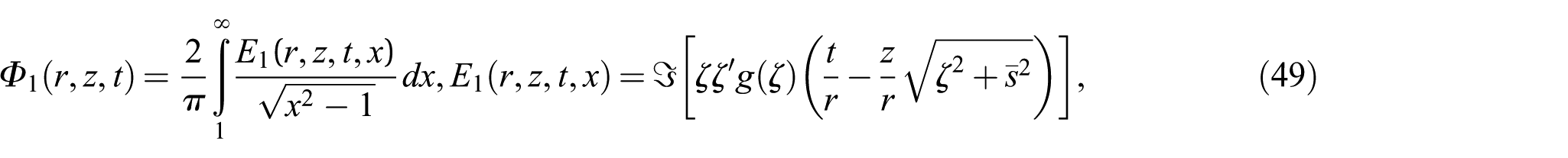
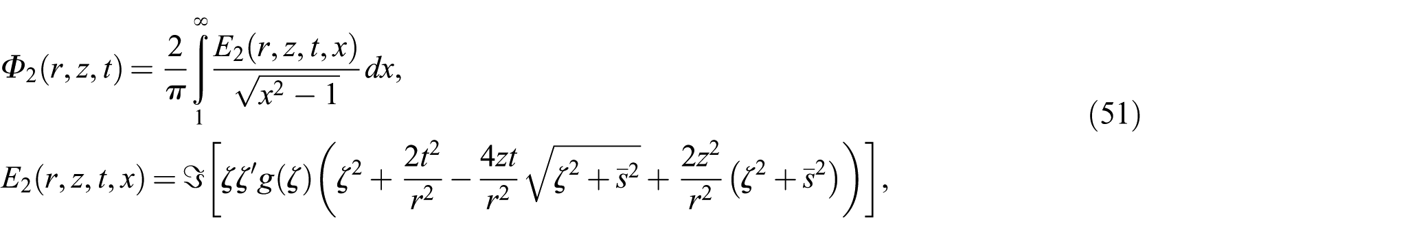
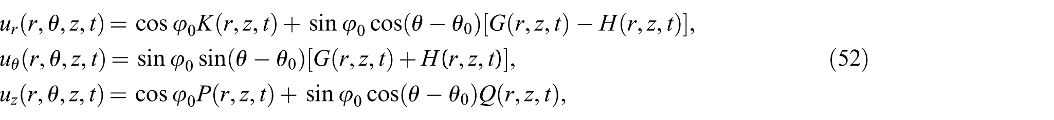
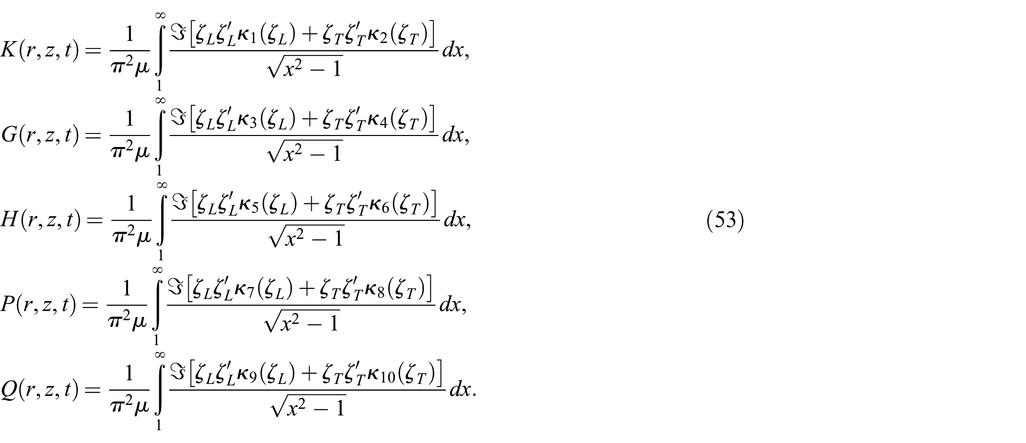
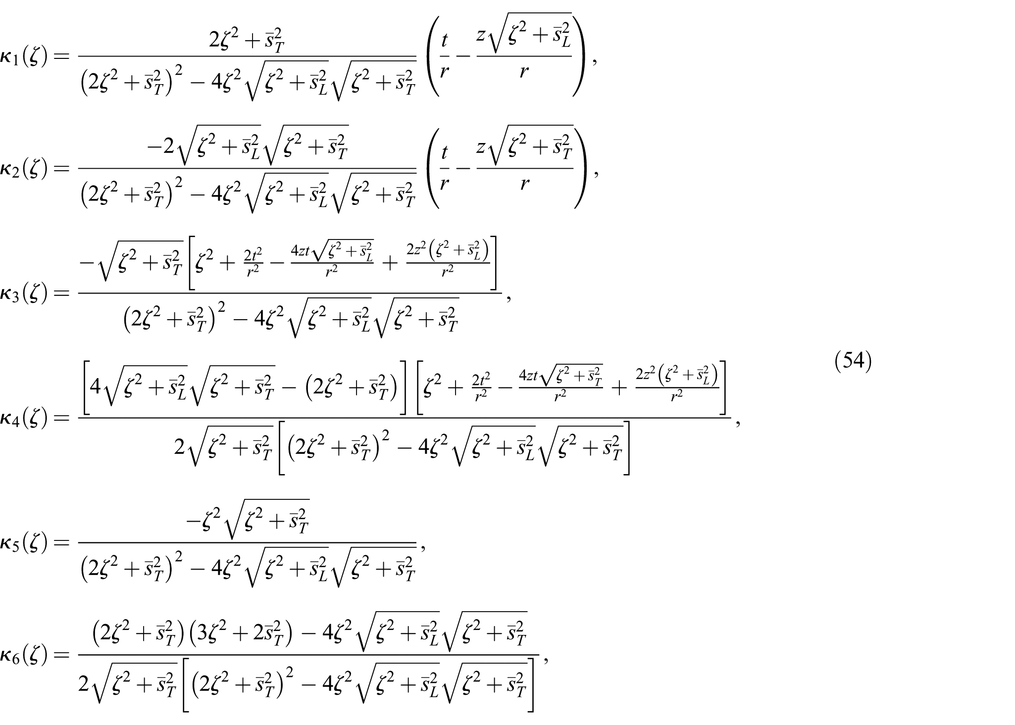
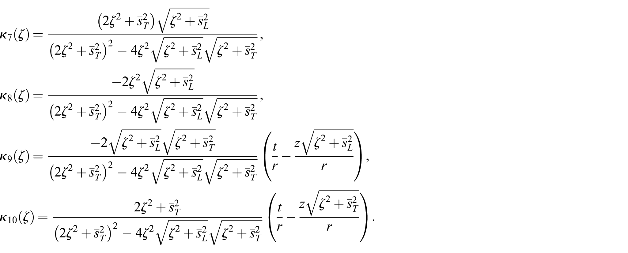
Having found a method for Laplace transform inversion for EIs, all the ingredients are ready for an easy acquisition of the inverse Laplace transform of the integrals given in equation (33). Consequently, the complete set of final solutions of the initial boundary value problem defined in Section 2 may be written out explicitly as

\begin{matrix} u_{r} (r, θ, z, t) = \cos φ_{0} K (r, z, t) + \sin φ_{0} \cos (θ - θ_{0}) [G (r, z, t) - H (r, z, t)], \\ u_{θ} (r, θ, z, t) = \sin φ_{0} \sin (θ - θ_{0}) [G (r, z, t) + H (r, z, t)], \\ u_{z} (r, θ, z, t) = \cos φ_{0} P (r, z, t) + \sin φ_{0} \cos (θ - θ_{0}) Q (r, z, t), \end{matrix}

(52)

in which

\begin{matrix} K (r, z, t) = \frac{1}{π^{2} μ} \int_{1}^{\infty} \frac{ℑ [ζ_{L} ζ_{L}' κ_{1} (ζ_{L}) + ζ_{T} ζ_{T}' κ_{2} (ζ_{T})]}{\sqrt{x^{2} - 1}} dx, \\ G (r, z, t) = \frac{1}{π^{2} μ} \int_{1}^{\infty} \frac{ℑ [ζ_{L} ζ_{L}' κ_{3} (ζ_{L}) + ζ_{T} ζ_{T}' κ_{4} (ζ_{T})]}{\sqrt{x^{2} - 1}} dx, \\ H (r, z, t) = \frac{1}{π^{2} μ} \int_{1}^{\infty} \frac{ℑ [ζ_{L} ζ_{L}' κ_{5} (ζ_{L}) + ζ_{T} ζ_{T}' κ_{6} (ζ_{T})]}{\sqrt{x^{2} - 1}} dx, \\ P (r, z, t) = \frac{1}{π^{2} μ} \int_{1}^{\infty} \frac{ℑ [ζ_{L} ζ_{L}' κ_{7} (ζ_{L}) + ζ_{T} ζ_{T}' κ_{8} (ζ_{T})]}{\sqrt{x^{2} - 1}} dx, \\ Q (r, z, t) = \frac{1}{π^{2} μ} \int_{1}^{\infty} \frac{ℑ [ζ_{L} ζ_{L}' κ_{9} (ζ_{L}) + ζ_{T} ζ_{T}' κ_{10} (ζ_{T})]}{\sqrt{x^{2} - 1}} dx . \end{matrix}

(53)

and

\begin{matrix} κ_{1} (ζ) = \frac{2 ζ^{2} + {\bar{s}}_{T}^{2}}{{(2 ζ^{2} + {\bar{s}}_{T}^{2})}^{2} - 4 ζ^{2} \sqrt{ζ^{2} + {\bar{s}}_{L}^{2}} \sqrt{ζ^{2} + {\bar{s}}_{T}^{2}}} (\frac{t}{r} - \frac{z \sqrt{ζ^{2} + {\bar{s}}_{L}^{2}}}{r}), \\ κ_{2} (ζ) = \frac{- 2 \sqrt{ζ^{2} + {\bar{s}}_{L}^{2}} \sqrt{ζ^{2} + {\bar{s}}_{T}^{2}}}{{(2 ζ^{2} + {\bar{s}}_{T}^{2})}^{2} - 4 ζ^{2} \sqrt{ζ^{2} + {\bar{s}}_{L}^{2}} \sqrt{ζ^{2} + {\bar{s}}_{T}^{2}}} (\frac{t}{r} - \frac{z \sqrt{ζ^{2} + {\bar{s}}_{T}^{2}}}{r}), \\ κ_{3} (ζ) = \frac{- \sqrt{ζ^{2} + {\bar{s}}_{T}^{2}} [ζ^{2} + \frac{2 t^{2}}{r^{2}} - \frac{4 zt \sqrt{ζ^{2} + {\bar{s}}_{L}^{2}}}{r^{2}} + \frac{2 z^{2} (ζ^{2} + {\bar{s}}_{L}^{2})}{r^{2}}]}{{(2 ζ^{2} + {\bar{s}}_{T}^{2})}^{2} - 4 ζ^{2} \sqrt{ζ^{2} + {\bar{s}}_{L}^{2}} \sqrt{ζ^{2} + {\bar{s}}_{T}^{2}}}, \\ κ_{4} (ζ) = \frac{[4 \sqrt{ζ^{2} + {\bar{s}}_{L}^{2}} \sqrt{ζ^{2} + {\bar{s}}_{T}^{2}} - (2 ζ^{2} + {\bar{s}}_{T}^{2})] [ζ^{2} + \frac{2 t^{2}}{r^{2}} - \frac{4 zt \sqrt{ζ^{2} + {\bar{s}}_{T}^{2}}}{r^{2}} + \frac{2 z^{2} (ζ^{2} + {\bar{s}}_{L}^{2})}{r^{2}}]}{2 \sqrt{ζ^{2} + {\bar{s}}_{T}^{2}} [{(2 ζ^{2} + {\bar{s}}_{T}^{2})}^{2} - 4 ζ^{2} \sqrt{ζ^{2} + {\bar{s}}_{L}^{2}} \sqrt{ζ^{2} + {\bar{s}}_{T}^{2}}]}, \\ κ_{5} (ζ) = \frac{- ζ^{2} \sqrt{ζ^{2} + {\bar{s}}_{T}^{2}}}{{(2 ζ^{2} + {\bar{s}}_{T}^{2})}^{2} - 4 ζ^{2} \sqrt{ζ^{2} + {\bar{s}}_{L}^{2}} \sqrt{ζ^{2} + {\bar{s}}_{T}^{2}}}, \\ κ_{6} (ζ) = \frac{(2 ζ^{2} + {\bar{s}}_{T}^{2}) (3 ζ^{2} + 2 {\bar{s}}_{T}^{2}) - 4 ζ^{2} \sqrt{ζ^{2} + {\bar{s}}_{L}^{2}} \sqrt{ζ^{2} + {\bar{s}}_{T}^{2}}}{2 \sqrt{ζ^{2} + {\bar{s}}_{T}^{2}} [{(2 ζ^{2} + {\bar{s}}_{T}^{2})}^{2} - 4 ζ^{2} \sqrt{ζ^{2} + {\bar{s}}_{L}^{2}} \sqrt{ζ^{2} + {\bar{s}}_{T}^{2}}]}, \end{matrix}

(54)

\begin{matrix} κ_{7} (ζ) = \frac{(2 ζ^{2} + {\bar{s}}_{T}^{2}) \sqrt{ζ^{2} + {\bar{s}}_{L}^{2}}}{{(2 ζ^{2} + {\bar{s}}_{T}^{2})}^{2} - 4 ζ^{2} \sqrt{ζ^{2} + {\bar{s}}_{L}^{2}} \sqrt{ζ^{2} + {\bar{s}}_{T}^{2}}}, \\ κ_{8} (ζ) = \frac{- 2 ζ^{2} \sqrt{ζ^{2} + {\bar{s}}_{L}^{2}}}{{(2 ζ^{2} + {\bar{s}}_{T}^{2})}^{2} - 4 ζ^{2} \sqrt{ζ^{2} + {\bar{s}}_{L}^{2}} \sqrt{ζ^{2} + {\bar{s}}_{T}^{2}}}, \\ κ_{9} (ζ) = \frac{- 2 \sqrt{ζ^{2} + {\bar{s}}_{L}^{2}} \sqrt{ζ^{2} + {\bar{s}}_{T}^{2}}}{{(2 ζ^{2} + {\bar{s}}_{T}^{2})}^{2} - 4 ζ^{2} \sqrt{ζ^{2} + {\bar{s}}_{L}^{2}} \sqrt{ζ^{2} + {\bar{s}}_{T}^{2}}} (\frac{t}{r} - \frac{z \sqrt{ζ^{2} + {\bar{s}}_{L}^{2}}}{r}), \\ κ_{10} (ζ) = \frac{2 ζ^{2} + {\bar{s}}_{T}^{2}}{{(2 ζ^{2} + {\bar{s}}_{T}^{2})}^{2} - 4 ζ^{2} \sqrt{ζ^{2} + {\bar{s}}_{L}^{2}} \sqrt{ζ^{2} + {\bar{s}}_{T}^{2}}} (\frac{t}{r} - \frac{z \sqrt{ζ^{2} + {\bar{s}}_{T}^{2}}}{r}) . \end{matrix}

In the formulae of equation (53), $ζ_{L}$ , $ζ_{L}'$ , $ζ_{T}$ and $ζ_{T}'$ are piecewise complex-valued functions of four real variables r, $z,$ t and x defined as

\begin{matrix} ζ_{k} = {\begin{matrix} 0, & 0 < t < {\bar{s}}_{k} z, \\ \frac{i}{r^{2} x^{2} + z^{2}} [rxt - z \sqrt{{\bar{s}}_{k}^{2} (r^{2} x^{2} + z^{2}) - t^{2}}], & {\bar{s}}_{k} z < t < {\bar{s}}_{k} \sqrt{r^{2} x^{2} + z^{2}}, \\ \frac{1}{r^{2} x^{2} + z^{2}} [irxt + z \sqrt{t^{2} - {\bar{s}}_{k}^{2} (r^{2} x^{2} + z^{2})}], & {\bar{s}}_{k} \sqrt{r^{2} x^{2} + z^{2}} < t < \infty, \end{matrix} \\ ζ_{k}' = {\begin{matrix} 0, & 0 < t < {\bar{s}}_{k} z, \\ \frac{i}{r^{2} x^{2} + z^{2}} [rx + \frac{zt}{\sqrt{{\bar{s}}_{k}^{2} (r^{2} x^{2} + z^{2}) - t^{2}}}], & {\bar{s}}_{k} z < t < {\bar{s}}_{k} \sqrt{r^{2} x^{2} + z^{2}}, \\ \frac{1}{r^{2} x^{2} + z^{2}} [irx + \frac{zt}{\sqrt{t^{2} - {\bar{s}}_{k}^{2} (r^{2} x^{2} + z^{2})}}], & {\bar{s}}_{k} \sqrt{r^{2} x^{2} + z^{2}} < t < \infty, \end{matrix} \end{matrix}

(55)

where the index k is either L or T.

Indeed, with the notions previously introduced, $ζ = ζ_{L} (t)$ and $ζ = ζ_{T} (t)$ are parametric representations for paths of integration $Γ Φ_{L}$ and $Γ Φ_{T}$ in the complex $ζ$ -plane that are used in the Laplace transform inversion process of EIs corresponding to longitudinal and transverse waves, respectively. These two paths are represented in Figures 5 and 6. It can be shown that the linear part of $Γ Φ_{T}$ does encounter the branch point $ζ = i {\bar{s}}_{L}$ on the $ℑ (ζ)$ -axis. For circumventing this issue, a semicircular indentation with vanishing radius is made on the path $Γ Φ_{T}$ (shown schematically in Figure 6). It can be proven, nonetheless, that this indentation does not contribute to the integrals [2], and hence the above solutions remain valid. The set of solutions given herein by the equations (52)–(55) are valid for all $r, z, t > 0$ , $- \infty < θ < \infty$ , and they can be used for the evaluation of the transient motions in a half-space with arbitrary $λ$ and $μ$ .

Figure 5.

Schematic illustration of the path $Γ_{L}$ for longitudinal wavefronts. As the ratio $z / r$ is decreased, the slope of the asymptote is increased.

Figure 6.

Schematic illustration of the path $Γ_{T}$ for transverse wavefronts. As the ratio $z / r$ is decreased, the slope of the asymptote is increased.

The solutions for $r = 0$ and $z > 0$ may be obtained by fixing $r = 0$ . In that case, a quick reference to equation (33) shows that all the integrals except $\tilde{H}$ and $\tilde{P}$ vanish, inside which the function $J_{0} (sr ζ)$ will be further reduced to unity for $r = 0$ . Hence, the parameter s will only appear in the factors $e^{- sz γ}$ , with $γ = α$ or $β$ . The Laplace transform inversion for this special case can be carried out easily via the change of variable $t = z γ$ , as suggested by equation (38) for $r = 0$ . Indeed, with this change of variables, t will be real and positive without the any need for integration path alterations, and the solutions can be obtained in closed-form, which coincide with the solutions given in [5] and [14].

The solutions on the boundary $\partial Ω$ ( $r > 0$ and $z = 0$ ) may be found by letting z approach zero. In that case, the EI of equation (34) will be reduced to a simpler one excluding the factor $e^{- sz γ}$ in the integrands, which can be handled by making the change of variable $t = - irx ζ$ in the course of Laplace transform inversion, as suggested by equation (38) for $z = 0$ . Then, a purely imaginary $ζ$ with $ℑ (ζ) > 0$ will result in a real and positive t, as desired. Therefore, altering the path of integration from the positive $ℜ (ζ)$ -axis to the positive $ℑ (ζ)$ -axis (with the necessary indentations around the singular points) will lead to the time-domain solutions exactly the same as the solutions reported in [7] and [12]. The path alteration to the positive $ℑ (ζ)$ -axis, as needed for surface solutions, is also confirmed by referring to Figures 5 and 6. When $z \to 0$ , the slope of the asymptote of the hyperbolic parts of the paths $Γ Φ_{L}$ and $Γ Φ_{T}$ tends to infinity, which leads to the ideal linear paths along the positive $ℑ (ζ)$ -axis, as shown schematically by grey, dotted paths in these figures. Since the solutions for the cases $r = 0$ , $z > 0$ and $r > 0$ , $z = 0$ have been fully presented in a recent work [14], they are not repeated herein. We have instead focused on the extension of the previously found solutions of Lamb’s problem for the case $r, z > 0$ .

Due to the solution method pursued in this paper, the solution formulae in equations (52)–(55) are presented in much more elegant and compact forms as compared to the previous studies. Obviously terms including the functions $ζ_{L}$ and $ζ_{T}$ in equations (53) correspond to the contributions of longitudinal and transverse wavefronts (P-wave and S-wave, respectively, in seismological terminology) in the final elastodynamic displacement field. However, at the first glance it might seem difficult to separate the contributions of the wave motions that are of mixed P and S origin (such as Rayleigh waves and head waves), should such physical interpretations of the mathematical formulae be needed. For that purpose, one needs to expand equations (52)–(55) and meticulously analyse all the terms. For example, the numerators of the integrands of the integrals of equation (53) are imaginary parts of some rather complicated complex-valued functions given by equations (54) and (55). Simplifying the imaginary parts of the mentioned functions will then lead to integrals in equivalent real forms in which the different aspects of wave propagation phenomena can be more readily separated. It is emphasised, nevertheless, that the solution formulae of equations (52)–(55) are complete and computationally effective in their current compact forms.

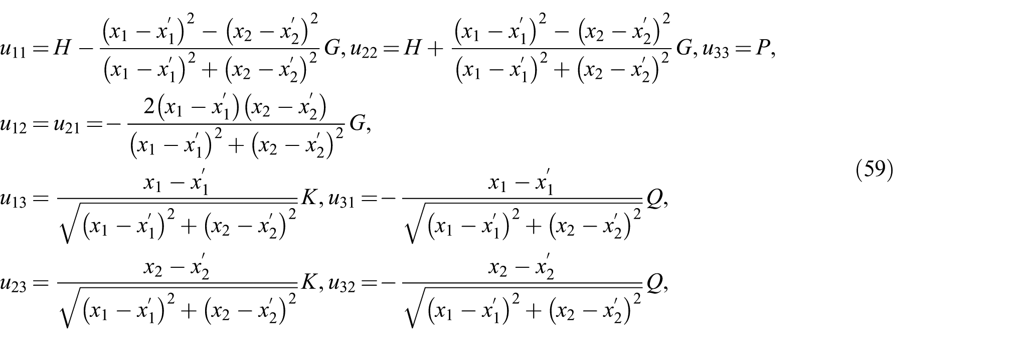
4.8. Time-domain displacement Green’s functions in Cartesian coordinate system

For many applications (e.g. the boundary element methods [33]), it is useful to express the solutions of equations (52)–(55) in the form of Green’s functions. Here, we obtain the time-domain Green’s functions for Lamb’s problem from the already found interior solutions. For that purpose, using of the coordinate transformation formulae $x_{1} = r \cos θ$ , $x_{2} = r \sin θ$ and $x_{3} = z$ , and trigonometric identities, we find from equation (52) that

\begin{matrix} u_{1} = \cos φ_{0} \cos θ K + \sin φ_{0} \cos (2 θ - θ_{0}) G - \sin φ_{0} \cos θ_{0} H, \\ u_{2} = \cos φ_{0} \sin θ K + \sin φ_{0} \sin (2 θ - θ_{0}) G - \sin φ_{0} \sin θ_{0} H, \\ u_{3} = \cos φ_{0} P + \sin φ_{0} \cos (θ - θ_{0}) Q, \end{matrix}

(56)

where the functions $u_{j}$ ( $j = 1, 2, 3$ ), denote the displacement components in the Cartesian coordinates. Moreover, according to Figure 2, fixing the ordered pair $(φ_{0}, θ_{0})$ as $(π / 2, π)$ , $(π / 2, 3 π / 2)$ and $(0, θ_{0})$ corresponds to the point load being applied in the positive directions of $x_{1}$ , $x_{2}$ and $x_{3}$ axes, respectively. Substituting these values of $φ_{0}$ and $θ_{0}$ in equation (56), one finds

\begin{matrix} u_{11} = H - G \cos 2 θ, u_{12} = - G \sin 2 θ, u_{13} = K \cos θ, \\ u_{21} = - G \sin 2 θ, u_{22} = H + G \cos 2 θ, u_{23} = K \sin θ, \\ u_{31} = - Q \cos θ, u_{32} = - Q \sin θ, u_{33} = P, \end{matrix}

(57)

in which $u_{jk}$ , ( $j, k = 1, 2, 3$ ), represents the displacement in the direction of $x_{j}$ -axis due to a surface point load being applied at the origin in the direction of $x_{k}$ -axis. In the context of Green’s functions, it is also desirable to remove the restriction of the location of the surface point load p , which is fixed as the origin (see Figures 1 and 2). Since the medium is homogeneous, this can be achieved easily by translating the Cartesian coordinate system in the $x_{1} x_{2}$ -plane from the origin to an arbitrary point $(- x_{1}', - x_{2}', 0)$ . With this translation, we shall have the coordinate transformation formulae

r = \sqrt{{(x_{1} - x_{1}^{'})}^{2} + {(x_{2} - x_{2}^{'})}^{2}}, θ = \tan^{- 1} (\frac{x_{2} - x_{2}^{'}}{x_{1} - x_{1}^{'}}), z = x_{3},

(58)

that relate the original cylindrical coordinates $(r, θ, z)$ , see Figure 1, to the new translated Cartesian coordinates $(x_{1}, x_{2}, x_{3})$ , and by which the equations (57) can be finally expressed as

\begin{matrix} u_{11} = H - \frac{{(x_{1} - x_{1}^{'})}^{2} - {(x_{2} - x_{2}^{'})}^{2}}{{(x_{1} - x_{1}^{'})}^{2} + {(x_{2} - x_{2}^{'})}^{2}} G, u_{22} = H + \frac{{(x_{1} - x_{1}^{'})}^{2} - {(x_{2} - x_{2}^{'})}^{2}}{{(x_{1} - x_{1}^{'})}^{2} + {(x_{2} - x_{2}^{'})}^{2}} G, u_{33} = P, \\ u_{12} = u_{21} = - \frac{2 (x_{1} - x_{1}^{'}) (x_{2} - x_{2}^{'})}{{(x_{1} - x_{1}^{'})}^{2} + {(x_{2} - x_{2}^{'})}^{2}} G, \\ u_{13} = \frac{x_{1} - x_{1}^{'}}{\sqrt{{(x_{1} - x_{1}^{'})}^{2} + {(x_{2} - x_{2}^{'})}^{2}}} K, u_{31} = - \frac{x_{1} - x_{1}^{'}}{\sqrt{{(x_{1} - x_{1}^{'})}^{2} + {(x_{2} - x_{2}^{'})}^{2}}} Q, \\ u_{23} = \frac{x_{2} - x_{2}^{'}}{\sqrt{{(x_{1} - x_{1}^{'})}^{2} + {(x_{2} - x_{2}^{'})}^{2}}} K, u_{32} = - \frac{x_{2} - x_{2}^{'}}{\sqrt{{(x_{1} - x_{1}^{'})}^{2} + {(x_{2} - x_{2}^{'})}^{2}}} Q, \end{matrix}

(59)

where one has to transmute r and z in accordance with equation (58) in the integrals $K, \dots, Q$ given previously by the equations (53)–(55). The functions $u_{jk} = u_{jk} (x_{1}, x_{2}, x_{3}, t; x_{1}', x_{2}', 0)$ acquired as above represent the time-domain elastodynamic Green’s functions for a homogeneous, isotropic half-space due to an impulsive point source located at $(x_{1}', x_{2}', 0)$ and varying with time as the Heaviside unit step function.

4.9. Solutions for infinite time: the classical Boussinesq–Cerruti solutions

Since the time dependence $p (t)$ of the dynamical point load has been chosen in the foregoing analysis to be the Heaviside unit step function, one may intuitively expect that for sufficiently large values of time, once the ephemeral tremors have been attenuated, the displacement components shall approach to certain time-independent values, equivalent to those obtained in elastostatics. This proposition may be corroborated by referring to the time-history diagrams of displacements, as shown in the next section. More elegantly though, closed-form expressions can be found for these limiting solutions. Therefore, as it might be of theoretical interest, we investigate the elastodynamic solutions in equation (52) for the limit case $t \to \infty$ . For that purpose, we use the final value theorem

lim_{t \to \infty} f (r, θ, z, t) = lim_{s \to 0} [s \tilde{f} (r, θ, z, s)],

(60)

for a typical function f provided that the limit of this function exists as $t \to \infty$ , as verified by using the properties of the Laplace transforms [13]. The limits of the displacement components of equation (52) shall be determined by finding the limits of the integrals in equation (53), i.e.

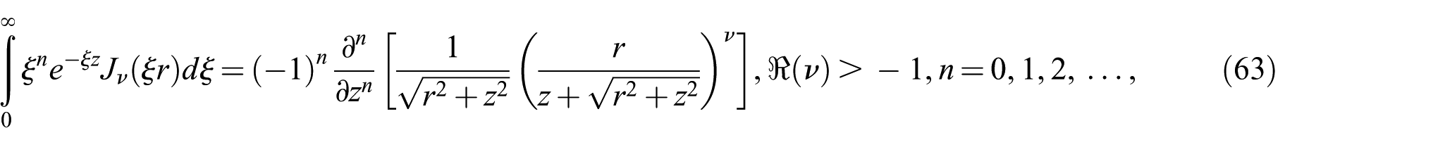
\begin{matrix} u_{r}^{st} (r, θ, z) = \cos φ_{0} K^{st} (r, z) + \sin φ_{0} \cos (θ - θ_{0}) [G^{st} (r, z) - H^{st} (r, z)], \\ u_{θ}^{st} (r, θ, z) = \sin φ_{0} \sin (θ - θ_{0}) [G^{st} (r, z) + H^{st} (r, z)], \\ u_{z}^{st} (r, θ, z) = \cos φ_{0} P^{st} (r, z) + \sin φ_{0} \cos (θ - θ_{0}) Q^{st} (r, z), \end{matrix}

(61)

where the superscript st denotes the limits of the corresponding function as $t \to \infty$ . Finding the functions $K^{st}, \dots, Q^{st}$ in turn, is facilitated by making use of equation (60) in the equations (31) and recalling that $\tilde{p} (s) = s^{- 1}$ for the point load with Heaviside time dependence. Subsequently, one has to deal with the limits of integrals given in equation (31) as $s \to 0$ . Assuming that interchanging of the order of limits and integrals is justified, one may use L’Hôpital’s rule to find ultimately

\begin{matrix} K^{st} (r, z) = \frac{1}{4 π μ} \int_{0}^{\infty} (ξ z - \frac{μ}{λ + μ}) e^{- ξ z} J_{1} (ξ r) d ξ = \frac{1}{4 π μ} [\frac{rz}{{(r^{2} + z^{2})}^{\frac{3}{2}}} + \frac{μ}{λ + μ} (\frac{z}{r \sqrt{r^{2} + z^{2}}} - \frac{1}{r})], \\ G^{st} (r, z) = \frac{- 1}{8 π μ} \int_{0}^{\infty} (ξ z + \frac{λ}{λ + μ}) e^{- ξ z} J_{2} (ξ r) d ξ = \frac{- r^{2}}{8 π μ} [\frac{(z^{2} + 2 z \sqrt{r^{2} + z^{2}}) + (\frac{λ}{λ + μ}) (r^{2} + z^{2})}{{(r^{2} + z^{2})}^{\frac{3}{2}} {(z + \sqrt{r^{2} + z^{2}})}^{2}}], \\ H^{st} (r, z) = \frac{- 1}{8 π μ} \int_{0}^{\infty} (ξ z - \frac{3 λ + 4 μ}{λ + μ}) e^{- ξ z} J_{0} (ξ r) d ξ = \frac{- 1}{8 π μ} [\frac{z^{2}}{{(r^{2} + z^{2})}^{\frac{3}{2}}} - (\frac{3 λ + 4 μ}{λ + μ}) \frac{1}{\sqrt{r^{2} + z^{2}}}], \\ P^{st} (r, z) = \frac{1}{4 π μ} \int_{0}^{\infty} (ξ z + \frac{λ + 2 μ}{λ + μ}) e^{- ξ z} J_{0} (ξ r) d ξ = \frac{1}{4 π μ} [\frac{z^{2}}{{(r^{2} + z^{2})}^{\frac{3}{2}}} + (\frac{λ + 2 μ}{λ + μ}) \frac{1}{\sqrt{r^{2} + z^{2}}}], \\ Q^{st} (r, z) = \frac{- 1}{4 π μ} \int_{0}^{\infty} (ξ z + \frac{μ}{λ + μ}) e^{- ξ z} J_{1} (ξ r) d ξ = \frac{1}{4 π μ} [\frac{μ}{λ + μ} (\frac{z}{r \sqrt{r^{2} + z^{2}}} - \frac{1}{r}) - \frac{rz}{{(r^{2} + z^{2})}^{\frac{3}{2}}}], \end{matrix}

(62)

where the formula [31]

\int_{0}^{\infty} ξ^{n} e^{- ξ z} J_{ν} (ξ r) d ξ = {(- 1)}^{n} \frac{\partial^{n}}{\partial z^{n}} [\frac{1}{\sqrt{r^{2} + z^{2}}} {(\frac{r}{z + \sqrt{r^{2} + z^{2}}})}^{ν}], ℜ (ν) > - 1, n = 0, 1, 2, \dots,

(63)

has been used for the evaluation of integrals. Accordingly, the desired limits of the solutions (for $t \to \infty$ ) are represented by equation (61), in which $K^{st}, \dots, Q^{st}$ are given by the equations (62). As expected, it is evident from these expressions that for the cases of vertical point load ( $φ_{0} = 0$ ) and horizontal point load ( $φ_{0} = π / 2$ ), respectively, the classical elastostatic solutions of Boussinesq and Cerruti are recovered [1]. This also consolidates the correctness of the results found in this paper.

5. Numerical evaluation of the solutions and graphical illustrations

The solutions given by equations (52)–(55) are integral representations of complicated non-elementary functions of $r, θ, z$ and t. It is difficult to further simplify these formulae and try to reduce them to closed-form expressions. Yet, they can be used quite effectively for numerical calculations by means of the widely used CAS (Computer Algebra System, e.g. Mathematica version 11.0 as used by the authors), to investigate the behaviour of the solutions from different aspects. Namely, the displacement components can be evaluated and plotted versus r or z. The variations of solutions with $θ$ is trigonometric, as it is evident from equation (52), and is of minor interest. On the other hand, the displacements may be plotted in terms of t as time-history diagrams, or even in terms of any elastic constants to investigate the effects thereof on the solutions. Various time-history diagrams are plotted and interpreted in this section. It is, however, obvious that the applications of equations (52)–(55) are not limited to the graphical illustrations given here.

In connection with the numerical evaluation of integrals of equation (53), two points might deserve attention. Firstly, as a factor ${(x^{2} - 1)}^{- 1 / 2}$ appears in the integrands, there is a singularity at endpoint $x = 1$ on the integration interval $[1, \infty)$ . However, this singularity can be avoided by making the change of variable $x = \cosh q$ in all the integrals and integrating with respect to q on the interval $[0, \infty)$ . When using the CAS, this issue is automatically dealt with. Secondly, the integrals that appear in equation (53), at the first glance, are improper integrals in view of the infinity of their upper limits. Nevertheless, further analysis shows that the expressions inside the square brackets in the numerators of the integrands become real-valued when $x > x_{\max}$ for some $x_{\max} > 1$ which depends on the specific choice of values r, z and t and the mechanical parameters. Now, since the imaginary part is being taken, the integrands vanish for $x > x_{\max}$ and the integrals of equation (53) need to be evaluated only in the interval $[1, x_{\max})$ as proper (finite) integrals.

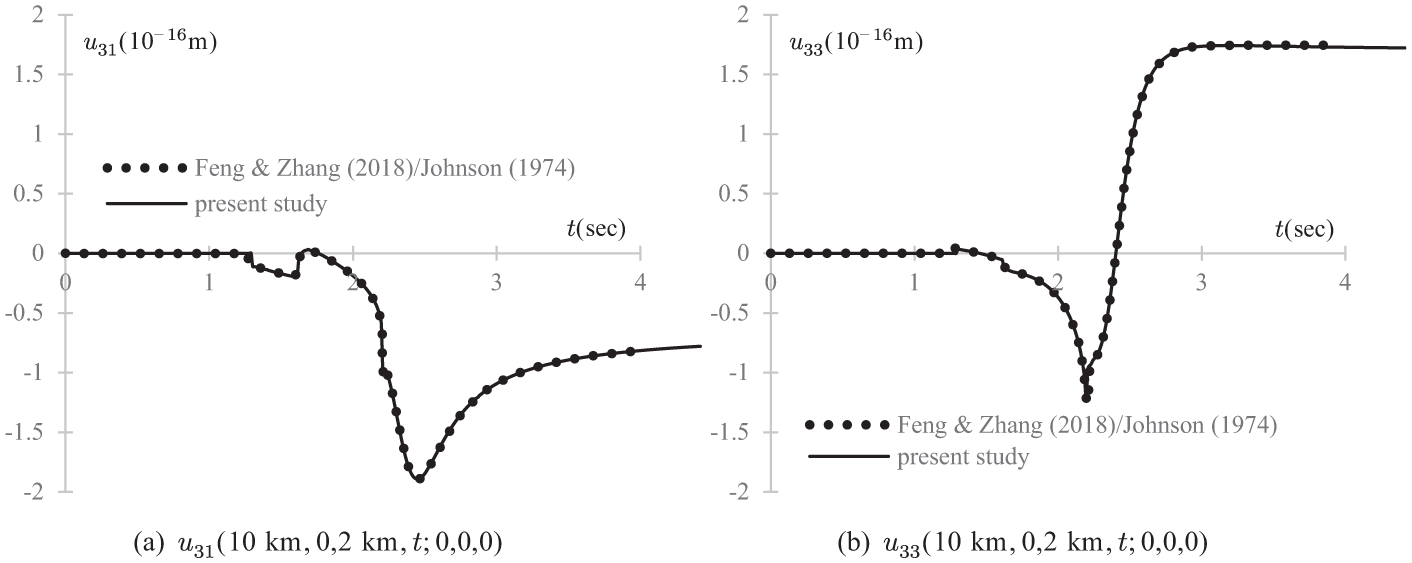
For the purpose of presenting numerical validation, examples of the results found in this paper and their comparison with the ones found in the previous investigations, the Green’s functions $u_{31}$ and $u_{33}$ given in equations (59) are evaluated and compared with the results found by Feng and Zhang [24]. Following that paper, the mechanical properties of the elastic half-space are assumed as $ρ = 3300 kg / m^{3}$ , $λ = μ = 7.04 \times 10^{10} N / m^{2}$ (hence Poisson’s ratio equals 0.25 in this case). Feng and Zhang [24] have considered boundary solutions for a point located on the surface and 10 km away from the epicentre, an interior source located at depth 2 km, but since we have treated interior solutions for a source located at the surface, the cases reciprocal to those used by Feng and Zhang [24] should be considered here. By reciprocity we have

\underset{the present paper}{\underset{︸}{u_{31} (10, 0, 2, t; 0, 0, 0)}} = \underset{Feng and Zhang (2018)}{\underset{︸}{u_{13} (10, 0, 0, t; 0, 0, 2)}}, \underset{the present paper}{\underset{︸}{u_{33} (10, 0, 2, t; 0, 0, 0)}} = \underset{Feng and Zhang (2018)}{\underset{︸}{u_{33} (10, 0, 0, t; 0, 0, 2)}}

(64)

in which the numbers 10 and 2 in equation (64) are in kilometres. Figure 7 shows the results of these comparisons, and as expected, a precise agreement is observed. Since the results of Feng and Zhang [24] have been themselves validated with Johnson’s classical results [21], our solutions are thus verified by Johnson’s paper as well.

Figure 7.

Comparison of the results of the present paper for the Green’s functions $u_{31}$ and $u_{33}$ with the ones reported by the previous studies. The mechanical properties of the half-space are $ρ = 3300 kg / m^{3}$ and $λ = μ = 70.4 GPa$ .

We now proceed to graphically represent the solution formulae in a dimensionless manner. Considering Figure 2, it is apparent that the terms having the factors $\cos φ_{0}$ and $\sin φ_{0}$ in the solutions (52) are respectively the contribution of the vertical and horizontal components of the point load p that is exerted onto the boundary. Accordingly, the solutions of equation (52) can be represented in the alternate form

\begin{matrix} u_{r} (r, θ, z, t) = u_{r (v)} (r, θ, z, t) + u_{r (h)} (r, θ, z, t), \\ u_{θ} (r, θ, z, t) = u_{θ (h)} (r, θ, z, t), \\ u_{z} (r, θ, z, t) = u_{z (v)} (r, θ, z, t) + u_{z (h)} (r, θ, z, t), \end{matrix}

(65)

where

\begin{matrix} u_{r (v)} (r, θ, z, t) = K (r, z, t), u_{r (h)} (r, θ, z, t) = \cos (θ - θ_{0}) [G (r, z, t) - H (r, z, t)], \\ u_{θ (h)} (r, θ, z, t) = \sin (θ - θ_{0}) [G (r, z, t) + H (r, z, t)], \\ u_{z (v)} (r, θ, z, t) = P (r, z, t), u_{z (h)} (r, θ, z, t) = \cos (θ - θ_{0}) Q (r, z, t) . \end{matrix}

(66)

As suggested by the notation, the functions having the symbols $(v)$ and $(h)$ in their indices denote the contribution of the vertical and horizontal components of the point load to the final solution, respectively; in this manner, $u_{r (v)}$ is the contribution of the vertical component of p to the solution $u_{r}$ , etc. It is noted that $u_{θ (v)}$ is identically zero since the vertical component of p produces axisymmetric solutions (no angular displacement).

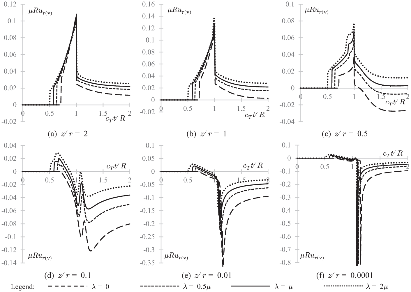
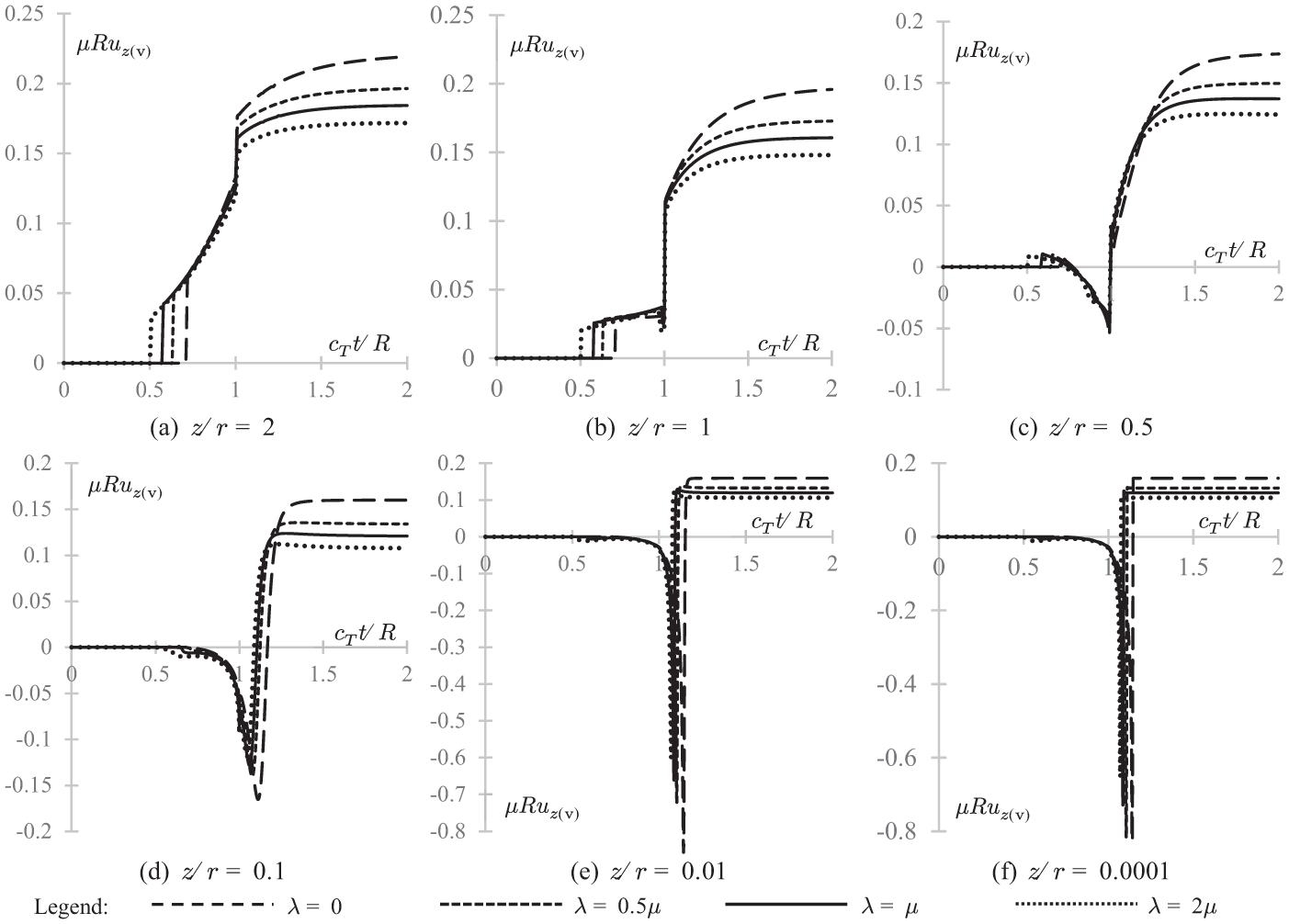
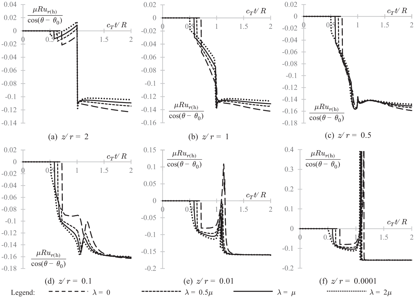
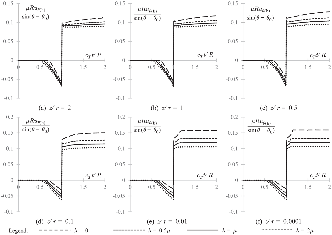
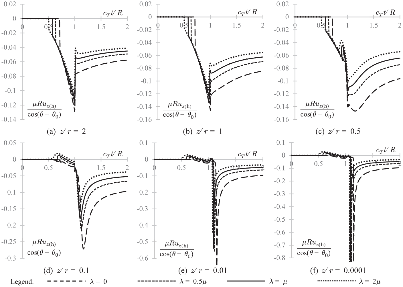
Dimensionless time-history diagrams are plotted for the five functions $u_{r (v)}, \dots, u_{z (h)}$ in Figure 8 to Figure 12 for six different $z / r$ ratios and for four different Lamé constant ratios. Evidently, the cases $λ = 0$ and $λ = μ$ correspond to Poisson’s ratio equal to 0 and 0.25, respectively; the latter case was used in [7, 9, 12, 19]. In these diagrams, the ordinate represents dimensionless displacement component, which is normalised by the magnitude of the point force (being unity here), while the abscissa represents the dimensionless time variable $τ = c_{T} t / R$ , where $R = \sqrt{r^{2} + z^{2}}$ is the spherical radius. Accordingly, the point $τ = 1$ always marks the arrival of the transverse wavefront (S-wave) that has travelled from the origin to the observation point in a straight path. This point is mentioned as a logarithmic singularity, whose effects are less apparent in shallow depths [10]. The arrival of the longitudinal wave (P-wave) occurs earlier at $τ = c_{T} / c_{L}$ when the time-history starts assuming non-zero values for the first time as one traces the graph from $τ = 0$ onwards.

Figure 8.

Dimensionless time-histories of the radial displacement due to the vertical component of the point load. The limiting values of the curves as $τ = c_{T} t / R$ tends to infinity are the classical elastostatic solutions.

Figure 9.

Dimensionless time-histories of the vertical displacement due to the vertical component of the point load. The limiting values of the curves as $τ = c_{T} t / R$ tends to infinity are the classical elastostatic solutions.

Figure 10.

Dimensionless time-histories of the radial displacement due to the horizontal component of the point load. The limiting values of the curves as $τ = c_{T} t / R$ tends to infinity are the classical elastostatic solutions.

Figure 11.

Dimensionless time-histories of the angular displacement due to the horizontal component of the point load. The limiting values of the curves as $τ = c_{T} t / R$ tends to infinity are the classical elastostatic solutions.

Figure 12.

Dimensionless time-histories of the vertical displacement due to the horizontal component of the point load. The limiting values of the curves as $τ = c_{T} t / R$ tends to infinity are the classical elastostatic solutions.

As observed in the time-history diagrams, apart from the P- and S-wavefronts, other tremors do form in the medium in certain zones. The most obvious of those, being the Rayleigh wavefront, arrives after P- and S-waves, and the effects of which become more projected at lower depths. As seen in parts (d), (e) and (f) in these figures, the Rayleigh wavefront is of mild amplitude in the zone $z / r = 0.1$ but quickly grows at $z / r = 0.01$ and forms a rather sharp spike at the even shallower depth ratio of $z / r = 0.0001$ . The only exception in this surface-effect phenomenon is the angular displacement $u_{θ}$ , in which Rayleigh waves do not contribute at all (see Figure 11); this is a vivid manifestation of the fact that Rayleigh waves are of P-SV origin rather than of SH origin. Because of the predominant influence that the Rayleigh wave has on the surface motions of an elastic solid, Lamb called it the main shock, while referring to effects of the P- and S-wavefronts as the minor tremor [4].

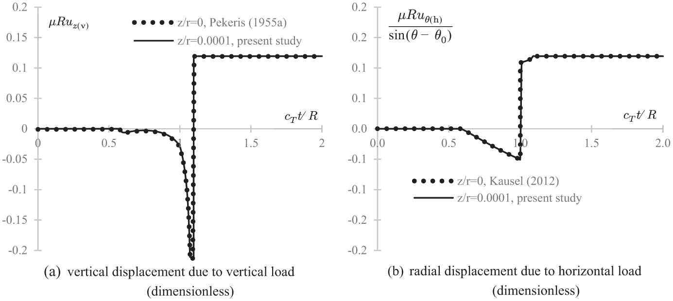
It can also be observed that for non-zero depths the amplitude of the Rayleigh wave is finite, while on the free surface, as Pekeris [7] and Chao [12] have shown, its amplitude becomes infinite. Nevertheless, the general shape of the time-history diagrams for vanishing $z / r$ are very much alike the corresponding diagrams for the surface solutions of Pekeris and Chao. In this regard for the case $λ = μ$ , Figures 8(f) and 9(f) are nearly identical to Pekeris’ diagrams [7] while Figures 10(f), 11(f) and 12(f) are almost indistinguishable from the diagrams found in Chao’s work [12]. In addition, our diagrams are in agreement with the ones given by Kausel [14] for $λ \neq μ$ . This shows that the solutions in the interior of the half-space can be evaluated for points in the immediate vicinity of the surface, to obtain nearly accurate time-history diagrams for the free surface ( $r > 0$ , $z = 0$ ). This is more clearly illustrated in Figure 13 in which two comparison examples are presented for the classical case $λ = μ$ . The same is true for epicentral solutions ( $r = 0$ , $z > 0$ ), although not shown in these diagrams; one may choose very large values of $z / r$ to have the representative curves for the solutions on the points situated directly under the point of application of the load.

Figure 13.

Comparisons between the boundary solutions [7,14] and interior solutions (evaluated in this paper) for points in the immediate vicinity of the boundary. The case $λ = μ$ is assumed here.

As mentioned earlier, Pekeris has also treated Lamb’s problem for a buried vertical point load, and derived solutions in the form of integrals for the surface points [9], which were later evaluated numerically [10]. Due to the elastodynamic reciprocal identity, the surface vertical and horizontal solutions of Pekeris are expected to be respectively identical to $u_{z (v)}$ and $u_{z (h)}$ in the interior, the latter divided by a factor of $\cos (θ - θ_{0})$ , in which the load is situated at the surface. This reciprocity is confirmed by comparing Figures 9 and 12 to the time-history diagrams given by Pekeris and Lifson [10].

Another curious, albeit less obvious, phenomenon observed here is the effect of indirect rays of wave at intermediate to shallow depths that arrive after the P-wave but before the direct S-wave. This can be seen more clearly in Figures 8(b) to (d), 9(b), 10(c) and 12(c). This wave is often referred to as the SP-wave, owing to the fact that it represents a ray that travels along a broken line trajectory, in part with the higher speed of P-waves, and in part with the lower speed of direct S-waves. The travel time of the SP-wave is shorter than that of direct S-wave, despite its longer trajectory [10]. In seismological terminology, the SP-waves are also termed head waves [19].

Lastly, the similarity of Figures 8(f) and 12(f) is also noteworthy. At the free surface, the radial displacement due to a vertical surface point load is essentially identical to the vertical displacement owing to a horizontal surface point load [with a factor of $\cos (θ - θ_{0})$ being omitted]. This fact was noticed by Chao [12] and is a consequence of reciprocity. We can readily verify this phenomenon analytically in our solutions: fixing $z = 0$ in (31) results in the two integrals $\tilde{K}$ and $\tilde{Q}$ becoming equal. Hence, due to equation (30), in the Laplace-domain, the vertical displacement due to a horizontal point load is $\cos (θ - θ_{0})$ times the radial displacement induced by a vertical point load; and the same is true in the time-domain, as one can takes the inverse Laplace transform from both sides of equation (30). It shall be emphasised, however, that this equality holds merely at the free surface, and as it can be observed lucidly in Figure 8(a) to (e) and Figure 12(a) to (e), the functions $u_{r (v)}$ and $u_{z (h)}$ behave quite differently at non-zero depths.

As mentioned earlier, one of the advantages of the solution formulae found in this paper is that they are valid for the complete permissible range of material constants. Therefore, these solution formulae can be used to investigate in detail the variations of displacements versus the elastic stiffness parameters. For that purpose, the solutions at a given interior point and at a given instant of time can be numerically calculated for different ratios of Lamé constants $λ / μ$ . Since $μ$ is non-negative and that the Poisson’s ratio is theoretically admissible in the interval $(- 1, \frac{1}{2})$ , the ratio $λ / μ$ can be assumed to be in the semi-infinite interval $(- \frac{2}{3}, \infty)$ . Here the functions $u_{z (v)}$ and $u_{z (h)}$ are considered at $τ = 1.5$ for demonstration examples in Figure 14. Hence, Figure 14(a) and (b) correspond to the time-history diagrams of Figures 9 and 12, respectively, at the point $τ = 1.5$ on the dimensionless time axis. An increase in the ratio $λ / μ$ , which is corresponding to an increase in Poisson’s ratio, can have different effects on the displacements. Here for example, as indicated in Figure 14, the function $u_{z (v)}$ is increased, while $u_{z (h)}$ is decreased as one increases the Poisson’s ratio of the material filled in the half-space under study; the points closest to the surface (curves $z / r = 0.0001$ in Figure 14) experience the most abrupt variations in both cases. Other functions defined by the equations (65) and (66) can be studied similarly. Accordingly, the solution formulae presented in this paper are not only useful for calculating time-history diagrams, but they can as well be utilised to study the effects of the Lamé constants ratio $λ / μ$ (or those of the Poisson’s ratio) on all elastodynamic displacement components at any interior point and at any instant of time.

Figure 14.

Examples of variations of solutions (at the particular instant $τ = 1.5$ ) versus the ratio of Lamé constants. The ratios $λ / μ = - 2 / 3$ and $λ / μ \to \infty$ correspond to Poisson’s ratio equal to $- 1$ and $1 / 2,$ respectively.

6. Conclusions

The transient motions in the interior of a homogeneous, isotropic, linear elastic half-space due to the impulsive excitation of a surface point load with arbitrary inclination and Heaviside time dependence have been rigorously investigated. Utilising the method of elastodynamic potentials and triple integral transforms, the corresponding non-axisymmetric initial boundary value problem has been treated. The inversion of the transformed solutions has been carried out analytically by defining the inversion procedure in the form of integral equations, the solutions of which have been obtained via a new modified version of Cagniard–Pekeris method. The exact interior solutions have been obtained as complicated non-elementary functions represented by integrals, which turn out to be finite despite their apparent complicated forms. The solutions have also been converted to the form of Green’s functions. The limit case of infinite time has been investigated analytically to obtain closed-form formulae for the limits of the solutions; the results of which are equivalent to the classical Boussinesq–Cerruti elastostatic solutions. The elastodynamic solutions have been then evaluated numerically for several points and various Lamé constants ratios to obtain time-history diagrams for the transient motions of the interior points. For points very close to the surface, the curves are found to be in agreement with the diagrams found in the literature. The solutions obtained here manifest vividly the formation of Rayleigh waves at shallow depths within the half-space. As expected, the amplitudes of such waves are finite inside the medium, but increase dramatically to infinity at the free surface.

Footnotes

Acknowledgements

The authors owe a great debt of gratitude to M.A. Dibaee for his valuable aid in the numerical evaluation of integrals occurring in this study.

Funding

The author(s) disclosed receipt of the following financial support for the research, authorship, and/or publication of this article: This work was supported in part by the University of Tehran (grant number 27840/1/09 awarded to Morteza Eskandari-Ghadi).

ORCID iD

Morteza Eskandari-Ghadi

References

Love

AEH.

A treatise on the mathematical theory of elasticity. New York: Dover Publications, 1944.

Achenbach

JD.

Wave propagation in elastic solids. Amsterdam: North-Holland, 1975.

Rayleigh

On waves propagated along the plane surface of an elastic solid. Proc Lond Math Soc 1885; 1: 4-11.

Lamb

On the propagation of tremors over the surface of an elastic solid. Philos Trans R Soc Lond 1904; 72: 128-130.

Graff

KF.

Wave motion in elastic solids. London: Oxford University Press, 1975.

Lapwood

ER.

The disturbance due to a line source in a semi-infinite elastic medium. Philos Trans R Soc Lond A 1949; 242: 63-100.

Pekeris

CL.

The seismic surface pulse. Proc Natl Acad Sci 1955; 41: 469-480.

Mooney

HM.

Some numerical solutions for Lamb’s problem. Bull Seismol Soci Am 1974; 64: 473-491.

Pekeris

CL.

The seismic buried pulse. Proc Natl Acad Sci 1955; 41: 629-639.

10.

Pekeris

Lifson

Motion of the surface of a uniform elastic half-space produced by a buried pulse. J Acoust Soc Am 1957; 29: 1233-1238.

11.

Cagniard

Réflexion et réfraction des ondes séismiques progressives. Paris: Gauthier-Villars, 1939.

12.

Chao

CC.

Dynamical response of an elastic half-space to tangential surface loadings. J Appl Mech 1960; 27: 559-567.

13.

Churchill

RV.

Operational mathematics. New York: McGraw-Hill, 1972.

14.

Kausel

Lamb’s problem at its simplest. Proc R Soc Lond A 2012; 469: 462-499.

15.

Richards

PG.

Elementary solutions to Lamb’s problem for a point source and their relevance to three-dimensional studies of spontaneous crack propagation. Bull Seismol Soc Am 1979; 69: 947-956.

16.

Eason

The displacements produced in an elastic half-space by a suddenly applied surface force. IMA J Appl Math 1966; 2: 299-326.

17.

Gakenheimer

Miklowitz

Transient excitation of an elastic half space by a point load traveling on the surface. J Appl Mech 1969; 36: 505-515.

18.

De Hoop

AT.

A modification of Cagniard’s method for solving seismic pulse problems. Appl Sci Res B 1960; 8: 349-356.

19.

Gakenheimer

DC.

Numerical results for Lamb’s point load problem. J Appl Mech 1970; 37: 522-524.

20.

Bakker

MCM

Verweij

Kooij

, et al. The traveling point load revisited. Wave Motion 1999; 29: 119-135.

21.

Johnson

LR.

Green’s function for Lamb’s problem. Geophys J R Astron Soc 1974; 37: 99-131.

22.

Pekeris

CL.

Solution of an integral equation occurring in impulsive wave propagation problems. Proc Natl Acad Sci 1956; 42: 439-443.

23.

Longman

IM.

Solution of an integral equation occurring in the study of certain wave-propagation problems in layered media. J Acoust Soc Am 1961; 33: 954-958.

24.

Feng

Zhang

Exact closed-form solutions for Lamb’s problem. Geophys J Int 2018; 214: 444-459.

25.

Eringen

Suhubi

ES.

Elastodynamics. New York: Academic Press, 1975.

26.

Sneddon

IN.

Fourier transforms. New York: McGraw-Hill, 1951.

27.

Sternberg

On the integration of the equations of motion in the classical theory of elasticity. Arch Rational Mech Anal 1960; 6: 34-50.

28.

Eskandari-Ghadi

A complete solution of the wave equations for transversely isotropic media. J Elast 2005; 81: 1–19.

29.

Eskandari-Ghadi

Pak

RYS

. Elastodynamics and elastostatics by a unified method of potentials for x3-convex domains. J Elast 2008; 92: 187–194.

30.

Apostol

TM.

Mathematical analysis. Reading, MA: Addison-Wesley, 1974.

31.

Watson

GN.

A treatise on the theory of Bessel functions. Cambridge: Cambridge University Press, 1922.

32.

Ahlfors

LV.

Complex analysis. New York: McGraw-Hill, 1966.

33.

Gaul

Kögl

Wagner

Boundary element methods for engineers and scientists: an introductory course with advanced topics. Berlin: Springer-Verlag, 2003.

Transient interior analytical solutions of Lamb’s problem

Abstract

Keywords

1. Introduction

2. Formulation of the initial boundary value problem

3. Potential functions and the method of solution

4. Analytical solution of the problem

4.1. General solution for the potential functions F and χ

4.2. Boundary conditions in the triply-transformed domain

4.3. Laplace-domain displacement components

4.4. General discussion on the Laplace transform inversion method

4.5. Inverse Laplace transforms of EIs of order ν = 0

4.6. Inverse Laplace transform of EIs of orders ν = 1 and 2

4.7. Time-domain displacement components

4.8. Time-domain displacement Green’s functions in Cartesian coordinate system

4.9. Solutions for infinite time: the classical Boussinesq–Cerruti solutions

5. Numerical evaluation of the solutions and graphical illustrations

6. Conclusions

Footnotes

Acknowledgements

Funding

ORCID iD

References

4.1. General solution for the potential functions F and $χ$

4.5. Inverse Laplace transforms of EIs of order $ν = 0$

4.6. Inverse Laplace transform of EIs of orders $ν = 1$ and 2