This paper aims to make some comparative studies between heterogeneous and homogeneous layers for nonlinear shear horizontal (SH) waves in terms of the heterogeneous and nonlinear effects. Therefore, with this aim, two layers are defined as follows: on the one hand, one layer consists of hyperelastic, isotropic, heterogeneous, and generalized neo-Hookean materials; on the other hand, another layer is made up of hyperelastic, isotropic, homogeneous, and generalized neo-Hookean materials. Moreover, it is assumed that upper boundaries are stress-free and lower boundaries are rigidly fixed. The method of multiple scales is used in both analyses, in addition to using the known solutions of the nonlinear Schrödinger (NLS) equation, called bright and dark solitary wave solutions; these comparisons are made, numerically, and then all results are given for the lowest branch of both dispersion relations, graphically. Moreover, these comparisons are observed both on a large scale and on a small scale, not only in terms of the bright and dark solitary wave solutions but also in terms of the heterogeneous and nonlinear effects.
Wave propagation in solids has two different behaviors. In one of them, the particles of the medium propagate in the direction of the wave propagation; these waves are known as longitudinal waves. Primary waves in seismology are an example of this type of wave motion. This behavior is also analogous to that of fluids. In the other, the particles of the medium propagate perpendicular to the direction of the wave propagation; these waves are known as transverse waves. Shear waves in seismology, also considered in this paper, are an example of this type of wave motion. In contrast, there is no analog to this behavior in fluids.
Elastic waves have been extensively studied by many investigators, because of their important applications in certain areas, such as signal processing in telecommunications, echography in medicine, nondestructive testing in metallurgy, and earthquakes in seismology, to name a few. As seen in the mentioned applications, to study with elastic waves is worthy of applied sciences. Some scientifically valuable discussions on these waves in solids, including the fundamental theorems of elastodynamics, the linearized theory of elasticity, various mathematical methods of solutions, some applications of these waves, various types of waves and waveguides, and so on, can be found in [1–5] and references therein, in addition studies of nonlinear waves, evaluation equations, perturbation methods, solitary wave solutions, and so on, can be found in [6–14].
It is known that elastic waves in linear media can be described by linear differential equations in which the superposition principle applies. However, these waves in nonlinear media can be modeled by nonlinear differential equations in which the superposition principle does not generally apply. In other words, nonlinear wave equations are more difficult to analyze mathematically than linear wave equations, owing to the lack of the general theory of nonlinear equations. Therefore, many investigations of nonlinear wave propagation treat waves individually. Overcoming the difficulty of nonlinearity, asymptotic perturbation methods are generally used. Striking a balance between dispersion and nonlinearity in the analysis, various types of nonlinear evaluation equation, such as Korteweg–de Vries (K–dV), nonlinear Schrödinger (NLS), and Boussinesq (BE), are found for the nonlinear modulation of the wave propagation. In this direction, some problems are studied in [15–27] and relevant studies therein. Moreover, not to leave them unmentioned, shear waves (or surface shear waves) in linear or nonlinear media are also found in [28–32], including exact solutions of shear waves, layered structures, heterogeneity, and so on. Furthermore [33], is a good reference for heterogeneous materials.
Linear shear horizontal (SH) wave (or surface SH wave) solutions in homogeneous media are well known [2, 5]. Nonlinear SH wave (or surface SH wave) solutions in homogeneous media are also known in different waveguides, such as in a layer [17], a plate [16], a two-layered plate [15], or a layered half-space [27]. However, nonlinear SH wave (or surface SH wave) solutions in heterogeneous media are not well known, owing to the difficulty of nonlinearity and heterogeneity. This difficulty can be seen in [28], even though linear SH wave solutions in heterogeneous media are considered there, and then exact solutions are given only in terms of a few simple types of heterogeneity, in addition to looking at large coefficients of differential equations in [18, 19] and references in [20]. The propagation of nonlinear SH waves in a heterogeneous layer is considered in [18, 19], assuming that the layer consists of hyperelastic, isotropic, and generalized neo-Hookean materials. In this paper, using this problem, the propagation of nonlinear SH waves in a heterogeneous layer will be reconsidered in some comparative studies between heterogeneous and homogeneous materials in terms of heterogeneous and nonlinear effects. To consider SH waves in a connection between heterogeneous and homogeneous materials may be interesting for understanding the complex mechanical behavior of the Earth, because it is known that the crust and the mantle, called the layers of the Earth, contain heterogeneous materials, in addition to other important applications of heterogeneous materials. In the next section, two problems will be defined precisely for some comparative studies.
2. Problems and materials
The spatial and material coordinates of a point referred to the same rectangular Cartesian system of axes are and , respectively. A layer with finite thickness overlying a rigid substratum is taken into account. The layer is considered between the planes and overlying a semi-infinite substratum in the region . In addition, it is assumed that the boundary is free of traction and the boundary is rigidly fixed. An SH wave supposed to propagate along the X-axis can be defined by
where indicates the displacement in the Z direction of a particle and t indicates the time. For some comparative studies, two problems will be defined by using this layer, and this mentioned wave.
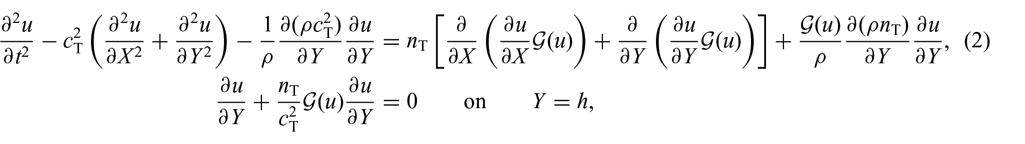
On the one hand, in the heterogeneous problem, the propagation of SH waves in this layer is considered with different material properties, such as hyperelastic, isotropic, heterogeneous, and generalized neo-Hookean. Therefore, considering small but finite amplitude wave motion, the governing equation and boundary conditions can be written as follows:
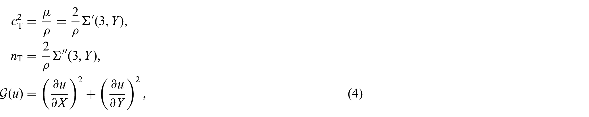
Here, the linear shear wave velocity and the nonlinear material function are denoted by and , respectively, in addition to the following definitions for , , and :
where indicates the strain energy function of the layer. In this article, for the heterogeneous problem, is a continuously differentiable function of Y, and the following suitable choices on the functions and ,
are used, where and are constants, and is a parameter to observe the heterogeneous effect. Using equation (5), is obtained. Moreover, for a numerical study, the function is chosen as
where is a constant and is a parameter to observe the nonlinear effect (for more information on this problem, see [18, 19]).
As seen in equation (5), and are continuously differentiable functions of Y in particular not in general, i.e, and in the mathematical sense, assuming that and contain the initial constants and the parameters of a medium in the physical sense. That is why the choice of equation (5) is suitable for evading the difficulty of nonlinearity since science suffers from the lack of the general theory of nonlinear partial differential equations (PDEs) that is seen in the known mathematics. Otherwise, this analysis will be hard to study with the known theory of nonlinear PDEs. At this point, the author thinks that solving difficult equations in science needs good theories.
On the other hand, in the homogeneous problem, the propagation of SH waves in the geometrically same layer is considered for material properties such as hyperelastic, isotropic, homogeneous, and generalized neo-Hookean (for a similar problem, see [17]). Because of the material choices, , , , and are constants in this case. In this paper, some comparative studies between homogeneous and heterogeneous problems will be considered, and so, without loss of meaning, the constants , , , and for the homogeneous problem are also used. Therefore, equations (2) and (3) are also valid for the homogeneous problem, meaning that the limits of the functions in equations (5) and (6) as and yield the coefficient functions of the governing equation and the boundary conditions of the homogeneous problem. Furthermore, the constituent material of the layer softens in shear if (or, equivalently, since the term is always positive) and hardens in shear if (or, equivalently, since the term is always positive). In addition, equation (2) is reducible to the equation of the linear SH waves in a homogeneous (or heterogeneous) medium by using the condition (or ) [3].
3. Analysis and method
In this section, short review analyses of both problems, defined as heterogeneous and homogeneous problems in the previous section, will be given. As seen in the definitions of heterogeneous and homogeneous problems, the heterogeneous problem is more general than the homogeneous one. Therefore, the first focus will be on the analysis of the heterogeneous problem. Using the method of multiple scales given in [8], the heterogeneous problem is extensively analyzed in [18, 19]. In this analysis, keeping a balance between dispersion and nonlinearity, it is shown that the self-modulation of nonlinear SH waves can be described by the NLS equation, and then, considering the known solitary wave solutions of the NLS equation, the bright and dark solitary SH wave solutions are found, respectively. Therefore, for a short review, there are two crucial equations to remember from the mentioned asymptotic analysis of the heterogeneous problem. One of them is called the dispersion relation, given by
where the nondimensional parameter observes the heterogeneous effect, the constant n denotes a branch of the dispersion relation , and . Moreover, nondimensional functions of the nondimensional wavenumber , such as the phase velocity, group velocity, and angular frequency, are designated as , , and , where dimensional functions of the dimensional wavenumber k, such as the phase velocity, shear wave velocity, group velocity, and angular frequency, are denoted by , and w, respectively. The other is called the NLS equation, written as
where denotes the nondimensional amplitude of the wave motion. To make the discussion clear at this point, the variables can be given as follows: and , where parameters of asymptotic analysis with a small positive are given as . Moreover, the coefficient carries the dispersion depending on the linear constants and the heterogeneous parameter A, whereas the coefficient also carries the nonlinearity depending on the nonlinear constant and the nonlinear parameter , where . Furthermore, in the given numerical analysis of the heterogeneous problem, owing to the heterogeneous parameter A and the nonlinear parameter , not only the heterogeneous effect but also the nonlinear effect is well observed for the bright and dark solitary SH waves, respectively. In the given analysis, there is no restriction on the heterogeneous and nonlinear parameters. Therefore, the limit of the given analysis of the heterogeneous problem as and (or as and ) exactly corresponds to the analysis of the homogeneous problem. Note that, because of using different material choices in both problems, it is clear that the dispersion relation and the NLS equation for each problem are different from each other. Performing a numerical analysis for both problems, based on the mentioned asymptotic analyses, this difference will be given as some comparative studies between homogeneous and heterogeneous materials in the next section. For more information on the antiplane motion, the analysis, and so on, the reader is referred to [18, 19].
4. Comparisons and conclusion
Using the NLS equation, known as a famous evaluation equation in wave propagation, some comparisons between heterogeneous and homogeneous problems for nonlinear SH waves in terms of heterogeneous and nonlinear effects will be given here. It is known that the sign of behaves as a criterion for the existence of solutions of the NLS equation. The existence of the traveling wave solutions of the NLS equation of the form
is based on the sign of , where and , and are constants. One example of these types of solution to the NLS equation, called the bright solitary wave solution, will be considered as follows:
Bright solitary wave solution. Considering the condition , one of the well known solutions of the NLS equation, called a bright solitary wave solution, will be given here. For , if and as , then one finds
where and . When , there are no solutions of the NLS equation corresponding to equation (10) for the case . However, a solution of the following form exists for [6, 7, 34, 35].
Dark solitary wave solution. Considering the condition , one of the well known solutions of the NLS equation, called a dark solitary wave solution, will be considered here. Let us focus on the form of the solution to the NLS equation, as
For , if and as , then the solutions and F are found to be [6, 7, 34, 36].
where is a constant and and are given as
As recalled in these short review analyses, the sign of depends on the sign of since the term is always positive, where is a real number. Therefore, there are three possible cases for the constant as follows.
Case 1. If , the linear SH wave equation is obtained; but it is not interesting to consider since it has the same form solution as the first-order problem of the asymptotic analysis given in [18, 19] with a small difference between amplitudes (see also [30]).
Case 2. If , then for all in both analyses. Therefore, using the short review given in equations (11) to (13), the existence of the nonlinear dark solitary SH wave solution in a heterogeneous layer can be found in [19]. In addition, using the limit in this analysis, the existence of the nonlinear dark solitary SH wave solution in a homogeneous layer can be deduced from there. In this case, three possible comparisons come up:
Comparison 1. A comparison between heterogeneous and homogeneous layers for the nonlinear dark solitary SH waves in terms of the nonlinear effect can be seen in this part, or equivalently, this mentioned comparison in sense of mathematics can be expressed as
where
Comparison 2. A comparison between heterogeneous and homogeneous layers for the nonlinear dark solitary SH waves in terms of the heterogeneous effect can be given in this part, or equivalently, this mentioned comparison in sense of mathematics can be expressed as
where
Comparison 3. A comparison between heterogeneous and homogeneous layers for the nonlinear dark solitary SH waves in terms of the mixed effect (the both heterogeneous and nonlinear effects) can be given in this part, or equivalently, this mentioned comparison in sense of mathematics can be expressed as
where and
Case 3. If , then for all in both analyses. Therefore, using the short review given in equation (10), the existence of the nonlinear bright solitary SH wave solution in a heterogeneous layer can be found in [18]. In addition, using the limit in this analysis, the existence of the nonlinear bright solitary SH wave solution in a homogeneous layer can be deduced from there. In this case, three possible comparisons come up:
Comparison 4. A comparison between heterogeneous and homogeneous layers for the nonlinear bright solitary SH waves in terms of the nonlinear effect can be seen in this part, or equivalently, this mentioned comparison in sense of mathematics can be expressed as
where
Comparison 5. A comparison between heterogeneous and homogeneous layers for the nonlinear bright solitary SH waves in terms of the heterogeneous effect can be seen in this part, or equivalently, this mentioned comparison in sense of mathematics can be expressed as
Comparison 6. A comparison between heterogeneous and homogeneous layers for the nonlinear bright solitary SH waves in terms of the mixed effect can be given in this part, or equivalently, this mentioned comparison in sense of mathematics can be expressed as
where and
In what follows, five of these six comparisons are made; the focus will firstly be on the first comparison, and secondly continue with the second one, and so on. For making all comparisons, a fixed common branch of both dispersion relations is needed; the lowest branch, i.e., , is chosen, in addition to fixing linear constants and , i.e., . Moreover, in this numerical calculation, the nonlinear constants for softening and hardening models are chosen as (for the bright soliton) and (for the dark soliton), respectively. Note that the following results are independent of the choices (linear model) and (nonlinear models), because of the nondimensional analysis. These are only to show the signs of the models.
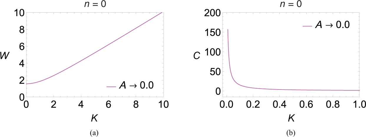
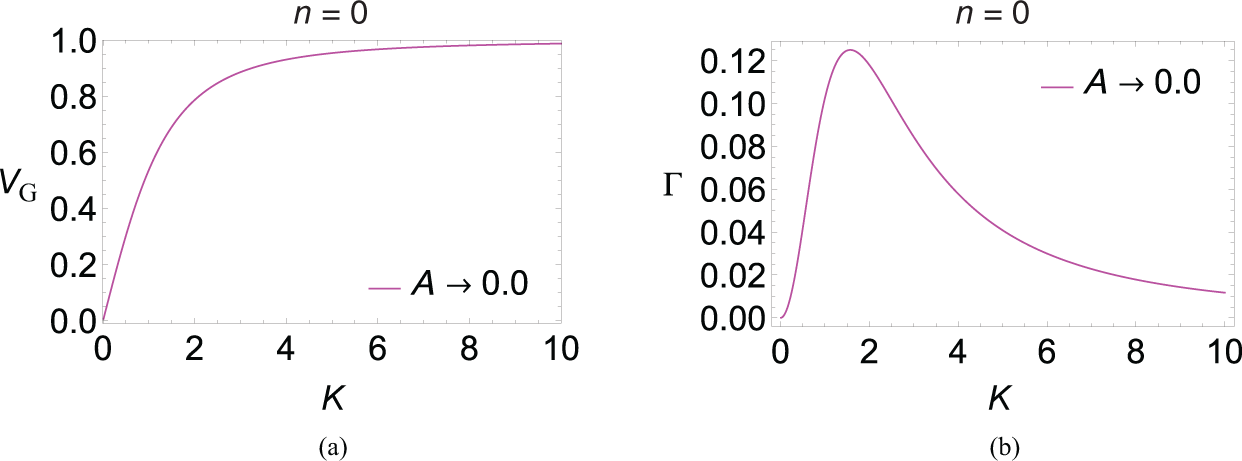
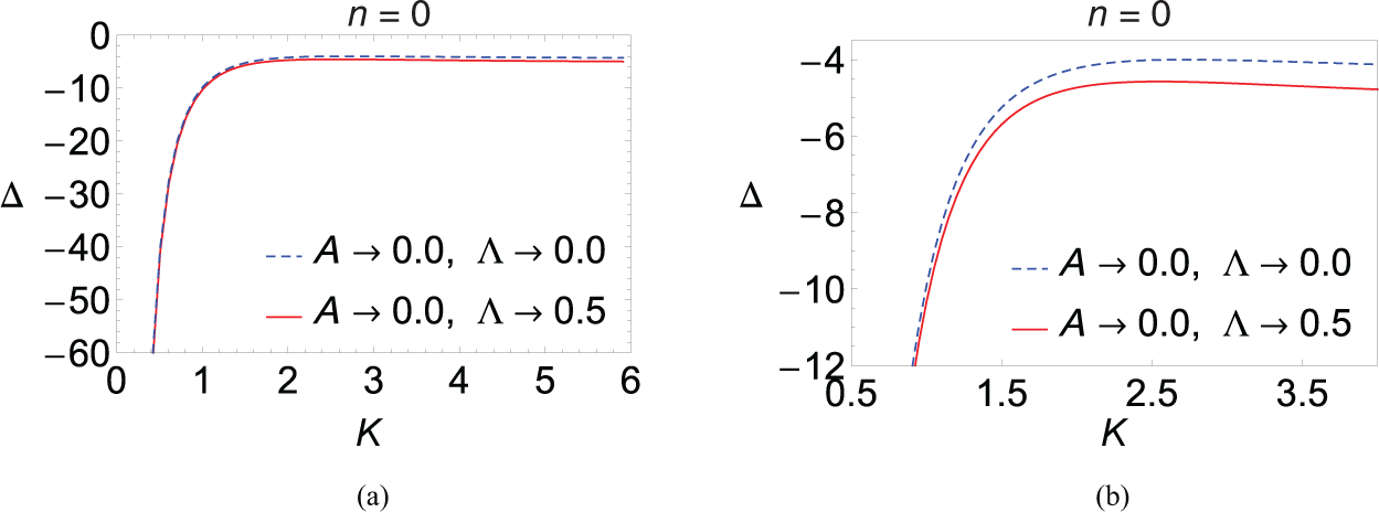
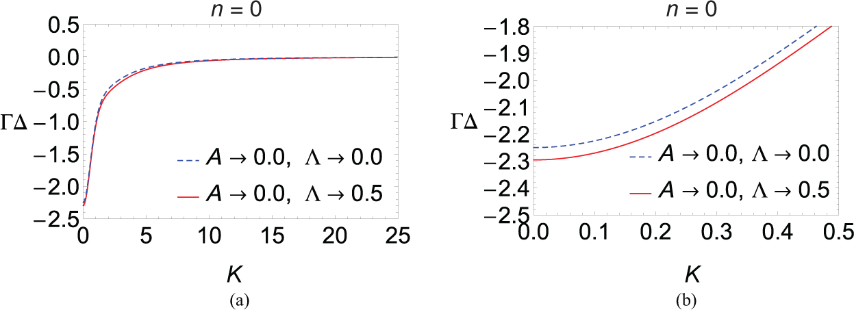
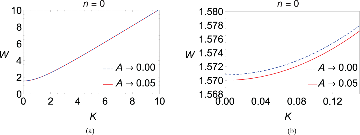
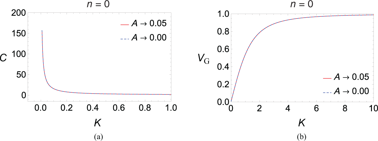
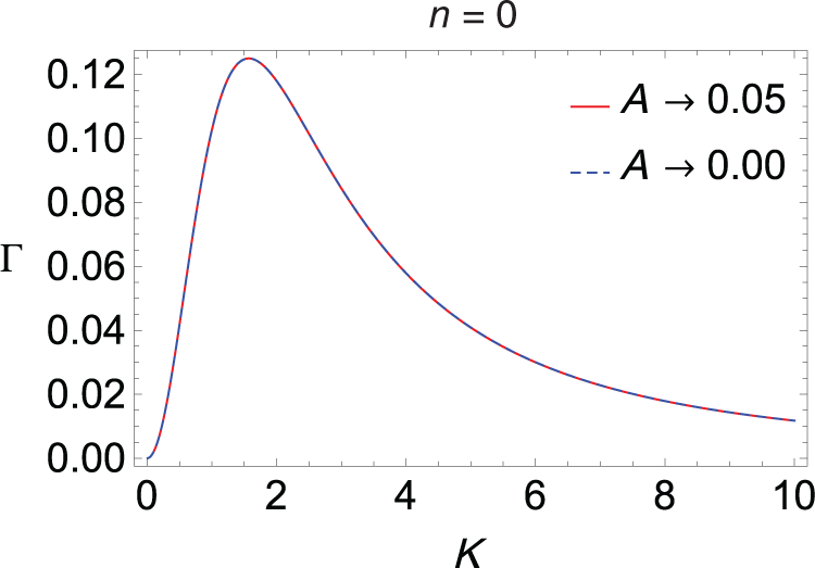
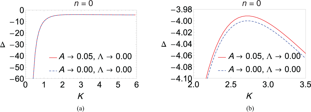
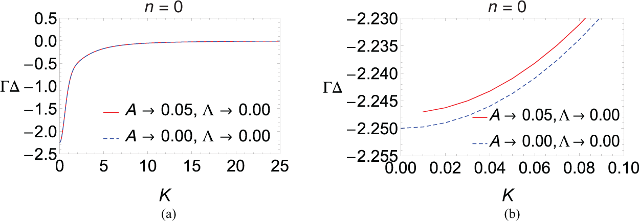
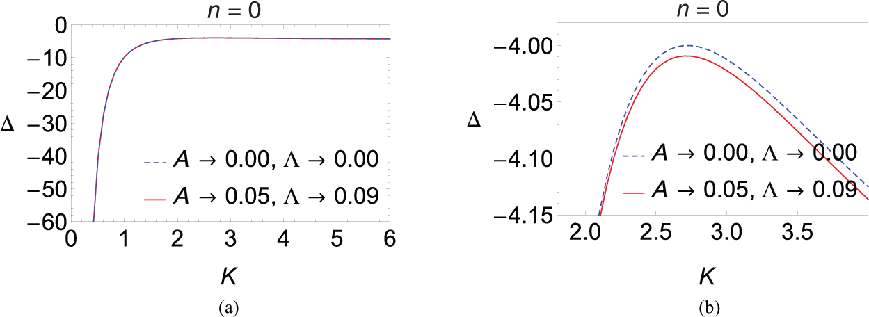
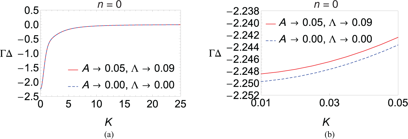
Let us start with the first comparison. In the asymptotic analysis of the heterogeneous problem, two material effects, called heterogeneous and nonlinear effects, are observed. For this mentioned comparative study, the heterogeneous effect must be fixed in both analyses; thus . Considering the mentioned linear model, the variations of and versus K (the common part of both analyses) are presented in Figures 1 and 2, respectively. Moreover, considering the mentioned linear and nonlinear models, continuing with the fixed heterogeneous effect and changing the nonlinear effect from to , the nonlinear effect on the coefficient and , as a comparative study between heterogeneous and homogeneous layers for nonlinear dark solitary SH waves, is then observed on large and small scales in Figures 3 and 4, respectively. To complete this comparison, to consider the following hardening material model
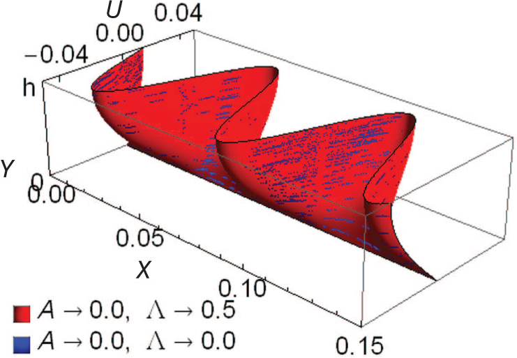
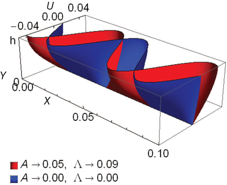
the first comparison is also made for the deformation fields of the planes of the layers, and is plotted in Figure 5.
(a) Variation of W with respect to K with . (b) Variation of C with respect to K with .
(a) Variation of with respect to K with . (b) Variation of with respect to K with .
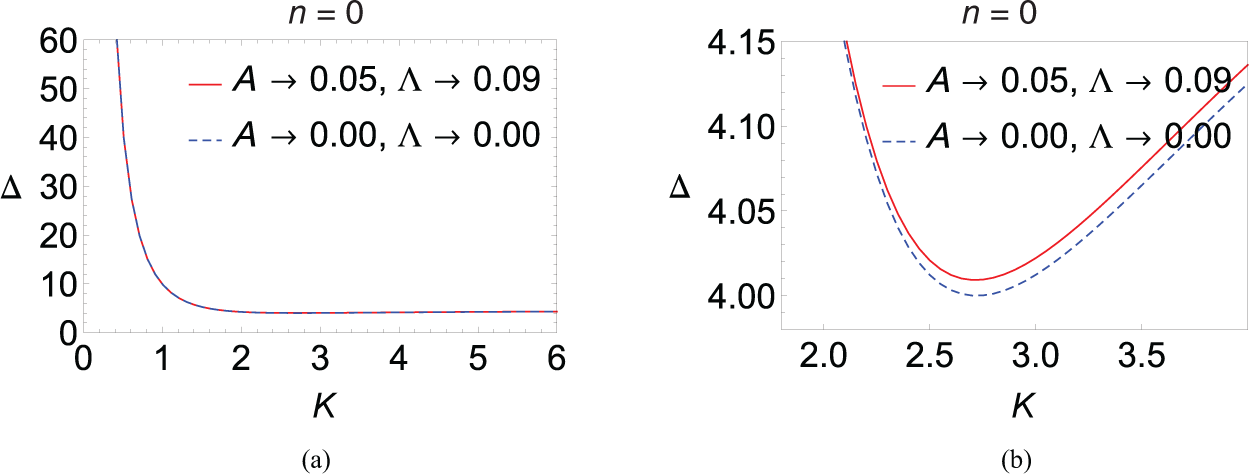
(a) Variation of with respect to K, with , and , on a large scale. (b) Variation of with respect to K, with , and , on a small scale.
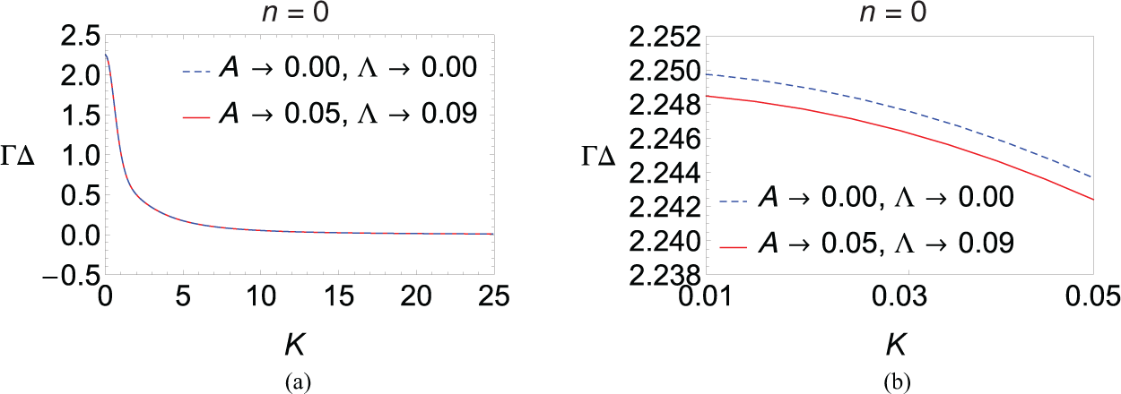
(a) Variation of with respect to K, with , and , on a large scale. (b) Variation of with respect to K with , and , on a small scale.
Deformation fields of the planes of the layers with , and , .
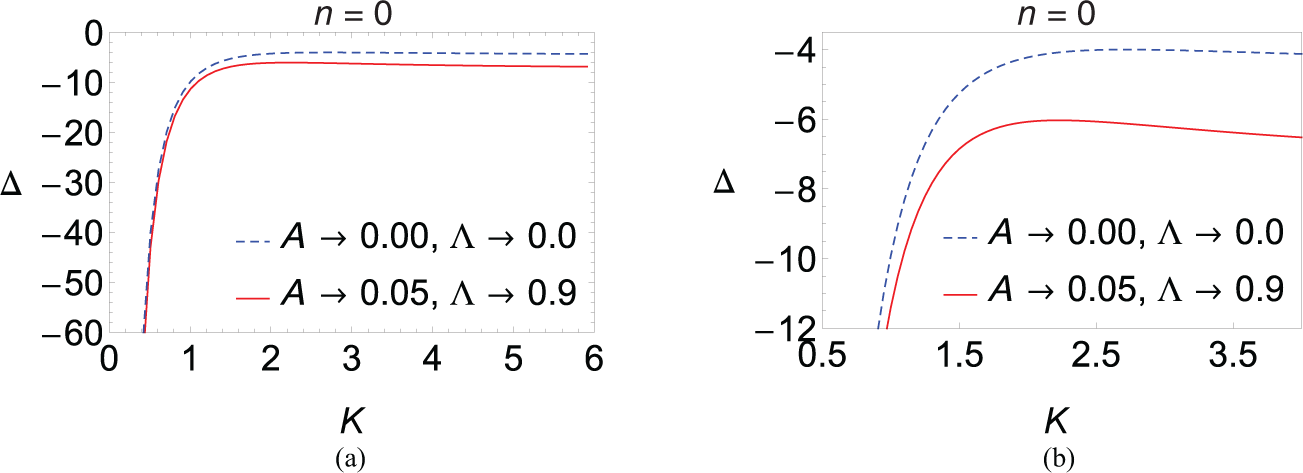
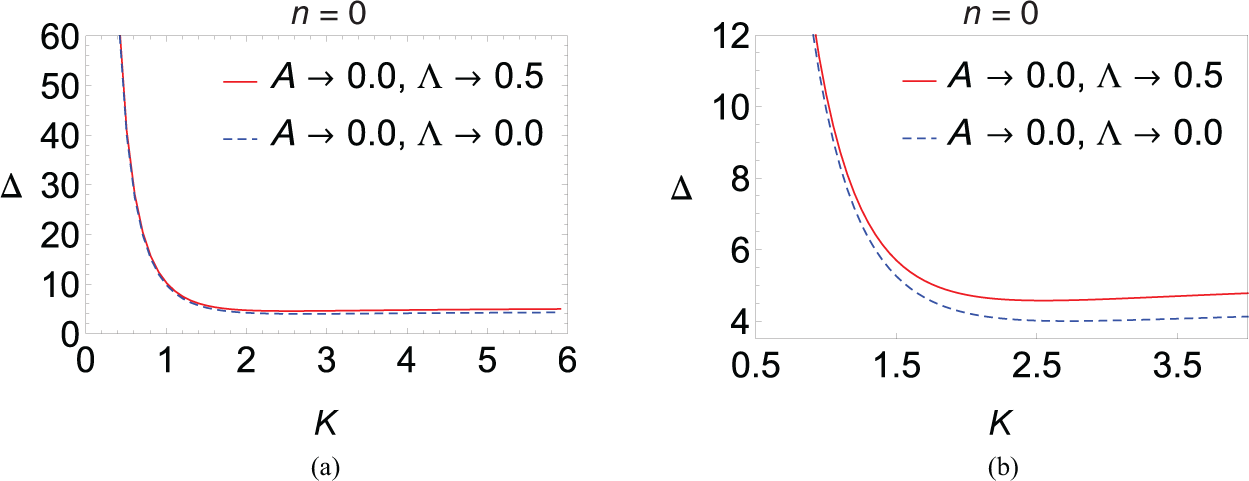
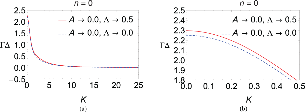
Let us now continue with the second comparison. Considering the mentioned linear model and changing the heterogeneous effect from to , the respective variations of W as a function of K on large and small scales are plotted in Figure 6, the respective variations of C and as a function of K are plotted in Figure 7, and the variation of as a function of K is plotted in Figure 8. For this comparative study, it is necessary to fix the nonlinear effect in both analyses, thus . Considering the mentioned linear and nonlinear models and changing the heterogeneous effect from to , the heterogeneous effect on the coefficients and as a comparative study between heterogeneous and homogeneous layers for nonlinear dark solitary SH waves is shown on large and small scales in Figures 9 and 10, respectively. To complete this part, again, to consider the hardening material model (equation (14)), this comparison is also made for the deformation fields of the planes of the layers, and is plotted in Figure 11.
(a) Variation of W with respect to K with and on a large scale. (b) Variation of W with respect to K with and on a small scale.
(a) Variation of C with respect to K with and . (b) Variation of with respect to K with and .
Variation of with respect to K with and .
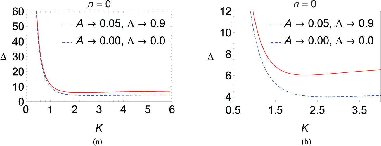
(a) Variation of with respect to K with , and , on a large scale. (b) Variation of with respect to K with , and , on a small scale.
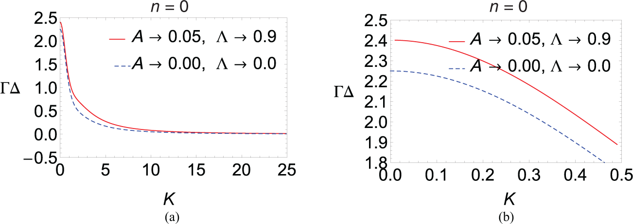
(a) Variation of with respect to K with , and , on a large scale. (b) Variation of with respect to K with , and , on a small scale.
Deformation fields of the planes of the layers with , and , .
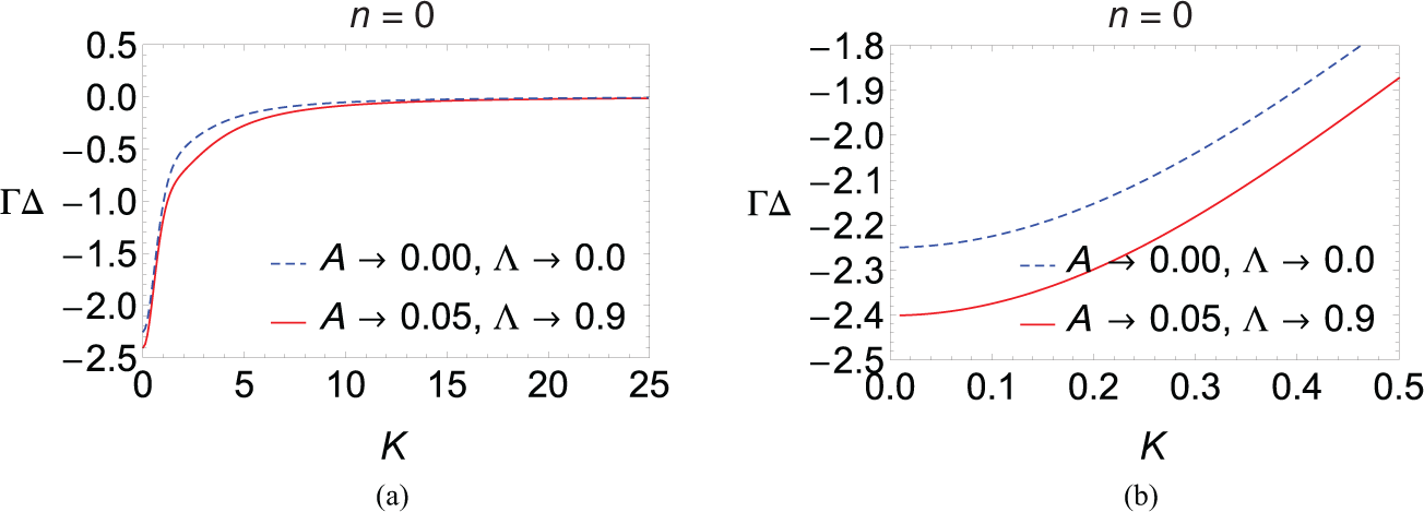
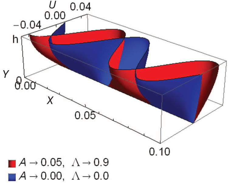
For the third comparison, the numerical analysis will be deep since the analysis of the heterogeneous problem is strong in this case. In this part, the mixed effect (both heterogeneous and nonlinear effects) is considered using the limits and or and as models for the heterogeneous problem, in addition to continuing with the homogeneous problem. For this comparison, Figures 6 to 8 are again needed. Moreover, considering the first heterogeneous model, the mixed effect on the coefficients and , as a comparative study between heterogeneous and homogeneous layers for nonlinear dark solitary SH waves, is shown on large and small scales in Figures 12 and 13, respectively. To complete this part, to consider the hardening material model (equation (14)), this comparison is also made for the deformation fields of the planes of the layers, and is plotted in Figure 14. Similarly, using Figures 6 to 8 and considering the second heterogeneous model, the mixed effect on the coefficients and as a comparative study between heterogeneous and homogeneous layers for nonlinear dark solitary SH waves is shown on large and small scales in Figures 15 and 16, respectively. To complete this part, to consider the hardening material model (equation (14)), this comparison is also made for the deformation fields of the planes of the layers, and is plotted in Figure 17.
(a) Variation of with respect to K with , and , on a large scale. (b) Variation of with respect to K with , and , on a small scale.
(a) Variation of with respect to K with , and , on a large scale. (b) Variation of with respect K with , and , on a small scale.
Deformation fields of the planes of the layers with , and , .
(a) Variation of with respect to K with , and , on a large scale. (b) Variation of with respect to K with , and , on a small scale.
(a) Variation of with respect to K with , and , on a large scale. (b) Variation of with respect to K with , and , on a small scale.
Deformation fields of the planes of the layers with , and , .
For the fourth comparison, again using Figures 1 and 2, for the fixed heterogeneous effect and changing the nonlinear effect from to , the nonlinear effect on the coefficient and , as a comparative study between heterogeneous and homogeneous layers for nonlinear bright solitary SH waves, is shown on large and small scales in Figures 18 and 19, respectively. To complete this comparison, to consider the softening material model
this comparison is also made for the deformation fields of the planes of the layers, and is plotted in Figure 20.
(a) Variation of with respect to K with , and , on a large scale. (b) Variation of with respect to K with , and , on a small scale.
(a) Variation of with respect to K with , and , on a large scale. (b) Variation of with respect to K with , and , on a small scale.
Deformation fields of the planes of the layers with , and , .
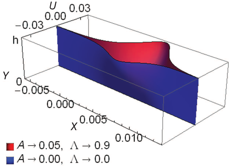
For the last comparison, again, the numerical analysis will again be deep. The mixed effect is considered using the limits and or and , as mentioned before, in addition to continuing with the homogeneous model. For this comparison, Figures 6 to 8 are again needed. Moreover, considering the first heterogeneous model, the mixed effect on the coefficients and , as a comparative study between heterogeneous and homogeneous layers for nonlinear bright solitary SH waves, is shown on large and small scales in Figures 21 and Figure 22, respectively. To complete this part, to consider the softening material model (equation (15)), this comparison is also made for the deformation fields of the planes of the layers, and is plotted in Figure 23. Similarly, using Figures 6 to 8 and considering the second heterogeneous model, the mixed effect on the coefficients and , as a comparative study between heterogeneous and homogeneous layers for nonlinear bright solitary SH waves, is shown on large and small scales in Figures 24 and 25, respectively. To complete this part, to consider the hardening material model (equation (15)), this comparison is also made for the deformation fields of the planes of the layers, and is plotted in Figure 26.
(a) Variation of with respect to K with , and , on a large scale. (b) Variation of with respect to K with , and , on a small scale.
(a) Variation of with respect to K with , and , on a large scale. (b) Variation of with respect to K with , and , on a small scale.
Deformation fields of the planes of the layers with , and , .
(a) Variation of with respect to K with , and , on a large scale. (b) Variation of with respect to K with , and , on a small scale.
(a) Variation of with respect to K with , and , on a large scale. (b) Variation of with respect to K with , and , on a small scale.
Deformation fields of the planes of the layers with , and , .
In such an analysis, it can be emphasized that the dispersion and the nonlinearity can be carried by and , respectively. As seen in Figure 2(b), approaches zero as K approaches zero, at where has a minimum. In other words, the dispersion vanishes at . Also, from Figure 3(a) and Figure 18(a), it is seen that approaches as K approaches zero. Equivalently, decays or grows unboundedly at . At such a critical point, i.e., , it is not possible to balance the nonlinearity and the dispersion with the given analysis. Therefore, the analyses of heterogeneous and homogeneous problems do not work well for such a case. Perhaps some researchers may try to improve the analysis at this point in a future study. Furthermore, for the stability of solutions of such problems and other types of solutions of the NLS equation, the reader is referred to [27]. Also, further comparative studies for elastic waves can be found in [37, 38]; for the problem of how to maintain the motion in such layers without body forces, the reader is referred to [27, 39]. Finally, however, although a layer structure is considered here, the problem given in [20] and references therein is useful for a plate structure too, as will be seen elsewhere.
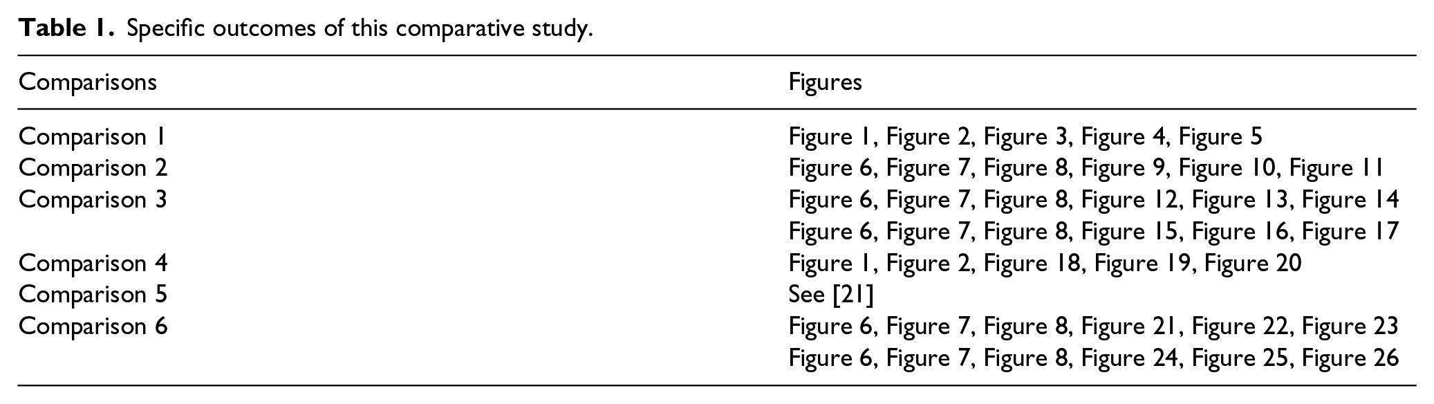
In this study, it is seen that, mathematically, the heterogeneous problem is more general than the homogeneous one. In other words, a generalization of homogeneous materials is seen here. This generalization allows us to make a hierarchy between materials not only for heterogeneous and homogeneous materials but also for submaterials (new types) of heterogeneous materials. During this study, heterogeneous, nonlinear, and mixed effects are well observed both on large and small scales. Maybe, they are useful effects for applied sciences, such as engineering, material science, and so on. Moreover, the amplitude of dark solitary SH waves is not affected too much by these mentioned effects; whereas, the amplitude of bright solitary SH waves is greatly affected. It is seen that there are many graphics to follow. Therefore, the summary in Table 1 may be useful.
We thank the editor for the enormous and polite review process and the referee for the great constructive comments that led to the improvements in this paper.
Funding
The author(s) received no financial support for the research, authorship, and/or publication of this article.
ORCID iD
Dilek Demirkuş
References
1.
AchenbachJD.Wave propagation in elastic solids. Amsterdam: North-Holland, 1973.
2.
EringenACSuhubiES.Elastodynamics, vol. 2. New York: Academic Press, 1975.
3.
EwingWMJardetskyWSPressF.Elastic waves in layered media. New York: McGraw-Hill, 1957.
4.
FarnellGW. Types and properties of surface waves. In: OlinerAA (ed.) Acoustic surface waves. Berlin: Springer, 1978, 13–60.
5.
GraffKF.Wave motion in elastic solids. New York: Dover, 1975.
6.
AblowitzMJClarksonPA.Solitons, nonlinear evolution equations and inverse scattering. Cambridge: Cambridge University Press, 1991.
7.
DoddRKMorrisHCEilbeckJC, et al. Solitons and nonlinear wave equations. London: Academic Press, 1982.
8.
JeffreyAKawaharaT.Asymptotic methods in nonlinear wave theory. Boston: Pitman, 1981.
9.
MauginGA. Physical and mathematical models of nonlinear waves in solids. In: JeffreyAEngelbrechtJ (eds.) Nonlinear waves in solids. New York: Springer, 1994, 109–233.
10.
NorrisA. Finite amplitude waves in solids. In: HamiltonMFBlackstockDT (eds.) Nonlinear acoustics. San Diego: Academic Press, 1998, 263–277.
11.
ParkerDF. Nonlinear surface acoustic waves and waves on stratified media. In: JeffreyAEngelbrechtJ (eds.) Nonlinear waves in solids. New York: Springer, 1994, 289–347.
12.
PorubovAV.Amplification of nonlinear strain waves in solids. Singapore: World Scientific, 2003.
13.
SamsonovAM. Nonlinear strain waves in elastic waveguides. In: JeffreyAEngelbrechtJ (eds.) Nonlinear waves in solids. New York: Springer, 1994, 349–382.
14.
WhithamGB.Linear and nonlinear waves. New York: John Wiley and Sons, 1974.
15.
AhmetolanSTeymurM.Nonlinear modulation of SH waves in a two-layered plate and formation of surface SH waves. Int J Non Linear Mech2003; 38: 1237–1250.
16.
AhmetolanSTeymurM.Nonlinear modulation of SH waves in an incompressible hyperelastic plate. Z Angew Math Phy2007; 58: 457–474.
17.
DemirkuşDTeymurM. Shear horizontal waves in a nonlinear elastic layer overlying a rigid substratum. Hacet J Math Stat2017; 46(5): 801–815.
18.
DemirkuşD. Nonlinear bright solitary SH waves in a hyperbolically heterogeneous layer. Int J Non Linear Mech2018; 102: 53–61.
19.
DemirkuşD.Nonlinear dark solitary SH waves in a heterogeneous layer. TWMS J Appl Eng Math2019. DOI: 10.26837/jaem.627563.
20.
DemirkuşD.Antisymmetric dark solitary SH waves in a nonlinear heterogeneous plate. Z Angew Math Phys2019; 70(6): 173.
21.
DemirkuşD. A comparison between heterogeneous and homogeneous layers for bright solitary shear horizontal waves in terms of heterogeneous effect. In: AltenbachHEremeyevVAPavlovI, et al. (eds.) Nonlinear wave dynamics of materials and structures (Advanced Structured Materials, vol. 122). Cham: Springer, 2020.
22.
DestradeMGorielyMASaccomandiG.Scalar evolution equations for shear waves in incompressible solids: a simple derivation of the Z, ZK, KZK and KP equations. Proc R Soc London, Ser A2011; 467: 1823–1834.
23.
DestradeMSaccomandiG.Solitary and compactlike shear waves in the bulk of solids. Phys Rev E2006; 72: 065604(R).
24.
FuY.On the propagation of nonlinear traveling waves in an incompressible elastic plate. Wave Motion1994; 19(3): 271–292.
25.
MayerAPParkerDFMaradudinAA.On the role of second-order nonlinearity in the evolution of shear-horizontal guided acoustic waves. Phys Lett A1992; 164(2): 171–176.
26.
PorubovAVSamsonovAM.Long nonlinear strain waves in layered elastic half-space. Int J Non Linear Mech1995; 30(6): 861–877.
27.
TeymurM.Nonlinear modulation of Love waves in a compressible hyperelastic layered half space. Int J Eng Sci1998; 26: 907–927.
28.
BhattacharyaSN.Exact solutions of SH wave equation for inhomogeneous media. Bull Seismol Soc Am1970; 60: 1847–1859.
29.
Danishevs’kyyWKaplunovJDRogersonGA.Anti-plane shear waves in a fibre-reinforced composite with a nonlinear imperfect interface. Int J Non Linear Mech2015; 76: 223–232.
30.
HudsonJA.Love waves in a heterogeneous medium. Geophys J Int1962; 6(2): 131–147.
31.
SahuSASarojPKDewanganN.SH-waves in viscoelastic heterogeneous layer over half-space with self-weight. Arch Appl Mech2014; 84: 235–245.
32.
VardoulakisIGeorgiadisHG.SH surface waves in a homogeneous gradient-elastic half-space with surface energy. J Elast1997; 47: 147–165.
33.
MauginGA.Material inhomogeneities in elasticity. London: Chapman and Hall, 1993.
34.
PeregrineDH.Water waves, nonlinear Schrödinger equations and their solutions. ANZIAM J1983; 25: 16–43.
35.
ZakharovVEShabatAB.Exact theory of two-dimensional self-focusing and one-dimensional self-modulation of waves in nonlinear media. J Exp Theor Phys1972; 34: 62–69.
36.
ZakharovVEShabatAB.Interaction between solitons in a stable medium. Sov Phys JETP1973; 37: 823–828.
37.
BhattacharyaSN.Love wave dispersion: A comparison of results for a semi-infinite medium with inhomogeneous layers and for its approximation by homogeneous layers. Pure Appl Geophys1976; 114: 1021–1029.
38.
CrasterRJosephLKaplunovJ.Long-wave asymptotic theories: The connection between functionally graded waveguides and periodic media. Wave Motion2014; 51(4): 581–588.