The governing equation of linear peridynamics is developed for the most general anisotropic materials (triclinic materials). As a departure from the standard peridynamic theory, the linear constitutive equation in the form of a micromodulus is determined by directly requiring the resulting peridynamic equation to converge to a comparable classical elastodynamic equation for a triclinic material as the generalized material horizon approaches zero. As a result, a new peridynamic governing equation is obtained for triclinic peridynamic materials. As an application of the newly obtained peridynamic equation, a plane wave solution is analytically obtained and discussed, and dispersion curves are plotted for triclinic peridynamic materials.
A new approach for linear peridynamics for anisotropic materials has been recently developed by Mikata [1]. The anisotropy treated in Mikata [1] extended to orthotropy. In this paper, linear peridynamics for the most general anisotropy (triclinicity) is developed. Developing the governing peridynamic equations for triclinic materials is critical not only for the completeness of the theory but also for the practical usefulness in dealing with experimental data for anisotropic materials when measurement axes may not be aligned with anisotropic axes. In that case, any anisotropic material may exhibit pseudotriclinicity, even though the material may be less anisotropic than triclinic materials. Here, pseudotriclinicity means that, on a superficial level, the material requires 21 elastic constants for its characterization, even though in reality the material requires a smaller number of “independent” elastic constants when appropriately measured.
Silling [2] introduced peridynamics in 2000 as a nonlocal theory of continuum mechanics. Since this is a nonlocal theory, it contains an additional length scale called a material horizon. Nonlocal theories in continuum mechanics have a long history. The root of the nonlocal theories goes back at least to Cosserat and Cosserat [3] (see also Maugin [4]). The modern genesis of the nonlocal theories, as well as the term “nonlocal” itself, however, seems to have originated in the works of Kröner [5–7] and Kröner and Datta [8] (see also the introduction of the book by Kunin [9]). Since then, many authors [10–21] have worked on various types of nonlocal theory in continuum mechanics. In addition to being a nonlocal theory, peridynamics has a distinguishing feature in that its governing equations do not contain spatial derivatives. This feature is particularly important for the description of discontinuities in continuum mechanics, such as cracks. Since the seminal work of Silling [2], peridynamics has been applied to many different branches of engineering [22–36]. Other important developments include an effort to couple numerical implementation of peridynamics with other numerical approaches for continuum mechanics, such as molecular dynamics and finite-element methods [37, 38]. A recent book on peridynamics [39] also discusses both theory and applications, including the coupling of peridynamics and finite-element methods.
In terms of governing equations, almost all of the other nonlocal theories of elasticity are different from peridynamics except for one of the models discussed by Rogula [16]. Although the form of the governing equation suggested in Rogula’s model [16] was the same as linear peristatics (a term coined by the author), that model has never been investigated further. The widely used Kröner–Eringen type integral model is different from peridynamics in at least two different levels: (1) the equations are mathematically different and (2) the spatial derivative of displacement appears in the Kröner–Eringen type integral model, whereas no spatial derivative of displacement appears in peridynamics. Bond-based peridynamics were developed in Silling [2], and state-based peridynamics were developed in Silling et al. [40] and Warren et al. [41]. Even though the form of governing equation has been established, specific modeling for constitutive equations is often left for a practitioner of peridynamics. For example, Ghajari et al. [42] and Aguiar [43] have discussed how to determine peridynamic constants for orthotropic materials and isotropic materials, respectively.
This paper focuses on the constitutive equation for linear peridynamics in the form of a micromodulus, when the material is triclinic (the most general anisotropy). As a departure from the standard peridynamic theory, we determine the linear constitutive equation by directly requiring the resulting peridynamic equation to converge to the classical elastodynamic governing equation as the material horizon approaches zero. In this way, the governing peridynamic equation is directly connected to the classical theory of elasticity right from the beginning. Clearly, the formulation is different from that of either bond-based or state-based peridynamics as currently implemented. But it provides an explicit governing equation complete with a micromodulus, which is guaranteed to converge to that of classical elasticity as the material horizon approaches zero, regardless of the material anisotropy. The methodology used in this paper follows closely that of Mikata [1], where linear peridynamics for up to orthotropic materials has been treated. Even though the general framework of the theory is the same, developing a peridynamic governing equation for triclinic materials turns out to require a significantly more involved micromodulus, compared with the case of orthotropic materials.
The primary result of this paper is a systematic development of linear peridynamic governing equations for triclinic peridynamic materials. As an example of solutions for the newly obtained triclinic peridynamic governing equations, a plane wave solution is analytically obtained and discussed, and dispersion curves are plotted for triclinic peridynamic materials. One of the benefits of the development in this paper is that the selection of the material model (i.e., the micromodulus) becomes systematic and straightforward for any anisotropic material. For example, when the material is orthotropic, the governing equation for orthotropic peridynamic materials [1] is recovered as a special case from the governing equation for triclinic peridynamic materials obtained in this paper. Similarly, as a special case, two of the micromoduli considered in this paper reduce to the material models discussed in Silling [2] when the material is isotropic and the Poisson ratio is 1/4. The governing peridynamic equations developed in this paper can be used in treating any peridynamic applications in any anisotropic materials.
The governing equation of linear peridynamics is recast into a special form in Section 2, which is convenient for the later development. The governing equation for triclinic peridynamic materials is developed in Section 3. Micromoduli with particular nonlocality functions are discussed in Section 4. Dispersion relations for triclinic peridynamic materials are discussed in Section 5, and their numerical results are given in Section 6, and finally a conclusion is given in Section 7.
2. Governing equation of linear peridynamics
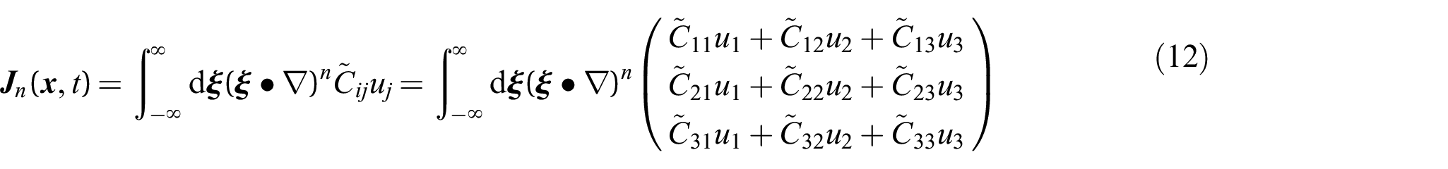
The governing equation of linear peridynamics can be written as (see also Silling [2])
where is the mass density, is the body force density, is the displacement vector, and
using the following property of the micromodulus :
In this paper, the micromodulus used in peridynamics is indicated with a tilde in order to distinguish the micromodulus from the stiffness matrix in classical elasticity introduced later. Let us set
Using the Taylor expansion, equation (5) can be rewritten as
Here, in equation (7), if necessary, the differential operators may be interpreted in the sense of pseudodifferential operators [44, 45]. Substituting equation (6) together with equation (7) into equation (1), we obtain the peridynamic equation as
Equation (8) is equivalent to the original equation (1) in the neighborhood of a material point , where is considered analytic, and this serves as a starting point for our investigation. We will investigate equation (8) for a certain class of micromoduli , and the focus will be on the asymptotic limit of equation (8) in the limit of the material horizon, , going to zero. The material horizon, , is a measure of the decay of the pairwise force density [2] of the peridynamic material, and is involved in the definition of the micromodulus . Strictly speaking, is the generalized material horizon defined in Mikata [1]:
where supp(•) denotes a support of a function [46, 47], and the maximum distance between a point and a set A is defined as
following a similar definition for the (minimum) distance between a point and a set [47]. Here is the standard Euclidean distance between two points and , and sup(•) denotes a supremum of a set. Thus, for a micromodulus with a finite support, the generalized material horizon is exactly the same as the original material horizon defined in Silling [2], by definition. Only for a micromodulus with an infinite support are they different: . We have chosen to be finite to handle a certain limiting process for a micromodulus with an infinite support.
since is an odd function of at least one variable of , and the integration domain is spherically symmetric with respect to the origin. Here ∇ is the del operator with respect to . Using equation (13) in equation (11), we obtain
We are interested in the peridynamic equation (equation (1)) in the limit of the generalized material horizon going to zero, . Substituting equation (14) into equation (1), we obtain
Taking the limit of the generalized material horizon, , in equation (15), we have
It can be shown that the following equation holds for an infinite number of micromoduli . The proof of this equation for triclinic materials is essentially the same as that for orthotropic materials given in Mikata [1], even though the matrix elements of become more involved.
Equation (18) represents the governing equation of linear peridynamics for any material system in the limit of the generalized material horizon going to zero, . In the following section, the asymptotic governing equation of linear peridynamics, equation (18), for triclinic materials will be discussed.
3. Triclinic peridynamic materials
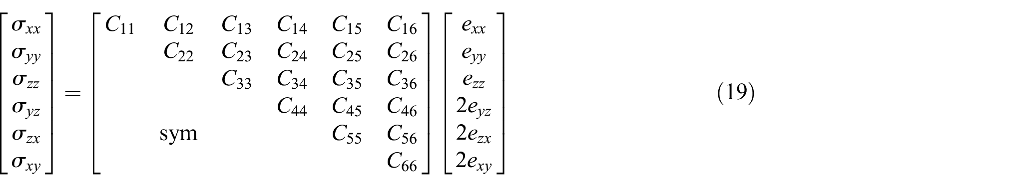
The goal of this section is to develop a peridynamic equation that represents the elastodynamic governing equation for triclinic materials in the limit of the generalized material horizon, δ, going to zero. In triclinic materials, the constitutive equation in the classical elasticity is given by [48]
with 21 independent elastic constants . The elastodynamic equilibrium equation and the strain displacement relation are given by, respectively,
When the material is isotropic, equation (22) reduces to the following Navier’s equation:
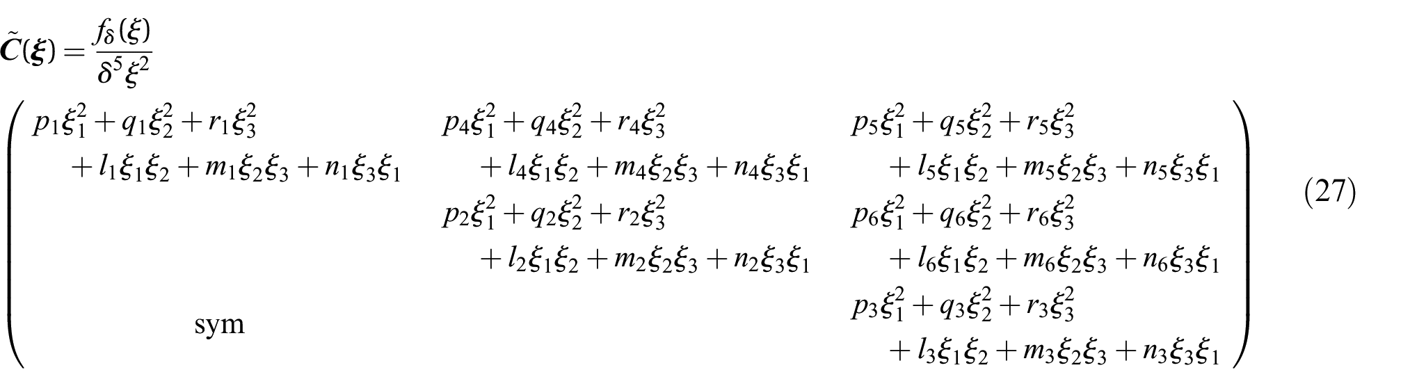
There may be an infinite number of peridynamic material models which represent the elastodynamic governing equation (22) in the limit of the generalized material horizon going to zero (). Let us obtain an infinite number of such peridynamic material models by considering the micromodulus of the following form:
where is a function of and , called a “nonlocality function”, which has to satisfy certain requirements [1], is the generalized material horizon given by equation (9), is the Kronecker delta, is a relative position vector, and , , , , , and (i = 1, …, 6) are the material constants to be determined, and
The only requirement for the nonlocality function is given by (see Mikata [1])
where
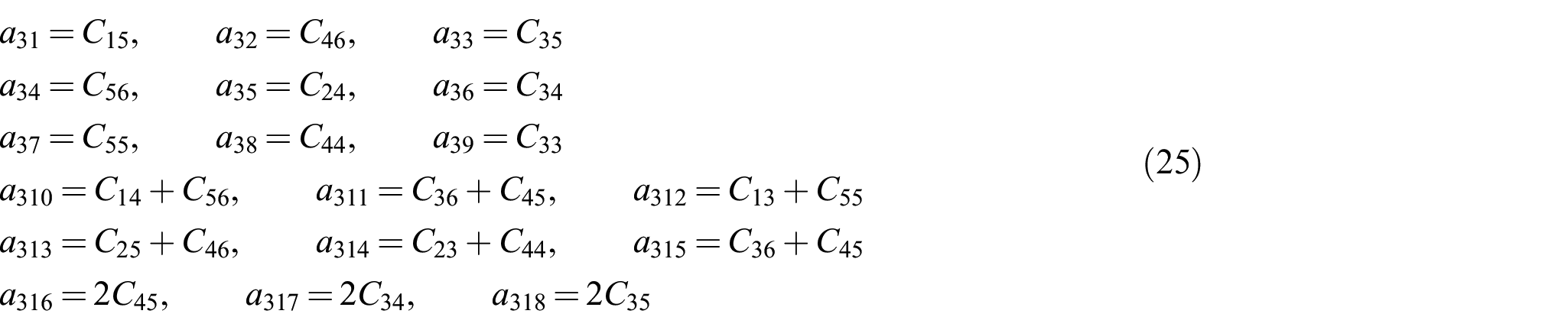
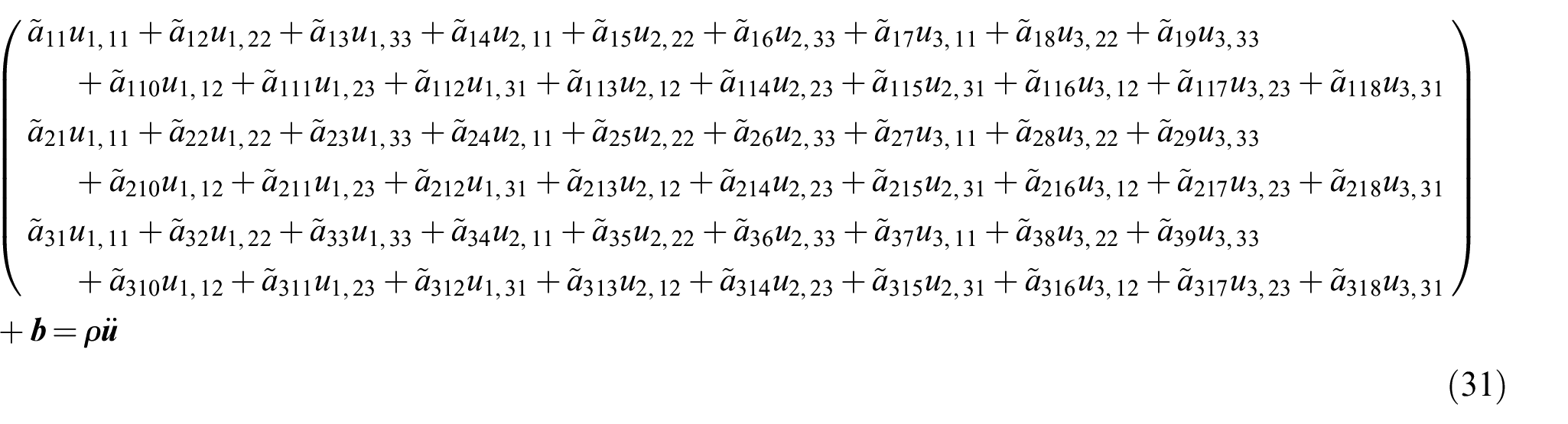
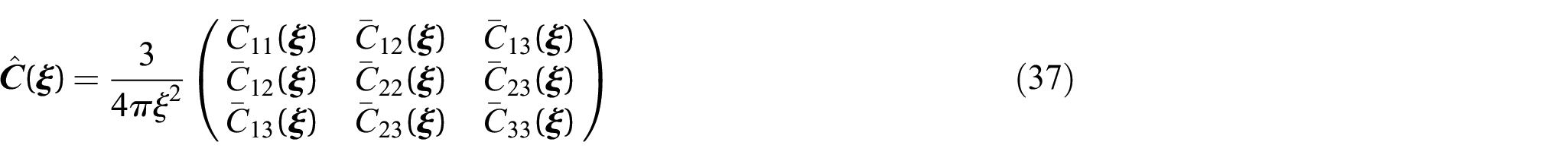
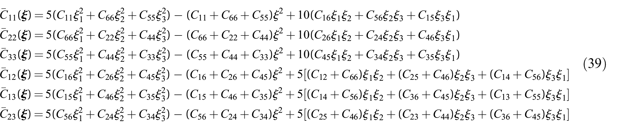
As can be seen from equation (27), the micromodulus needed for triclinic materials is significantly more involved than the one for orthotropic materials (see Mikata [1]). Substituting equation (27) into equation (18), we obtain
where the coefficients can be easily written as limits and integrals of micromoduli and polynomials of , but explicit expressions are not given here. For the elastodynamic governing equation (equation (22)) to be equivalent to the asymptotic peridynamic equation (equation (31)), the following set of equations has to hold:
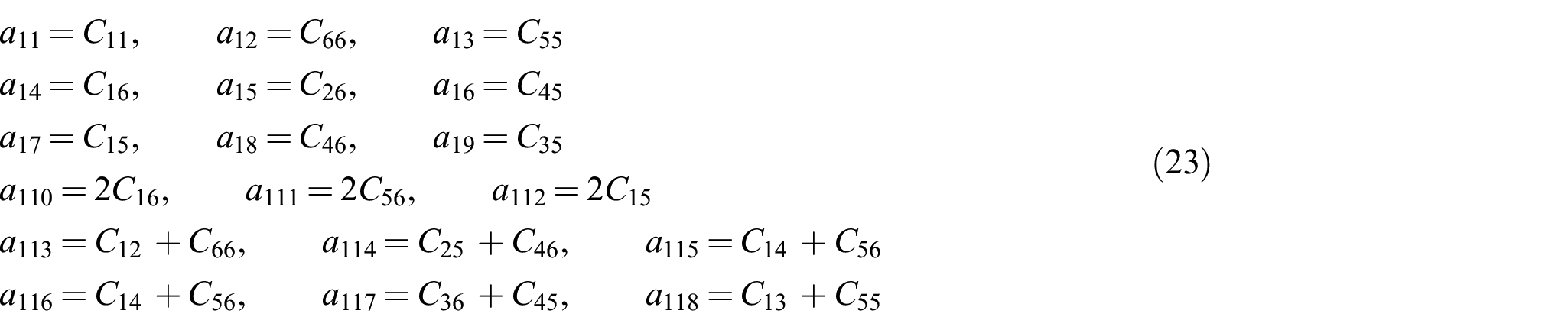
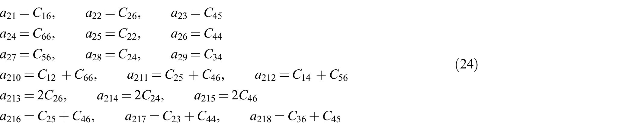
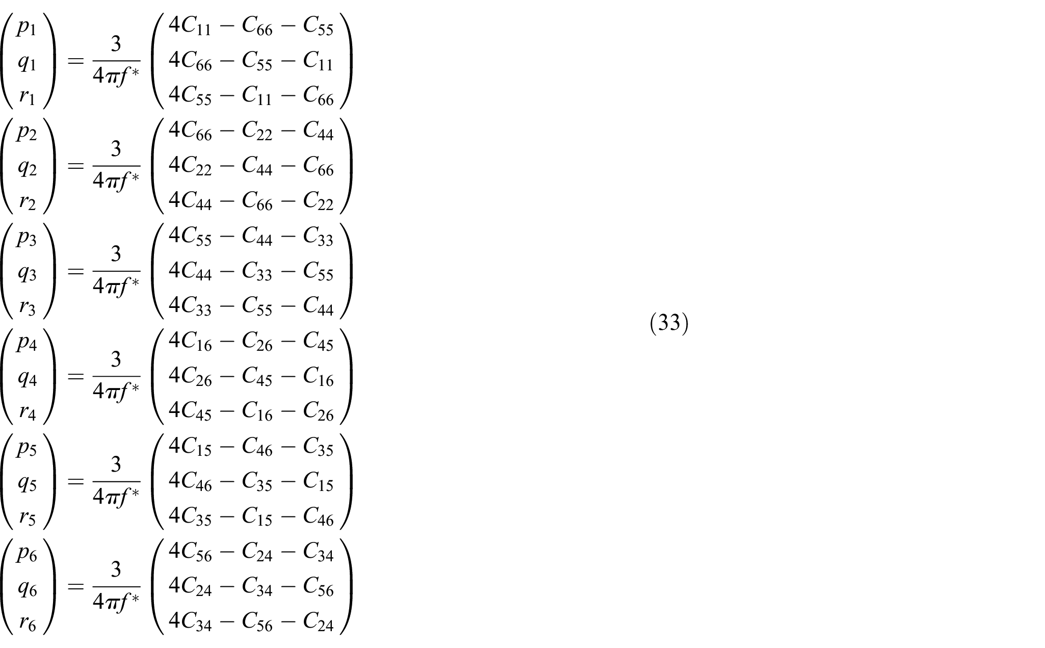
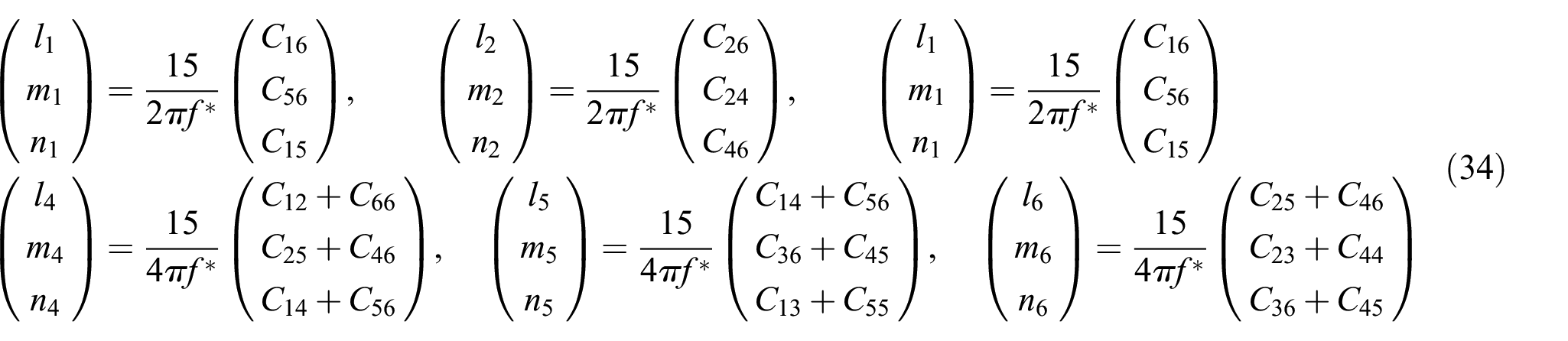
By using equations (23) to (25), together with the fact that the limit signs involved in are superfluous for the particular micromodulus given in equation (27), equation (32) can be rewritten without the limit sign. After examining the resulting equations, it can be seen that, out of 54 equations represented by equation (32), 18 equations are repeated. Therefore, equation (32) represents a system of 36 equations for 36 unknown constants , , , , , and (i = 1, …, 6) used for defining the micromodulus given in equation (27). Substituting equation (27) into the resulting equation obtained from equation (32), performing some algebra, and solving the resulting equation for the 36 unknown constants , , , , , and (i = 1, …, 6), we finally obtain
where is defined in equation (35), and is a nonlocality function, whose requirement is given by equation (29). Since there is an infinite number of nonlocality functions that satisfy the requirement, the micromodulus given in equation (36) represents an infinite number of micromoduli, which make the peridynamic equation (equation (1)) reduce to the elastodynamic equation (equation (22)) in the limit of the generalized material horizon going to zero, . It is noted in equation (36) that all the dependence of a micromodulus on a nonlocality function is contained in . The function is called a normalized nonlocality function. The reduction of the micromodulus given in equation (36) to the case of monoclinic and orthotropic materials is given in Appendix A.
4. Micromoduli with particular nonlocality functions
Different nonlocality functions produce different micromoduli. However, the dependence of a micromodulus on a nonlocality function is entirely contained in , as seen in equation (36). Furthermore, this function is common to all the material classes: triclinic, monoclinic, and orthotropic materials (see Appendix A). Therefore, in discussing the difference of the micromoduli that is due to a nonlocality function, we only need to discuss a normalized nonlocality function .
Let us consider a class of nonlocality functions defined by
where the function does not depend on the horizon . It should be mentioned here that the class of nonlocality functions defined by equation (40) is a subset of nonlocality functions satisfying equation (29), provided that
Examples of a normalized nonlocality function are given in the following:
Example 1:
Example 2:
Example 3:
It is clear from these examples that an infinite number of micromoduli can be generated, which make the peridynamic equation (equation (1)) reduce to the elastodynamic equation (equation (22)) in the limit of the generalized material horizon going to zero, .
5. Dispersion relations for triclinic peridynamic materials
Let us seek for a plane wave solution to the peridynamic governing equation (equation (1)) without the body force density. Let us set
where is an angular frequency, is a wave number, is a wave number vector, is a propagation unit vector, and is a displacement vector. Here we also have
Equation (48) is an eigenvalue problem for the angular frequency as a function of the wave number k, and the eigenvector determines the mode of the displacement vector . The relationship between k and defines the dispersion relation. Once is determined, an analytical solution to the peridynamic governing equation (equation (1)) without the body force density is given by equation (46).
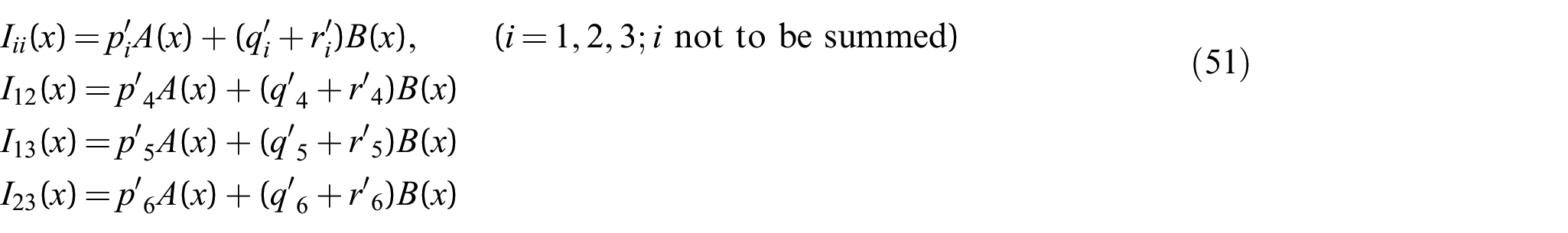
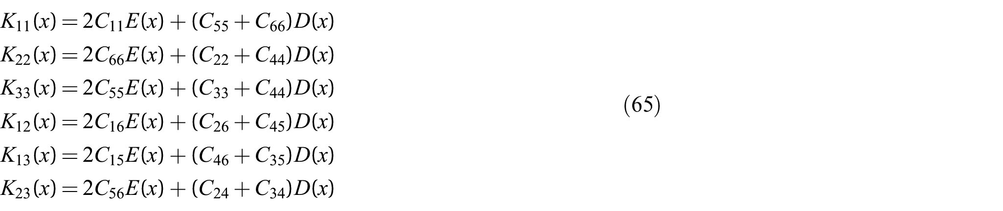
In this paper, we obtain the dispersion relations for the triclinic materials only for the propagation vector . Substituting equation (36) into equation (49), and performing some algebra, we obtain the following results:
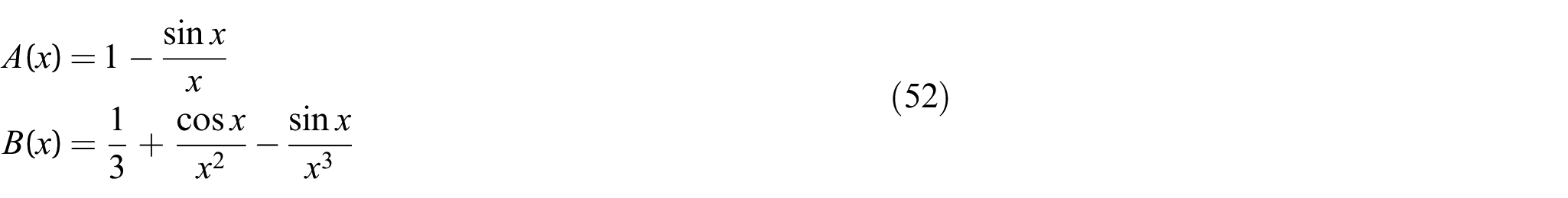
where
and
It should be mentioned here that and are the same functions as and in Mikata [1], respectively, and also the same functions as and in Silling [2], respectively. Let us write in Mikata [1] and in Silling [2] as . Then we have the following relation:
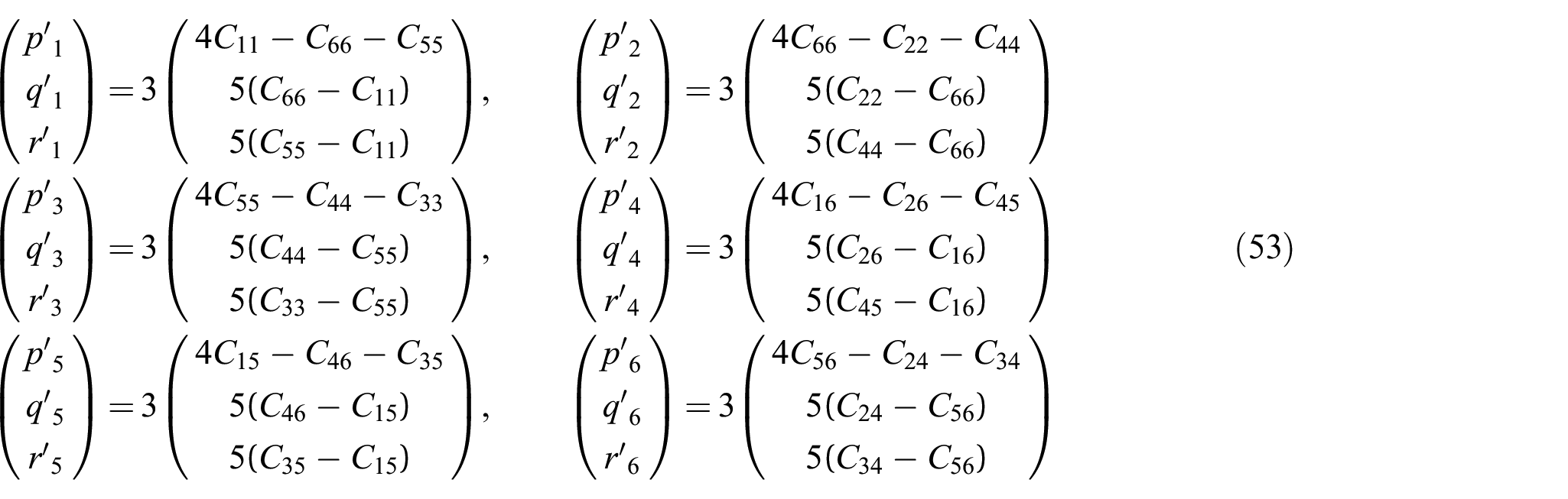
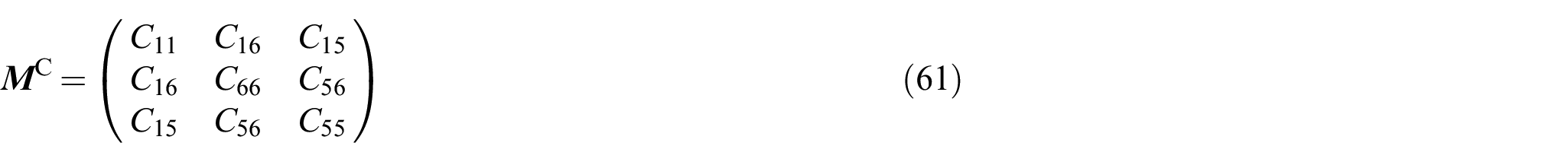
Using equation (48), the dispersion relations for the triclinic peridynamic materials for the propagation vector are obtained as
where (; ) are the eigenvalues of , which are defined by
and
In a similar manner to a plane wave solution (equation (46)) for a peridynamic triclinic material, we can seek for a plane wave solution of the governing equation (equation (22)) for a classical triclinic material. Let us set
where is a displacement vector for a classical triclinic material. The complete plane wave solution for a classical triclinic material is given in Appendix B. The corresponding dispersion relations for classical (nonperidynamic) triclinic materials are nondispersive, and those dispersion relations for the propagation vector are given by (see Appendix B)
where , , and are the wave speeds in classical triclinic materials, which correspond to one longitudinal wave and two transverse shear waves, respectively, and (; ) are the eigenvalues of , which are defined by
and
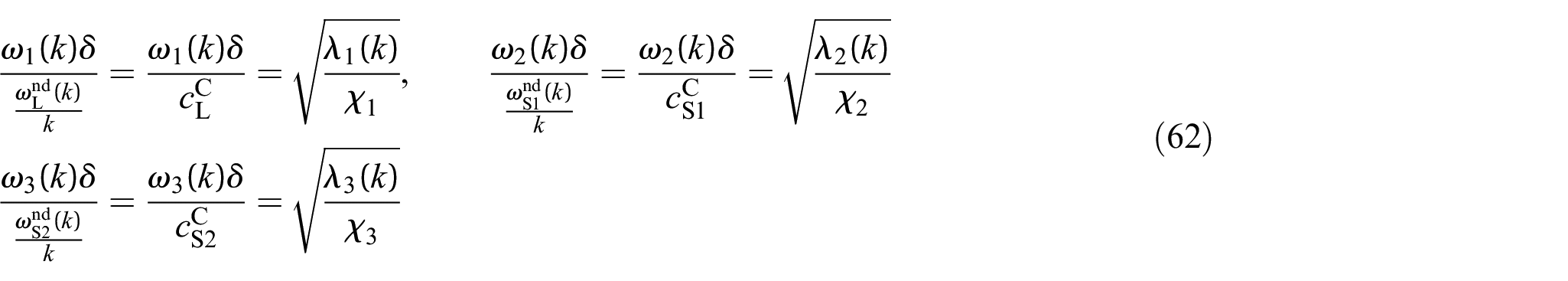
Using equations (55) and (59), nondimensionalized angular frequencies can be defined as
which can be plotted against a nondimensional wave number . Using equations (50) and (57), we have
where
and
It is noted here that , , , and are all bounded at as follows:
Specific dispersion curves are discussed in the next section.
6. Numerical results
Examples 1, 2, and 3 of the normalized nonlocality function, , listed in Section 4 are used to plot dispersion curves. From equations (43) to (45) and (64), we have:
Case A (Example 1):
Case B (Example 2):
Case C (Example 3):
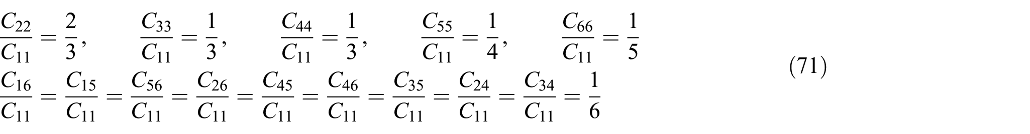
Numerical results are produced for the material with the following properties:
The micromodulus is given by equation (36). Therefore, a different normalized nonlocality function corresponds to a different peridynamic material.
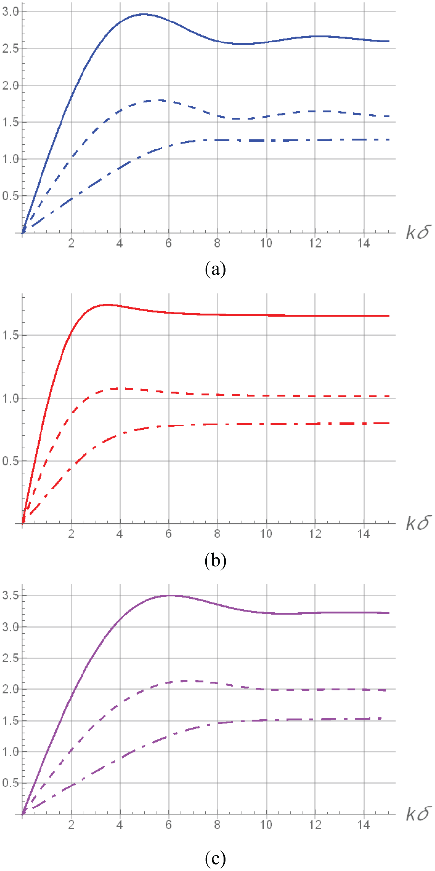
It should be noted here that Cases A and B correspond to Materials 1 and 2, respectively, in equation (109) of Silling [2], if the peridynamic material is isotropic and, furthermore, the Poisson ratio () is 0.25. As was mentioned in Mikata [1], 5 in the denominator of equation (109) for Material 2 in Silling [2] appears to be in error. For the triclinic material defined by equation (71), the normalized dispersion curves, , , and , are shown for Case A in Figure 1(a). Similarly, the normalized dispersion curves, , , and , are shown for Cases B and C in Figure 1(b) and (c), respectively. Let us call the waves corresponding to the eigenfrequencies , , wave 1, wave 2, and wave 3, respectively. Let us also note here that wave 1 corresponds to a longitudinal wave, and waves 2 and 3 correspond to transverse shear waves. It is seen from Figure 1 that, in higher frequency domains, i.e., approximately for Case A, for Case B, and for Case C, a group velocity, , of wave 1 and wave 2 becomes negative, which indicates anomalous dispersion. This was also reported in one-dimensional peridynamic wave propagation [33] and wave propagation in orthotropic peridynamic materials [1]. Dispersion of waves, group velocity, and anomalous dispersion are discussed, for example, in Achenbach [49], Brillouin [50], and Chu and Wong [51].
Normalized dispersion curves (solid line, longitudinal wave), (dashed line, shear wave), (dashed dot line, shear wave) as a function of for a triclinic peridynamic material: (a) Case A; (b) Case B; (c) Case C.
Normalized dispersion curves, , for Cases A, B, and C are shown in Figure 2(a). Similarly, normalized dispersion curves, and , for Cases A, B, and C are shown in Figure 2(b) and (c), respectively. It is seen from Figure 2 that, when the generalized material horizon approaches zero, all the normalized dispersion curves in each figure approach that of a nondispersive media, as expected:
Normalized dispersion curves for Cases A, B, and C as a function of in a triclinic peridynamic material, shown with a nondispersive solution (straight line) in the classical limit of the generalized material horizon : (a) ; (b) ; (c) .
This fact can also be shown mathematically. The general proof rests on the fact that the peridynamic governing equation (equation (1)) with equation (27) reduces to the governing equation of a regular triclinic material, equation (22), in the limit of the generalized material horizon going to zero (i.e., ). This can also be directly proven by showing that
the details of which are given in Appendix C. It is interesting to note that the behavior of the normalized dispersion curves, especially the relative ordering of the magnitude of dispersion curves, shown in Figure 2(a), is similar to the ones shown in Figure 8 of Mikata [33] and Figure 4 of Mikata [1]. In addition, it should be mentioned that there is a general similarity between the results (Figures 1 and 2) in this paper and the results (Figures 1 to 6) in Mikata [1]. This is because the material properties, equation (71) of this paper and equation (80) of Mikata [1], used in producing these results are similar except that , , , , , , , , and are nonzero in equation (71). If these constants are zero (), the two results would be identical.
In performing this limit of the constants going to zero (), where the constants are represented by , however, the procedure of plotting normalized dispersion curves becomes a little tricky, even though those cases are not shown in this paper. This is because the dispersion curves of two transverse waves (the two lower curves in Figure 1(a) and (c) start crossing each other at a particular wave number , when becomes less than a particular value, and the triclinic material starts approaching an orthotropic material. Since the eigenfrequencies , , and are defined numerically only through the relative order of their values (i.e., ) for a given wave number k, and not analytically, if we want to plot meaningful dispersion curves in those cases, it requires care. Let us set
Then it can be shown graphically that
where , , and are the angular frequencies of one longitudinal and two transverse waves in an orthotropic peridynamic material defined in Mikata [1]. The details are, however, not shown in this paper.
7. Conclusion
The governing equation of linear peridynamics is developed for triclinic materials (the most general anisotropic materials). As a departure from the standard peridynamic theory, the linear constitutive equation in the form of a micromodulus is determined by directly requiring the resulting peridynamic equation to converge to a comparable classical elastodynamic equation for a triclinic material as the generalized material horizon approaches zero. The methodology used in this paper follows closely that of Mikata [1], where linear peridynamics for up to orthotropic materials have been treated. However, the treatment of triclinic materials for peridynamics turns out to require a significantly more involved micromodulus compared with the case of orthotropic materials. Clearly, the formulation is different from that of either bond-based or state-based peridynamics as currently implemented. Nonetheless, it provides an explicit governing equation complete with a micromodulus, which is guaranteed to converge to that of classical elasticity as the material horizon approaches zero, regardless of the material anisotropy.
One of the benefits of the development in this paper is that the selection of the material model (i.e., the micromodulus) becomes systematic and straightforward for any anisotropic material. Also, when the material is orthotropic, the governing equation for orthotropic peridynamic materials obtained previously [1] is recovered as a special case from the governing equation for triclinic peridynamic materials obtained in this paper. As an example of a solution to the newly developed peridynamic governing equations for triclinic materials, a plane wave solution is analytically obtained for a triclinic peridynamic material, and dispersion curves are discussed. The governing peridynamic equations together with the micromodulus for triclinic materials developed in this paper can be used in a variety of peridynamic applications involving any anisotropic material.
One important modification made in this and the previous paper [1] regarding the material horizon [2] is the introduction of the generalized material horizon. The concept of the generalized material horizon is necessary to handle a certain limiting process, which is central to the new approach used in this and the previous paper [1]. As for the type of micromodulus, only the spherically symmetric micromodulus is considered.
Footnotes
Appendix A. Reduction to monoclinic and orthotropic materials
When the materials are monoclinic and orthotropic, the number of independent elastic constants becomes 13 and 9, respectively. Accordingly, among the 21 elastic constants appearing in the constitutive equation (equation (19)) for the triclinic material, there are several interrelations as follows.
Thus, we have recovered the main result (equation (47)) of Mikata [1]. Further reduction to the micromoduli for transversely isotropic, cubic, and isotropic peridynamic materials is discussed in Mikata [1].
Appendix B. Plane wave solution for classical triclinic materials
Equation (22) without the body force can be written as
Thus, the angular frequency for a wave with a propagation vector and a wave number is given by
where is defined by the following eigenvalue problem:
Appendix C. Asymptotic expression for M P and its consequences
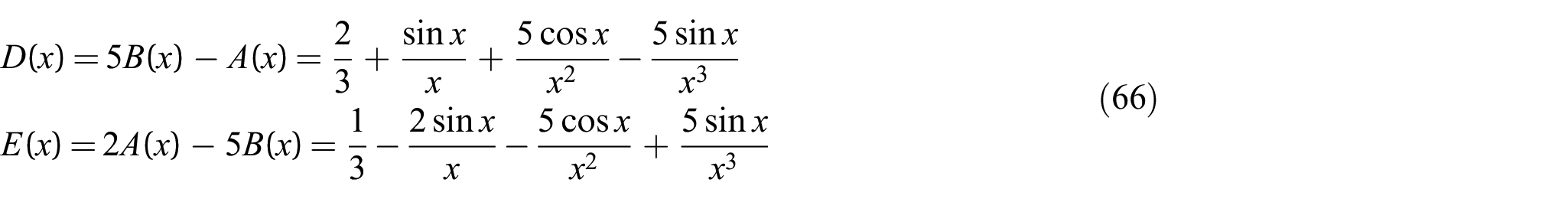
The goal of this appendix is to prove equation (72) by showing the asymptotic expression (equation (73)) in the limit of a generalized material horizon going to zero (i.e., ). Taylor expansions of D(x) and E(x) in equation (66) are given by
KrönerE.On the physical reality of torque stresses in continuum mechanics. Int J Eng Sci1963; 1: 261–278.
6.
KrönerE.Elasticity theory of materials with long range cohesive forces. Int J Solids Struct1967; 3: 731–742.
7.
KrönerE. Interrelations between various branches of continuum mechanics. In: KrönerE (ed.) Generalized mechanics of continua. Berlin: Springer-Verlag, 1968, 330–340.
8.
KrönerEDattaBK.Nichtlokale Elastostatik: Ableitung aus der Gittertheorie. Z Phys1966; 196: 203–211.
9.
KuninIA.Elastic media with microstructure I: One-dimensional models. Berlin: Springer-Verlag, 1982.
10.
KrumhanslJA. Some considerations of the relation between solid state physics and generalized continuum mechanics. In: KrönerE (ed.) Generalized mechanics of continua. Berlin: Springer-Verlag, 1968, 298–311.
11.
KuninIA. The theories of elastic media with microstructure and the theory of dislocations. In: KrönerE (ed.) Generalized mechanics of continua. Berlin: Springer-Verlag, 1968, 321–329.
12.
VaismanAMKuninLA.Boundary value problems in nonlocal theory of elasticity. J Appl Math Mech1969; 33: 765–777.
13.
EringenAC.Nonlocal polar elastic continua. Int J Eng Sci1972; 10: 1–16.
14.
EringenAC.Linear theory of nonlocal elasticity and dispersion of plane waves. Int J Eng Sci1972; 10: 425–435.
15.
EringenACEdelenGDB. On nonlocal elasticity. Int J Eng Sci1972; 10: 233–248.
16.
RogulaD.Introduction to nonlocal theory of material media. In: RogulaD (ed.) Nonlocal theory of material media (CISM Courses and Lectures, vol. 268). Vienna: Springer Verlag, 1982, 125–222.
17.
Di PaolaMFaillaGZingalesM. The mechanically-based approach to 3D nonlocal elasticity theory: Long-range central interactions. Int J Solids Struct2010; 47: 2347–2358.
18.
ZingalesM.Wave propagation in 1D elastic solids in presence of long-range central interactions. J Sound Vib2011; 330: 3973–3989.
19.
LubineauGAzdoudYHanF, et al. A morphing strategy to couple non-local to local continuum mechanics. J Mech Phys Solids2012; 60: 1088–1102.
20.
Di PaolaMFaillaGPirrottaA, et al. The mechanically based non-local elasticity: An overview of main results and future challenges. Philos Trans R Soc London, Ser A2013; 371: 20120433.
21.
KhodabakhshiPReddyJN.A unified integro-differential nonlocal model. Int J Eng Sci2015; 95: 60–75.
22.
SillingSAZimmermannMAbeyaratneR.Deformation of a peridynamic bar. J Elast2003; 73: 173–190.
23.
WecknerOAbeyaratneR.The effect of long-range forces on the dynamics of a bar. J Mech Phys Solids2005; 53: 705–728.
24.
SillingSAAskariE.A meshfree method based on the peridynamic model of solid mechanics. Comput Struct2005; 83: 1526–1535.
25.
GerstleWSauNSillingS.Peridynamic modeling of concrete structures. Nucl Eng Des2007; 237(12–13): 1250–1258.
26.
DemmiePNSillingSA.An approach to modeling extreme loading of structures using peridynamics. J Mech Mater Struct2007; 2(10): 1921–1945.
27.
WecknerOAskariAXuJ, et al. Damage and failure analysis based on peridynamics – theory and applications. In: 48th AIAA/ASME/ASCE/AHS/ASC Structures, Structural Dynamics, and Materials Conference, 2007.
28.
AskariEBobaruFLehoucqRB, et al. Peridynamics for multiscale materials modeling. J Phys Conf Ser2008; 125: 012078.
29.
KilicBMadenciE.Structural stability and failure analysis using peridynamic theory. Int J Non Linear Mech2009; 44: 845–854.
30.
HaYDBobaruF.Studies of dynamic crack propagation and crack branching with peridynamics. Int J Fract2010; 162: 229–244.
31.
BobaruFDuangpanyaM.The peridynamic formulation for transient heat conduction. Int J Heat Mass Transfer2010; 53: 4047–4059.
32.
SillingSAWecknerOAskariE, et al. Crack nucleation in a peridynamic solid. Int J Fract2010; 162: 219–227.
33.
MikataY.Analytical solutions of peristatic and peridynamic problems for a 1D infinite rod. Int J Solids Struct2012; 49: 2887–2897.
34.
De MeoDDiyarogluCZhuN, et al. Modeling of stress-corrosion cracking by using peridynamics. Int J Hydrogen Energy2016; 41: 6593–6609.
35.
WangLAbeyaratneR.A one-dimensional peridynamic model of defect propagation and its relation to certain other continuum models. J Mech Phys Solids2018; 116: 334–349.
36.
MikataY.Peridynamics for heat conduction. J Heat Transfer2020; 142: 081402.
37.
ParksMLLehoucqRBPlimptonSJ, et al. Implementing peridynamics within a molecular dynamics code. Comput Phys Commun2008; 179(11): 777–783.
38.
GalvanettoUMudricTShojaeiA, et al. An effective way to couple FEM meshes and peridynamics grids for the solution of static equilibrium problems. Mech Res Commun2016; 76: 41–47.
39.
MadenciEOterkusE.Peridynamic theory and its applications. New York: Springer, 2014.
40.
SillingSAEptonMWecknerO, et al. Peridynamic states and constitutive modeling. J Elast2007; 88: 151–184.
41.
WarrenTLSillingSAAskariA, et al. A non-ordinary state-based peridynamic method to model solid material deformation and fracture. Int J Solids Struct2009; 46: 1186–1195.
42.
GhajariMIannucciLCurtisP.A peridynamic model for the analysis of dynamic crack propagation in orthotropic media. Comput Methods Appl Mech Eng2014; 276: 431–452.
43.
AguiarAR.On the determination of a peridynamic constant in a linear constitutive model. J Elast2016; 122: 27–39.
44.
Gel’fandIMShilovGE.Generalized functions, vol. 2: Spaces of fundamental and generalized functions. New York: Academic Press, 1968.
45.
HörmanderL.The analysis of linear partial differential operators, vol. III: Pseudo-differential operators. Berlin: Springer, 1985.
46.
Gel’fandIMShilovGE.Generalized functions, vol. 1: Properties and operations. New York: Academic Press; 1964.
47.
HaaserNBSullivanJA.Real analysis. New York: Dover Publications, 1991.
48.
LekhnitskiiSG.Theory of elasticity of an anisotropic elastic body. San Francisco: Holden-Day, 1963.
49.
AchenbachJD.Wave propagation in elastic solids (Applied Mathematics and Mechanics, vol. 16). Amsterdam: North-Holland. 1973.
50.
BrillouinL.Wave propagation and group velocity. New York: Academic Press, 1960.
51.
ChuSWongS.Linear pulse propagation in an absorbing medium. Phys Rev Lett1982; 48: 738–741.