
Abstract
We propose an anisotropic and nonlinear generalization of the Kelvin–Voigt viscoelastic model obtained considering the additive splitting of the Cauchy stress tensor in an elastic and a dissipative part. The former one corresponds to a fiber-reinforced hyperelastic material while the dissipative effect is described by the most general linear transverse-isotropic tensorial function of symmetric part of the velocity gradient. In a such a way we characterize the dissipative contribution via three viscoelastic moduli. We then show, by a detailed analysis of the simple shear quasistatic motion and the corresponding creep phenomena, that this motion may be used to determine experimentally the viscoelastic parameters.
1. Introduction
A basic model of viscoelasticity is due to Kelvin and Voigt and, from a rheological point of view, it consists of a spring and a damping element that are parallel to each other [1]. Since this model superposes the elastic and the viscous behavior, it is quite simple to generalize it to a nonlinear setting and this has been done for isotropic elastic materials by many authors (see, for example, Antman and Malek-Madani [2], Destrade and Saccomandi [3], and the discussion in Destrade et al. [4].
To understand this procedure, let us consider the motion

A possible generalization of the Kelvin–Voigt model in a nonlinear setting is obtained splitting the Cauchy stress tensor,

where

where
In the context of the polymers and soft tissue mechanics, it is often necessary to consider anisotropic models. For example, this is the case of thermoplastic composites [5] or biomechanics of ligaments [6]. It is therefore natural to ask how it is possible to obtain a version of the Kelvin–Voigt model suitable for the nonlinear and anisotropic context.
If we consider a material reinforced with one family of fibers, the representation formula for the stress tensor of a material such that
To make real progress at this point, it is necessary to make simplifying assumptions a priori. For example, in Anssari-Benam et al. [8], a model to investigate uniaxial tensile deformation tests of porcine aortic valve specimens at various deformation rates is investigated. The dissipative part of the constitutive equation proposed in Anssari-Benam et al. [8] depends linearly only on two invariants via a dissipation potential. Another simplification is proposed in O’Callaghan et al. [9] and in Destrade and Saccomandi [19]. This last paper is devoted to the study of travelling shear waves in the special model:

where:


These simplifications of the general theory are not dictated by a rational methodology of investigation but only by empirical considerations or computational simplifications. A compromise between the complexity of the general theory in Merodio [7] and the specificity of the various particular models as in Anssari-Benam et al. [8] or Destrade and Saccomandi [10] may be indicated by the isotropic model (1), i.e., by the mix between the classic theory of hyperelasticity and the Navier–Stokes theory.
We remind that the Navier–Stokes theory is obtained requiring “the most general linear isotropic function

where
Using this result, it is natural to consider an anisotropic Kelvin–Voigt model, that for the sake of algebraic simplicity, we restrict here to a strain-energy density in the form
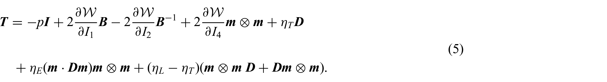
This model is the transverse isotropic version of equation (1) and is characterized only by three viscous parameters.
The aim of this paper is to investigate if shearing motions and specifically the classical recovery experiment based on the simple shear motion in the quasistatic setting are sufficient to determine these three viscosity parameters. In such a way, we have a clear control of the most general transverse incompressible isotropic viscoelastic model of differential type linear in the second-order tensor
The plan of this paper is as follows. In section 2, we write down the basic equations of the problem, and, in section 3, we investigate into details the simple shear motions showing that indeed it is possible to use the recovery experiment to determine the three viscous moduli. The final section 4 is devoted to concluding remarks.
Our aim is to use the same strategy that Ray Ogden and co-workers (see, for example, Merodio and Ogden [15]) used to investigate anisotropic nonlinear elastic media: we start with a simple model to build up step by step a clear understanding of what to expect in the context of a mechanical behavior that often defies our induction. For this reason, we would like to dedicate this study to Ray, a great gentleman and great scientist, but above all a great friend and esteemed collaborator.
2. Basic equations
Let us consider the following class of isochoric motions:

such that

We compute:

However, since:

we have:

i.e.,

The equation of motion in absence of body forces is:

where

From the first two equations in equation (7), we obtain:

where
Being

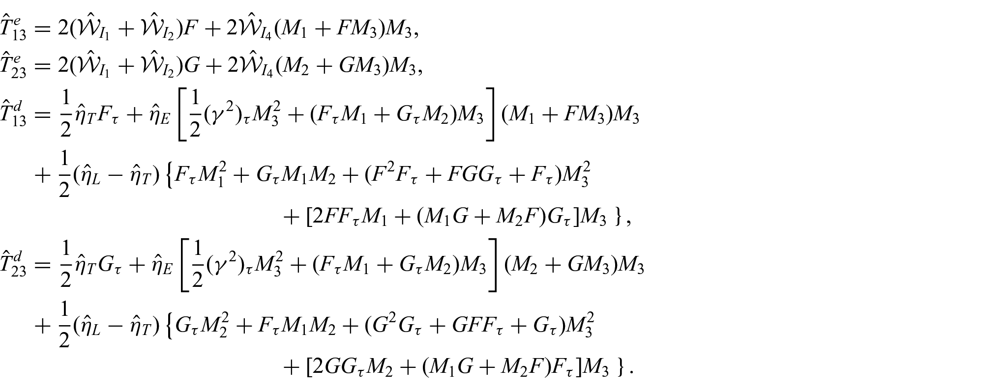
and the dimensionless stresses:

where
Using the dimensionless variables and the notation

where:

and:
Here,

are the dimensionless “viscosities”.
It is of fundamental importance to note that:

When we consider the strain-energy associated with the standard linear solid (3), we have that the elastic part of the stress tensor is simplified as:


where
For the sake of simplicity, in the following, we will use for the elastic part the standard linear solid (3), and this because the elastic part is usually determined by a static experiment and here we wish to focus on the viscoelastic part of the constitutive equation. The use of more general hyperelastic form of the strain-energy has a minor impact on our results.
The system (8) is a third-order nonlinear highly coupled system of partial differential equations in the unknown
and nontrivial solutions of equation (8) are possible if and only if
It is interesting to consider
In the next section, we will restrict our attention to the quasistatic limit of equations (8), i.e., when

An important solution of this set of equations is obtained considering
We point out that the quasistatic limit is meaningful only when a global existence theorem for the solutions of equations (8) may be ensured [16], but this is still an open problem also for the general differential viscoelastic model in the isotropic case.

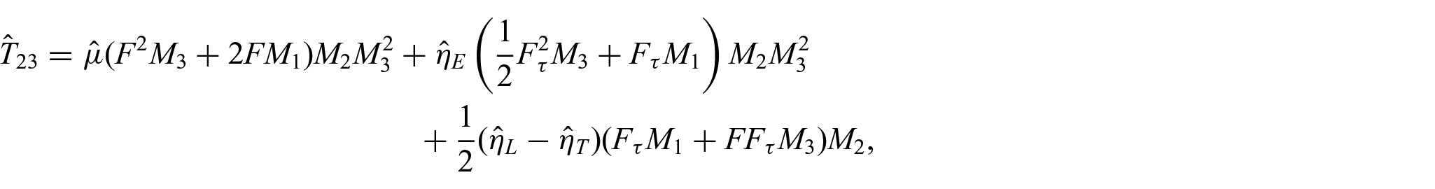
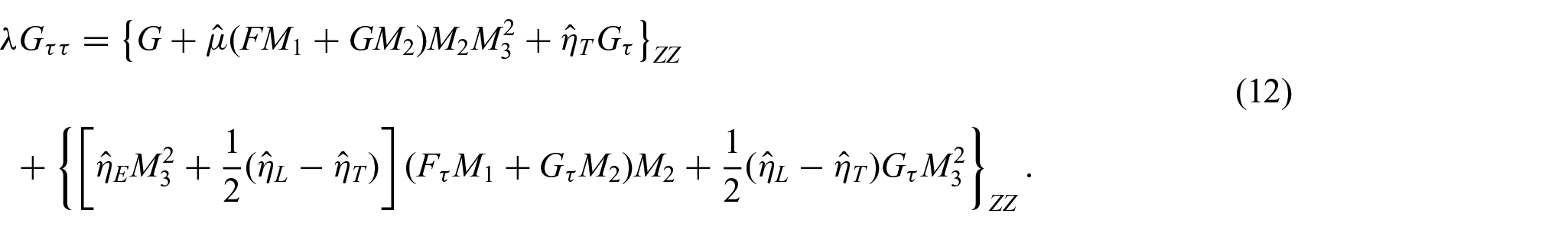
where

So, it is clear that our model is dissipative. We remark that equation (14) is a quadratic form in the variables

whose components are functions of
3. Simple shear
The simple shear motions are fundamental to investigate the characteristic viscoelastic phenomena of creep and recovering.
Let us focus on the creep experiment. We remind that for an isotropic linear material, if we have the stress history

We point out that, in this case, it must be
3.1. Linear anisotropic case
Now, let us consider the same problem in the case of the linear but anisotropic situation.
We consider once again the stress history:

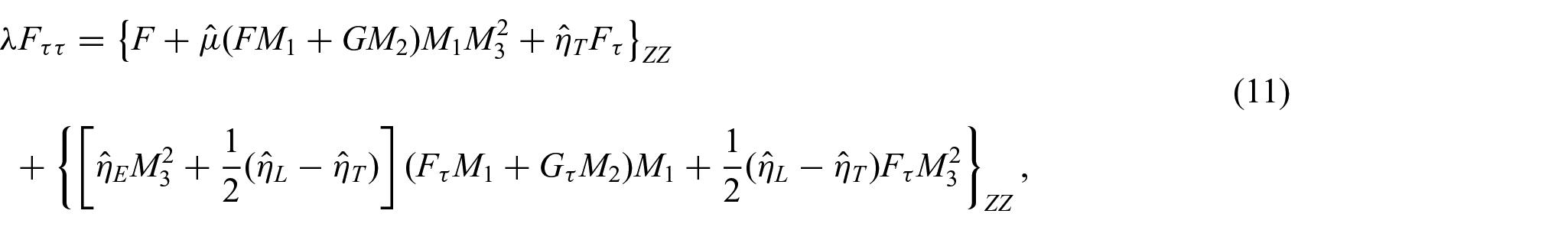
But now, at least in the general case, equation (13) is not decoupled and, therefore, we have to solve the system:

subject to

When

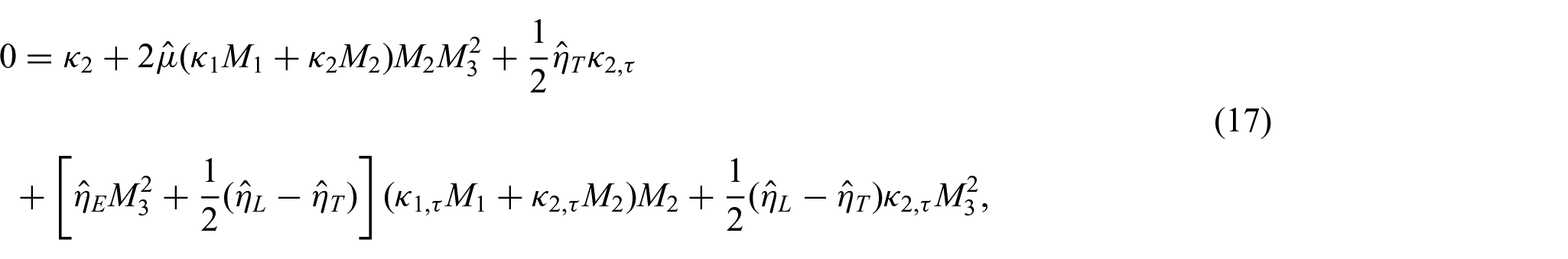
where, since

and:

With the representation
Equations (16) and (17) decouple also in the case

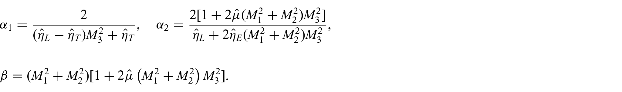
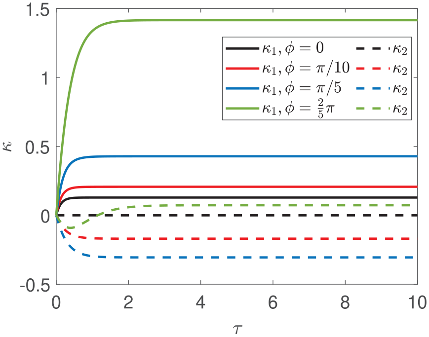
The general solution of the first-order system of the linear ordinary differential equations (16) and (17) is easy to obtain and reads as follows:
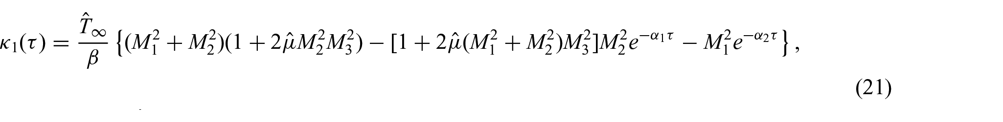

where:
Clearly,
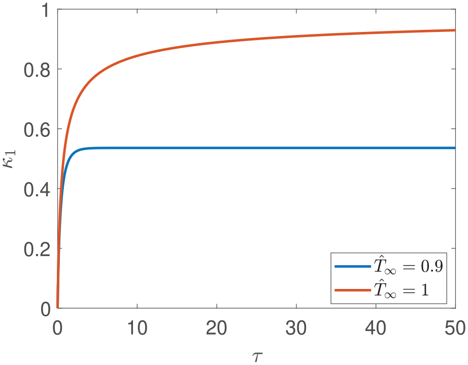
Using the representation
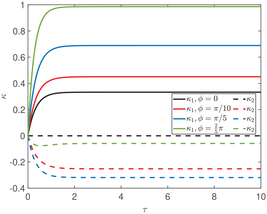
Plot of
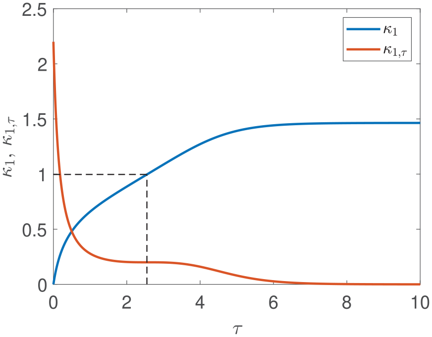
In Figure 2, we show in more detail the non-monotonic behavior of

we have that
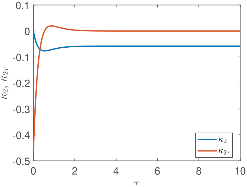
Plot of
These solutions are interesting because they show in a simple direct way that, when
The solutions (18) and (20) and the general solution of the systems (16) and (17) show that by considering appropriate angles between the direction of the fiber and the shear strain, we have sufficient information to determine experimentally the various viscosity coefficients.
3.2. Nonlinear anisotropic case
The nonlinear case is clearly more complex. In the isotropic case, this problem has been considered into details in Pucci and Saccomandi [19]. Here, we analyze first the situation when the system (13) decouples to point out the possible “pathologies” of the anisotropic case, and then we give a condition to avoid such pathologies for a generic arrangement of the fibers.
3.3. Case
To decouple equation (13), we set
To simplify the notation, we choose the characteristic time

and:

where:

We point out that, because of the requirement (14), it must be
The BVP to solve for the recovery phenomena is given by:

Here,

We remind, without loss of generality, that we choose
The differential equation in this BVP problem may be solved by quadrature as:

The following theorem is fundamental for our analysis.

the solution
The hypothesis in equation (25) ensures that the algebraic solution

Indeed, for
The problem is that, given a strain-energy density, the conditions (25) may be not guaranteed for all the directions

the roots of:

are given by:

where:

and the roots in equation (28) are real so that the monotony of
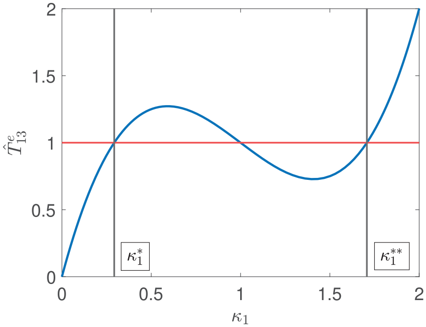
For this reason, it is fundamental to consider the sign of
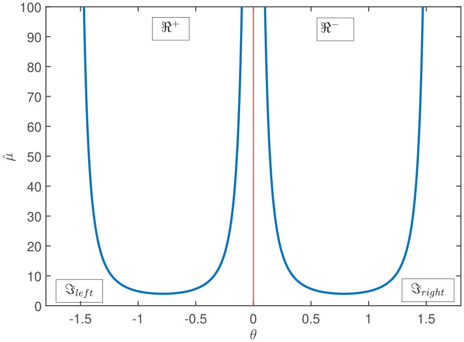
Plot of
However, when we are in the regions
The problems arise only if we are in the region

and it is clear that we enter the region
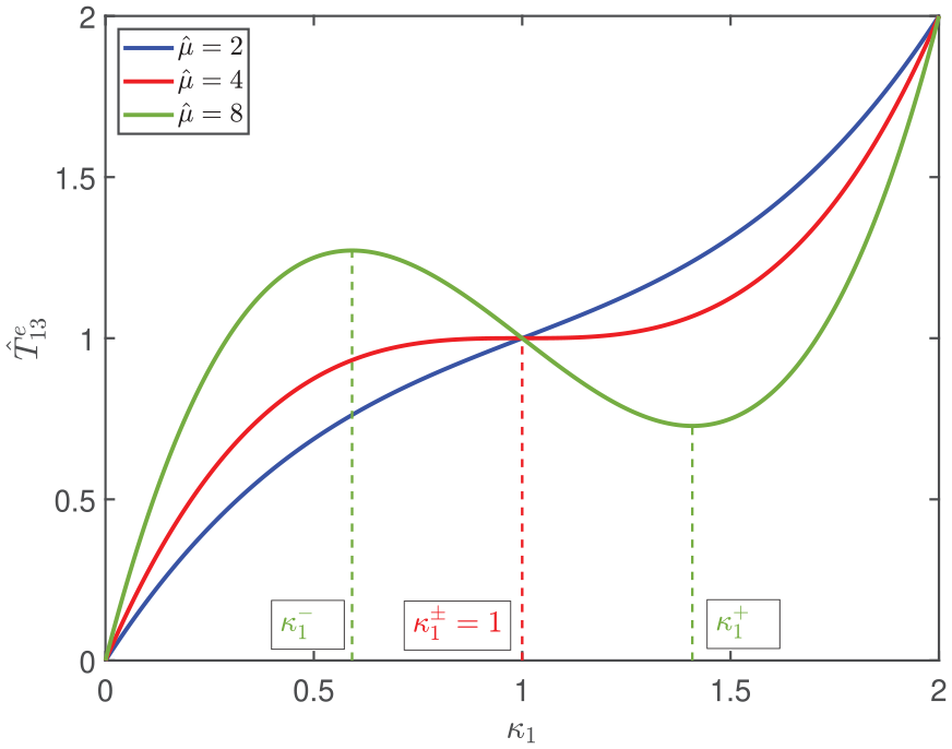
Plot of
For
For the last choice, i.e.,

therefore, we note a non-monotonic behavior and our theorem it is no more valid.
To understand how it is possible to solve the BVP (22) in the non-monotonic case, it is interesting to analyze in more details the borderline case

is characterized by a unique algebraic solution
Plot of the creep solution
It is therefore possible to apply our theorem, but we point out that when
The next step is to increase the applied shearing stress to a value
Plot of the creep solution
The previous solution is helpful to understand what happens to the creep solution when we contradict the first of the requirements in equation (25) as in the case
In Figure 7, we plot
Plot of the Maxwell line for
In Figure 7, we note that the Maxwell line intersects
If we consider
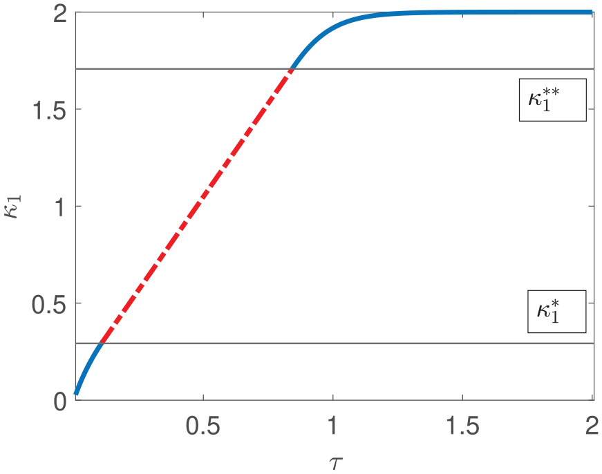
Solution of equation (22) when
It is important to note that in the non-monotonic situation, the solution is no more analytic.
However, in a soft device [21], it is possible also to consider that the amount of shear
This example shows what is going on when our theorem cannot be applied. It is clear that in an experiment designed to measure the viscosity moduli it is reasonable to avoid these, theoretically interesting, but, in some sense, “exotic” phenomena and therefore to choose angles between the shear direction and the fibers away from the region
3.4. General fiber direction
Having analyzed in detail the reasons that can mathematically lead pathologies, it is now possible to treat the general case in such a way as to avoid these problems.
When
First, we have to ensure the uniqueness of the solution of the system:

Using the relationship (9), this uniqueness is guaranteed by assuming the positive definiteness of the Hessian matrix of the strain-energy function

Second, we have to rewrite the equation (13) as:

Since the matrix

The functions
Therefore, under the hypotheses (14) and (30), we may use, as we have done in the linear case, the creep experiment to characterize the viscosity moduli in the nonlinear context in a direct and safe way, and, clearly, the method we have here outlined may be applied to any general strain-energy density
The solution of the nonlinear system (8) is shown in Figure 9, for which the same parameters of the linear case considered in Figure 1 are used. We point out that the linear and nonlinear cases are qualitatively similar.
Plot of
4. Concluding remarks
We have presented a nonlinear model of viscoelasticity that is the strict analogue for the case of a transversely isotropic solid of the basic Kelvin–Voigt isotropic model (1). Moreover, we have shown that the classical recovery experiment in a simple shear quasistatic deformation is sufficient to experimentally measure the three viscous parameters that characterize the model (5) we have proposed.
Once again, we have made clear that in continuum mechanics an accurate rheological model of the complex mechanical behavior of materials cannot be done without laying its foundations on a robust understanding of hyperelasticity. Indeed, the possibility of using experimental tests based on simple shear motions depends substantially on the behavior of the elastic part of the Cauchy stress tensor. This fact supports Alan Wineman’s point of view [24]: “An education in nonlinear elasticity means that one is also educated, though perhaps unaware of it, in the foundations of several additional subjects.”
It is believed that the model proposed here can be a starting point for a more rigorous analysis of the nonlinear viscoelasticity of anisotropic materials. In fact, in the current literature, the choice of the numerous constitutive functions that appear in the completely general theory is made empirically and arbitrarily. In our model, however, one can still aspire to have control of the various dissipative parts of the Cauchy stress tensor, and it is possible to have a clear understanding of the possibility of certain simplifications of equation (5). For example, when we study thermoplastic composites, it is usual to consider the reinforcing fibers as inextensible [5]. In this framework, it is therefore possible to set the extensional viscosity
Other opportunities for model (5) may be obtained considering the viscoelastic parameters as functions of the various invariants. In so doing, we may be able to capture, e.g., strain rate effects in the viscosities. However, one must be very careful when considering these generalizations because the good mathematical position of these models even in the quasistatic case can be quite complex [26]. Finally, it must be remembered that the Kelvin–Voigt model cannot describe the stress-relaxation phenomena typical of many polymeric models, but it is not hard to use equation (5) to generalize to an anisotropic framework a model like the one proposed in Filograna et al. [27].
For all these reasons, we think that the model proposed here has a great potential to be applied in various contexts where it is necessary to describe the mechanical behavior of anisotropic polymeric materials or soft tissues.
Footnotes
Acknowledgements
The authors were supported by Gruppo Nazionale per la Fisica Matematica (GNFM) of the Istituto Nazionale di Alta Matematica (INdAM). G.S. acknowledges the financial support of Istituto Nazionale di Fisica Nucleare through IS “Mathematical Methods in Non-Linear Physics,” Prin Project 2017KL4EF3 and Fondo di Ricerca di Base of Unipg. M.C. acknowledges the INdAM-GNFM Progetto Giovani 2023 “P-systems in non linear elastodynamics” (E53C22001930001) and the financial support from project FSE REACT-EU, Asse IV—Istruzione e ricerca per il recupero, Azione IV.6—Contratti di ricerca su tematiche Green, DM 1062 del 10-08-2021, “Modelli fisico matematici per lo studio e la simulazione di sistemi e prodotti eco-sostenibili basati su nuovi materiali.”
Funding
The author(s) received no financial support for the research, authorship, and/or publication of this article.