Analysis of a new kind of elastic-rigid bilateral obstacle problem

Abstract

This paper is devoted to a study of a new kind of bilateral obstacle problem. The obstacles are made of rigid bodies covered by soft layers which are deformable and allow penetration. A model of an elastic rigid bilateral obstacle problem is established, and three equivalent descriptions are derived: the energy form, the variational inequality form, and the differential equation form. We prove the solution existence and uniqueness of this model and provide an error estimate of the numerical solutions. The optimal order error estimate for the linear finite element method is derived under the proper regularity assumption. A penalty method is introduced to solve the finite element approximation problem, and the convergence results are obtained when the penalty parameter tends to infinity. Several numerical examples are reported, and the results are in good agreement with the theoretical analysis.

Keywords

Bilateral obstacle problem finite element method variational inequality error estimates numerical analysis

1. Introduction

The obstacle problem is a typical variational inequality of the first kind, which appears in the fields of physics, financial management science, engineering applications, etc. [1]. This problem has attracted much attention from scholars because of its inherent mathematical theory and wide applications. In the past decades, mathematical theories and numerical analysis of this model have been established extensively and thoroughly. For more details, we recommend the works by Ran and Cheng [1], Bouchlaghem and Mermri [2, 3], Duvaut and Lions [4], Hoppe [5], Imoro [6], Kärkkäinen [7], Kinderlehrer and Stampacchia [8], Kornhuber[9, 10], Murea and Tiba [11, 12], Ran et al. [13], Rodrigues [14], Tarvainen [15], and Yuan and Cheng [16].

In classical obstacle models, the obstacle is perfectly rigid. However, there are no perfectly rigid bodies in practice. Small penetrations could occur, due to the body’s and foundation’s asperities [17]. A new kind of elastic-rigid unilateral obstacle problem is proposed in the work by Cheng et al. [18], in which the obstacle is made of a rigid body covered by a soft layer. Inspired by the work by Cheng et al. [18], we consider a new kind of elastic-rigid bilateral obstacle model. More precisely, the elastic membrane is constrained to lie between two obstacles which are made of rigid bodies covered by layers made of soft material.

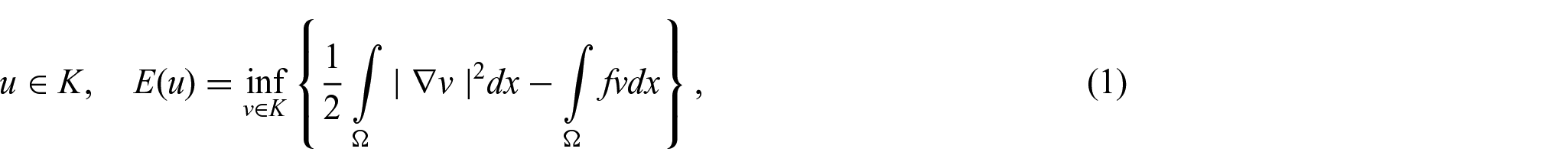
The classical bilateral obstacle problem can be described as follows: assume that the elastic membrane (1) is a homogeneous membrane occupying a domain $Ω$ ; (2) lies between a lower obstacle of height $ϕ$ and a upper obstacle of height $ψ$ ; (3) is equally stretched in all directions by a uniform tension and loaded by a normal uniformly distributed force $f$ [16]. Let $u$ be the vertical displacement component of the membrane. According to the principle of minimum energy, the displacement $u$ satisfies

u \in K, E (u) = inf_{v \in K} {\frac{1}{2} \int_{Ω} | \nabla v |^{2} dx - \int_{Ω} fvdx},

(1)

where $K = {v \in H_{0}^{1} (Ω) | ϕ \leq v \leq ψ, a . e . in Ω}$ is a feasible set; $Ω \subset R^{d}$ is a bounded domain with Lipschitz boundary $\partial Ω$ ; $ϕ$ and $ψ$ satisfy $ϕ \leq ψ \in H^{1} (Ω) \cap C (Ω)$ with $ϕ |_{\partial Ω} \leq 0$ and $ψ |_{\partial Ω} \geq 0$ .

It is well known that equation (1) has the equivalent form:

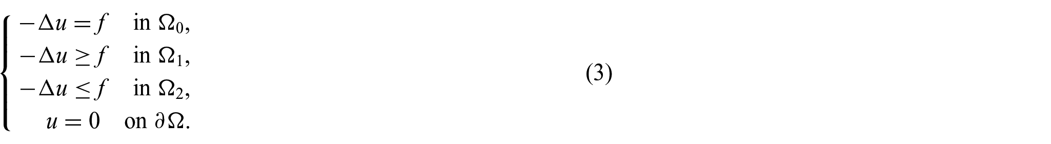
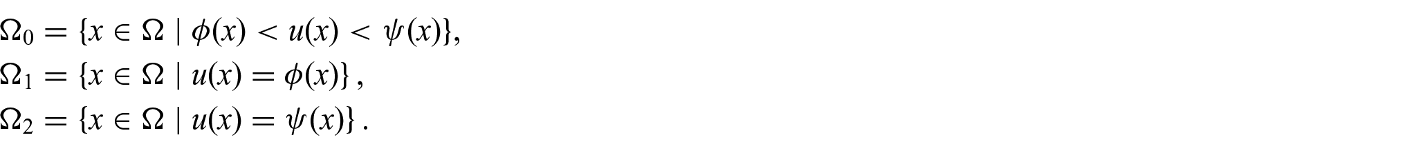
u \in K, \int_{Ω} \nabla u \cdot \nabla (v - u) dx \geq \int_{Ω} f (v - u) dx, \forall v \in K,

(2)

If the solution $u \in C^{2} (Ω) \cap H_{0}^{1} (Ω)$ , the variational inequality (2) also can be transformed to the differential equation form

{\begin{matrix} - Δ u = f in Ω_{0}, \\ - Δ u \geq f in Ω_{1}, \\ - Δ u \leq f in Ω_{2}, \\ u = 0 on \partial Ω . \end{matrix}

(3)

where

\begin{matrix} Ω_{0} = {x \in Ω | ϕ (x) < u (x) < ψ (x)}, \\ Ω_{1} = {x \in Ω | u (x) = ϕ (x)}, \\ Ω_{2} = {x \in Ω | u (x) = ψ (x)} . \end{matrix}

For more details, we refer to the works by Ran et al. [13], Yuan and Cheng [16], and Glowinski [19].

In this paper, we consider the elastic-rigid foundation in the bilateral obstacle problem of the elastic membrane. More precisely, the upper obstacle and the lower obstacle are both made of rigid bodies covered with soft layers. The soft layers are deformable and allow penetration, so the elastic membrane will be subject to the corresponding normal reaction pressure during the penetration process. In section 2, we establish a new elastic-rigid bilateral obstacle model and prove the existence and uniqueness result. We also derive three equivalent forms. In section 3, we consider numerical approximations. The optimal-order error estimate is obtained. In section 4, we give four numerical examples to support our theoretical analysis. Finally, the content of this paper is summarized in the last section.

2. The new bilateral obstacle problem

First, let us introduce the symbols to be used, $H^{1} (Ω)$ denotes the Sobolev space $W^{1, 2} (Ω)$ with the usual norm, $H_{0}^{1} (Ω)$ the closure of $C_{0}^{\infty} (Ω)$ in $H^{1} (Ω)$ , and $H^{- 1} (Ω)$ the dual space of $H_{0}^{1} (Ω)$ ; the dual pairing between $H_{0}^{1} (Ω)$ and $H^{- 1} (Ω)$ is denoted by 〈.,.〉. $∥ \cdot ∥_{X}$ is the norm on the norm space X, and $(\cdot, \cdot)_{Y}$ is the inner product on the Hilbert space $Y$ and simply write (·,·) when there is no confusion. $Δ$ refers to the Laplace operator, and ∇ the gradient operator.

Let $f \in L^{2} (Ω)$ , non-negative function $g_{1}, g_{2} \in H^{1} (Ω)$ and $ϕ \leq ψ \in H^{1} (Ω) \cap C (Ω)$ with $ϕ \leq 0, ψ \geq 0$ on $\partial Ω$ . We consider the following problem: under the action of a vertical force $f$ , find the equilibrium position of the elastic membrane clamped on the boundary of $Ω$ , and the elastic membrane will be constrained by the bilateral obstacles, with the height of $ϕ$ and $ψ$ , respectively. Where the bilateral obstacles are covered by soft layers with thickness of $g_{1}$ and $g_{2}$ , respectively, and the soft layers are deformable and allow penetration. Therefore, the elastic membrane will be subject to the reactive normal pressure of the soft layer during the contact process.

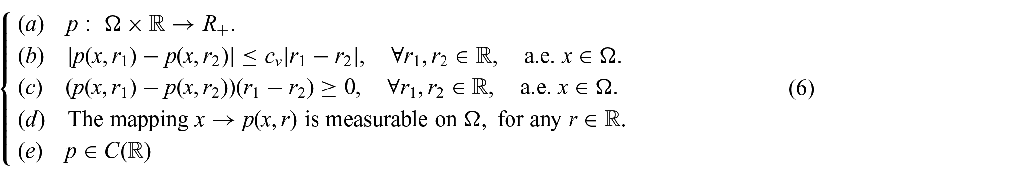
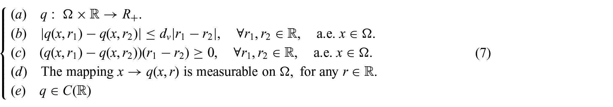
The reaction pressure of an elastic membrane subjected to a soft layer is very important. Many normal reaction pressure functions have been defined in many publications. Here, we consider a commonly used function (see, e.g. [20 –22]). Define $p, q$ : $R \to R$ by

p (r) = {\begin{matrix} c_{v} {[r]}_{+}, & if r < η, \\ c_{v} η, & if r \geq η, \end{matrix}

(4)

q (r) = {\begin{matrix} d_{v} {[r]}_{+}, & if r < ξ, \\ d_{v} ξ, & if r \geq ξ, \end{matrix}

(5)

where $[r]_{+} = \max {r, 0}$ and the constant $c_{v}, d_{v} \geq 0$ are stiffness coefficient. $η, ξ \geq 0$ are two constants determined by the specific problem. Obviously, the functions $p$ and $q$ satisfy:

{\begin{matrix} (a) p : Ω \times R \to R_{+} . \\ (b) | p (x, r_{1}) - p (x, r_{2}) | \leq c_{v} | r_{1} - r_{2} |, \forall r_{1}, r_{2} \in R, a . e . x \in Ω . \\ (c) (p (x, r_{1}) - p (x, r_{2})) (r_{1} - r_{2}) \geq 0, \forall r_{1}, r_{2} \in R, a . e . x \in Ω . \\ (d) The mapping x \to p (x, r) is measurable on Ω, for any r \in R . \\ (e) p \in C (R) \end{matrix}

(6)

and

{\begin{matrix} (a) q : Ω \times R \to R_{+} . \\ (b) | q (x, r_{1}) - q (x, r_{2}) | \leq d_{v} | r_{1} - r_{2} |, \forall r_{1}, r_{2} \in R, a . e . x \in Ω . \\ (c) (q (x, r_{1}) - q (x, r_{2})) (r_{1} - r_{2}) \geq 0, \forall r_{1}, r_{2} \in R, a . e . x \in Ω . \\ (d) The mapping x \to q (x, r) i s measurable on Ω, for any r \in R . \\ (e) q \in C (R) \end{matrix}

(7)

and then we get the normal reactive pressure expressed as follows:

p (ϕ - u) = {\begin{matrix} c_{v} {[ϕ - u]}_{+}, & if ϕ - u < g_{1}, \\ c_{v} g_{1}, & if ϕ - u \geq g_{1}, \end{matrix}

and

q (u - ψ) = {\begin{matrix} d_{v} {[u - ψ]}_{+}, & if u - ψ < g_{2}, \\ d_{v} g_{2}, & if u - ψ \geq g_{2} . \end{matrix}

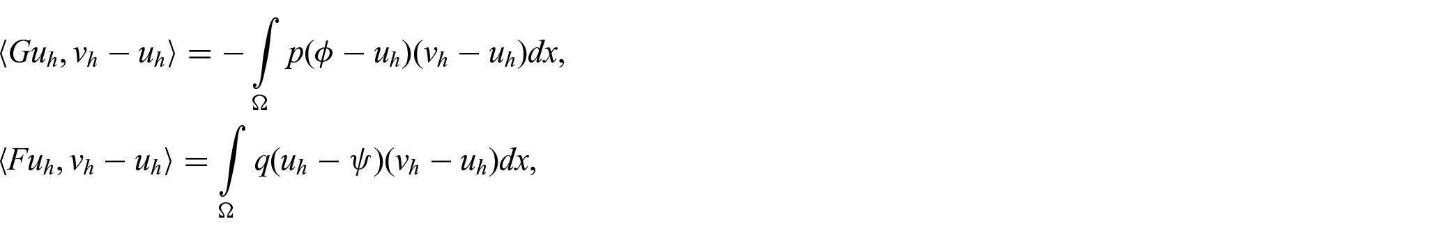
In fact, for each point $x$ , if $ϕ (x) < u (x) < ψ (x)$ , the elastic membrane has the normal reaction pressure as 0. When the penetration of the elastic membrane through the soft layers exceeds $g_{1}$ and $g_{2}$ , the soft layers of the obstacles offer no additional resistance to penetration. Using the Riesz’ representation theorem, we define two operators $G, F : H_{0}^{1} (Ω) \to H^{- 1} (Ω)$ and by the equality:

〈 Gu, v 〉 = - \int_{Ω} p (ϕ - u) vdx, \forall u, v \in H_{0}^{1} (Ω),

(8)

〈 Fu, v 〉 = \int_{Ω} q (u - ψ) vdx, \forall u, v \in H_{0}^{1} (Ω) .

(9)

According to the property of $p$ , $q$ shown in (6) and (7), it is easy to obtain that $G$ and $F$ are two monotone Lipschitz continuous operators.

Like the basic assumption and discussion in the work by Rodrigues [14], we can define the total potential energy of the elastic membrane as follows:

E (u) = \frac{1}{2} a (u, u) + j (u) + d (u) - (f, u) .

(10)

Here, $j (u) = \int_{Ω} \int_{u}^{ϕ} p (ϕ - τ) d τ dx$ and $d (u) = \int_{Ω} \int_{ψ}^{u} q (τ - ψ) d τ dx$ represent the normal reactive pressure when the elastic membrane passes through the soft layers, and

a (u, v) = \int_{Ω} \nabla u \cdot \nabla vdx, \forall u, v \in H_{0}^{1} (Ω) .

It is easy to verify that $a (u, v)$ is bounded and coercive. In fact, with the Cauchy–Schwarz inequality, there exists a constant $β_{1} > 0$

| a (u, v) | \leq β_{1} ∥ u ∥_{H^{1} (Ω)} ∥ v ∥_{H^{1} (Ω)}, \forall u, v \in H_{0}^{1} (Ω),

using the Poincaré–Friedrichs inequality, there exists a constant $β_{2} > 0$ such that

a (u, u) = | u |_{H^{1} (Ω)}^{2} \geq β_{2} ∥ u ∥_{H^{1} (Ω)}^{2}, \forall u \in H_{0}^{1} (Ω) .

According to the minimum energy principle of mechanics, the elastic membrane is stable at the equilibrium position $u$ when the total energy reaches the minimum, i.e.

u \in K, E (u) = inf_{v \in K} E (v),

(11)

where $K = {v \in H_{0}^{1} (Ω) | ϕ - g_{1} \leq v \leq ψ + g_{2}, a . e . in Ω}$ is the admissible displacement.

Theorem 1. The problem (11) has a unique solution.

Proof. Since $p$ and $q$ are continuous and nondecreasing, we can easily get that $j$ and $d$ are two convex and proper lower semicontinuous functions over $H_{0}^{1} (Ω)$ [19]. From the expression of $E$ , then we can deduce that $E$ is lower semicontinuous and strictly convex. Therefore, assuming that $K$ is bounded, we immediately get the conclusion according to the Weierstrass theorem in the work by Sofonea and Matei [22]. If $K$ is not bounded, since $a$ is coercive, it follows that

E (v) \geq \frac{β_{2}}{2} ∥ v ∥_{H^{1} (Ω)}^{2} + j (v) + d (v) - (f, v), \forall v \in K .

(12)

Then, using Proposition 1.29 in the work by Sofonea and Matei [22] and Riesz’ representation theorem, we know that there exist $l_{1}, l_{2} \in H_{0}^{1} (Ω)$ and $α_{1}, α_{2} \in R$ such that

j (v) \geq (l_{1}, v) + α_{1}, \forall v \in K .

(13)

d (v) \geq (l_{2}, v) + α_{2}, \forall v \in K .

(14)

Combining (12)–(14) and using Cauchy–Schwarz inequality, we immediately obtain that $E$ is coercive. Similarly, according to the Weierstrass theorem in the work by Sofonea and Matei [22], the problem (11) has a unique solution. □

Next, we show that the solution of problem (11) is equivalent to the following variational inequality:

u \in K, a (u, v - u) + 〈 Gu, v - u 〉 + 〈 Fu, v - u 〉 \geq (f, v - u), \forall v \in K .

(15)

Theorem 2. An element $u \in K$ is a solution to problem (11) if and only if it satisfies variational inequality (15).

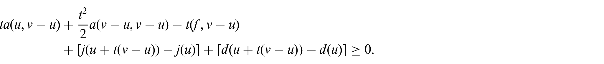
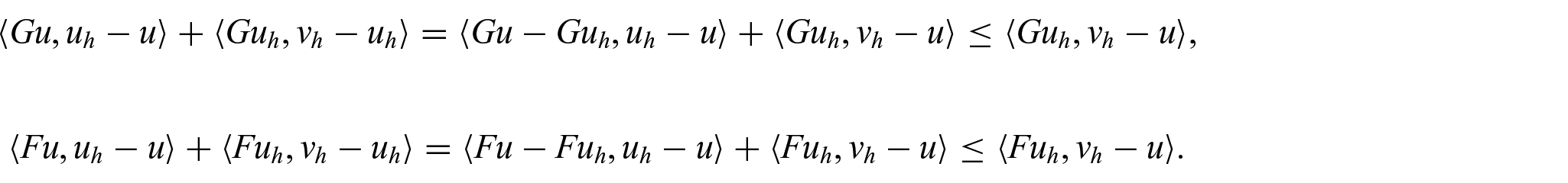
Proof. If $u \in K$ is a solution to problem (11), and let $t \in (0, 1)$ , we have

E (u) \leq E (u + t (v - u)), \forall v \in K,

then according to the definition of $E$ , we obtain

\begin{matrix} ta (u, v - u) + \frac{t^{2}}{2} a (v - u, v - u) - t (f, v - u) \\ + [j (u + t (v - u)) - j (u)] + [d (u + t (v - u)) - d (u)] \geq 0 . \end{matrix}

Divide the above inequality by $t > 0$ and let $t \to 0^{+}$ ; by the differential mean value theorem, we immediately obtain:

a (u, v - u) + 〈 Gu, v - u 〉 + 〈 Fu, v - u 〉 \geq (f, v - u), \forall v \in K .

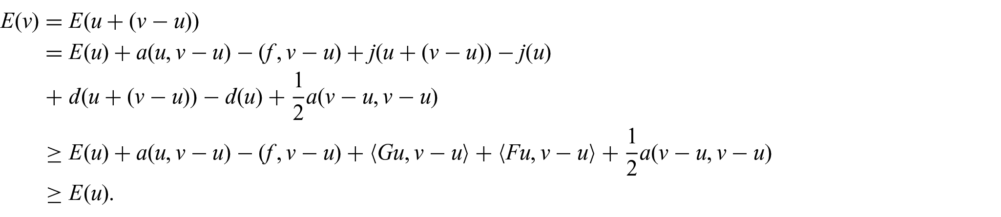
Conversely, if $u$ satisfies the variational inequality (15), i.e.

a (u, v - u) + 〈 Gu, v - u 〉 + 〈 Fu, v - u 〉 - (f, v - u) \geq 0, \forall v \in K .

Since both $j$ and $d$ are convex, namely

\begin{matrix} j (u + t (v - u)) - j (u) \leq (1 - t) j (u) + tj (v) - j (u) = t (j (v) - j (u)), \\ d (u + t (v - u)) - d (u) \leq (1 - t) d (u) + td (v) - d (u) = t (d (v) - d (u)) . \end{matrix}

We have $j (v) - j (u) \geq 〈 Gu, v - u 〉$ , $d (v) - d (u) \geq 〈 Fu, v - u 〉$ . Then, by the definition of $E$ , for any $v \in K$ satisfies:

\begin{matrix} E (v) = E (u + (v - u)) \\ = E (u) + a (u, v - u) - (f, v - u) + j (u + (v - u)) - j (u) \\ + d (u + (v - u)) - d (u) + \frac{1}{2} a (v - u, v - u) \\ \geq E (u) + a (u, v - u) - (f, v - u) + 〈 Gu, v - u 〉 + 〈 Fu, v - u 〉 + \frac{1}{2} a (v - u, v - u) \\ \geq E (u) . \end{matrix}

Therefore, $u \in K$ is the solution of problem (11). □

Now we have proved that the problem (11) is equivalent to the variational inequality form (15). Here, we use a similar discussing procedure as in the work by Ciarlet [23]. Assume that $f, ϕ, ψ, g_{1}, g_{2}$ all belong to $C (Ω)$ , and $u \in H^{2} (Ω) \cap H_{0}^{1} (Ω)$ , then we get the following result.

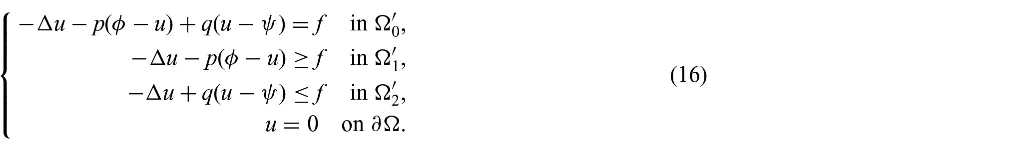
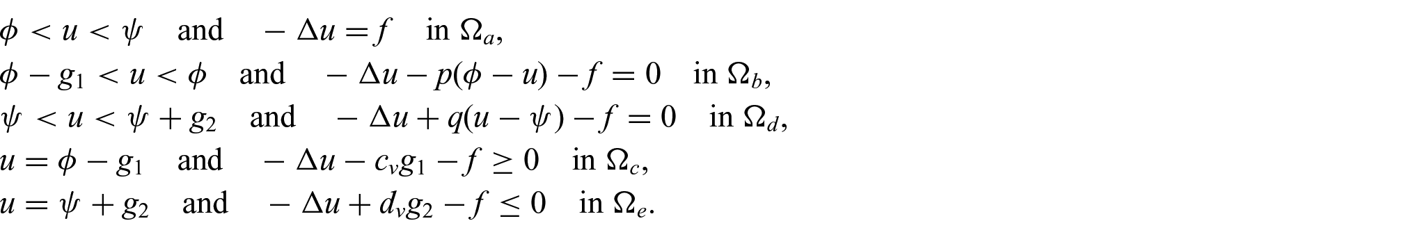
Theorem 3. If $u \in H^{2} (Ω) \cap H_{0}^{1} (Ω)$ is the solution of variational inequality (15), then $u$ satisfies

{\begin{matrix} - Δ u - p (ϕ - u) + q (u - ψ) = f in {Ω^{'}}_{0}, \\ - Δ u - p (ϕ - u) \geq f in {Ω^{'}}_{1}, \\ - Δ u + q (u - ψ) \leq f in {Ω^{'}}_{2}, \\ u = 0 on \partial Ω . \end{matrix}

(16)

where

\begin{matrix} {Ω^{'}}_{0} = {x \in Ω | ϕ (x) - g_{1} (x) < u (x) < ψ (x) + g_{2} (x)}, \\ {Ω^{'}}_{1} = {x \in Ω | u (x) = ϕ (x) - g_{1} (x)}, \\ {Ω^{'}}_{2} = {x \in Ω | u (x) = ψ (x) + g_{2} (x)} . \end{matrix}

Conversely, if $u \in C^{2} (Ω) \cap C (\bar{Ω})$ satisfies (16), then $u$ must be a solution of variational inequality (15).

Proof. Assume $u \in H^{2} (Ω) \cap H_{0}^{1} (Ω)$ is the solution of variational inequality (15). For some $x_{0} \in Ω$ satisfying $ϕ (x_{0}) - g_{1} (x_{0}) < u (x_{0}) < ψ (x_{0}) + g_{2} (x_{0})$ , then there exists a neighborhood $U (x_{0}) \subset Ω$ and a positive number $δ$ such that

ϕ (x) - g_{1} (x) + δ < u (x) < ψ (x) + g_{2} (x) - δ, \forall x \in U (x_{0}) .

For any $φ \in C_{0}^{\infty} (U (x_{0}))$ satisfying $∥ φ ∥_{\infty} \leq 1$ , applying variational inequality (15) with $v = u \pm δ φ$ and performing integration by parts yield:

\pm δ \int_{Ω} (- Δ u - p (ϕ - u) + q (u - ψ) - f) φ dx \geq 0, \forall φ \in C_{0}^{\infty} (U (x_{0})), ∥ φ ∥_{\infty} \leq 1 .

That is,

\int_{Ω} (- Δ u - p (ϕ - u) + q (u - ψ) - f) φ dx = 0, \forall φ \in C_{0}^{\infty} (U (x_{0})), ∥ φ ∥_{\infty} \leq 1 .

Then, we further get the following:

\int_{Ω} (- Δ u - p (ϕ - u) + q (u - ψ) - f) φ dx = 0, \forall φ \in C_{0}^{\infty} (U (x_{0})) .

Therefore, if $ϕ (x_{0}) - g_{1} (x_{0}) < u (x_{0}) < ψ (x_{0}) + g_{2} (x_{0})$ , $x_{0} \in Ω$ , we have

(- Δ u - p (ϕ - u) + q (u - ψ) - f) (x_{0}) = 0

i.e. $u$ must satisfy

- Δ u - p (ϕ - u) + q (u - ψ) = f, in Ω_{0}^{'} .

For some $x_{1} \in Ω$ satisfying $u (x_{1}) = ϕ (x_{1}) - g_{1} (x_{1})$ , then there exists a neighborhood $U (x_{1}) \subset Ω$ such that

u (x) = ϕ (x) - g_{1} (x), \forall x \in U (x_{1}) .

For any $φ \in C_{0}^{\infty} (U (x_{1}))$ that satisfies $0 \leq φ \leq ψ + g_{2} - (ϕ - g_{1})$ , taking $v = u + φ$ in variational inequality (15) and performing integration by parts, we obtain:

\int_{Ω} (- Δ u - p (ϕ - u) + q (u - ψ) - f) φ dx \geq 0, \forall φ \in C_{0}^{\infty} (U (x_{1})), 0 \leq φ \leq ψ + g_{2} - (ϕ - g_{1}) .

Then, we further get the following:

\int_{Ω} (- Δ u - p (ϕ - u) + q (u - ψ) - f) φ dx \geq 0, \forall φ \in C_{0}^{\infty} (U (x_{1})), φ \geq 0 .

Therefore, if $u (x_{1}) = ϕ (x_{1}) - g_{1} (x_{1})$ , $x_{1} \in Ω$ , we have

(- Δ u - p (ϕ - u) + q (u - ψ) - f) (x_{1}) \geq 0

i.e.

- Δ u - p (ϕ - u) + q (u - ψ) - f \geq 0, in Ω_{1}^{'} .

If $u = ϕ - g_{1}$ , we have $u - ψ = (ϕ - g_{1}) - ψ < 0 < g_{2}$ . Hence,

q (u - ψ) = d_{v} [u - ψ]_{+} = 0, in Ω_{1}^{'} .

Therefore, $u$ must satisfy:

- Δ u - p (ϕ - u) \geq f, in Ω_{1}^{'} .

For some $x_{2} \in Ω$ satisfying $u (x_{2}) = ψ (x_{2}) + g_{2} (x_{2})$ , then there exists a neighborhood $U (x_{2}) \subset Ω$ such that

u (x) = ϕ (x) - g_{1} (x), \forall x \in U (x_{2}) .

Then, we choose $v = u + φ$ in variational inequality (15), with $φ \in C_{0}^{\infty} (U (x_{2}))$ satisfying $ϕ - g_{1} - (ψ + g_{2}) \leq φ \leq 0$ , we have

\int_{Ω} \nabla u \cdot \nabla φ dx - \int_{Ω} p (ϕ - u) φ dx + \int_{Ω} q (u - ψ) φ dx - \int_{Ω} f φ dx \geq 0 .

Performing integration by parts, we also obtain:

\int_{Ω} (- Δ u - p (ϕ - u) + q (u - ψ) - f) φ dx \geq 0, \forall φ \in C_{0}^{\infty} (U (x_{2})), ϕ - g_{1} - (ψ + g_{2}) \leq φ \leq 0 .

Then, we further get:

\int_{Ω} (- Δ u - p (ϕ - u) + q (u - ψ) - f) φ dx \geq 0, \forall φ \in C_{0}^{\infty} (U (x_{2})), φ \leq 0 .

Therefore,

(- Δ u - p (ϕ - u) + q (u - ψ) - f) (x_{0}) \leq 0, \forall x_{2} \in Ω_{2}^{'} .

Similarly, we have $ϕ - u = ϕ - (ψ + g_{2}) < 0 < g_{1}$ when $u = ψ + g_{2}$ . Therefore,

p (ϕ - u) = c_{v} [ϕ - u]_{+} = 0, in Ω_{2}^{'} .

Then, $u$ must satisfy:

- Δ u + q (u - ψ) \leq f, in Ω_{2}^{'} .

Therefore, if the solution of variational inequality (15) under the assumption of $u \in H^{2} (Ω) \cap H_{0}^{1} (Ω)$ , then the complementary form (16) holds.

Conversely, assume that $u \in C^{2} (Ω) \cap C (\bar{Ω})$ satisfies (16) a.e. in $Ω$ . From the first equation in (16), we can get that

\int_{{Ω^{'}}_{0}} (- Δ u - p (ϕ - u) + q (u - ψ) - f) (v - u) dx = 0, \forall v \in K .

Since $v - u = v - (ϕ - g_{1}) \geq 0$ and $q (u - ψ) = 0$ in $Ω_{1}^{'}$ , we obtain

\int_{{Ω^{'}}_{1}} (- Δ u - p (ϕ - u) + q (u - ψ) - f) (v - u) dx \geq 0, \forall v \in K .

from the second inequality in (16). Using the third inequality in (16) and $v - u = v - (ψ + g_{2}) \leq 0, p (ϕ - u) = 0$ in $Ω_{2}^{'},$ we have

\int_{{Ω^{'}}_{2}} (- Δ u - p (ϕ - u) + q (u - ψ) - f) (v - u) dx \geq 0, \forall v \in K .

To sum up, we immediately get that

\int_{Ω} (- Δ u - p (ϕ - u) + q (u - ψ) - f) (v - u) dx \geq 0, \forall v \in K .

Performing integration by parts yields:

\int_{Ω} \nabla u \cdot \nabla (v - u) dx - \int_{Ω} p (ϕ - u) (v - u) dx + \int_{Ω} q (u - ψ) (v - u) dx \geq \int_{Ω} f (v - u) dx, \forall v \in K .

Therefore, $u$ is the solution of variational inequality (15). □

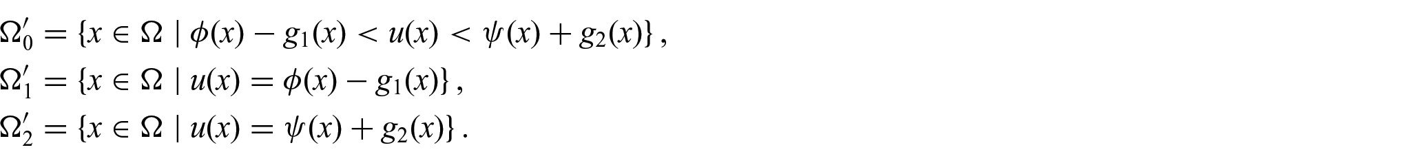
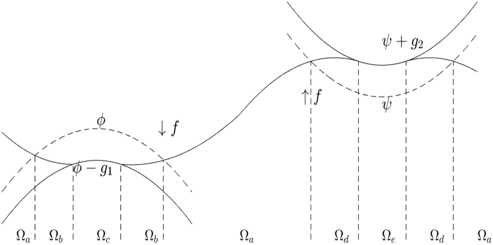
Now we obtain the equivalence of the energy form, the variational inequality form, and the differential equation form of this new bilateral obstacle problem. From (16), we can divide the domain $Ω$ into the following five parts:

\begin{matrix} ϕ < u < ψ and - Δ u = f in Ω_{a}, \\ ϕ - g_{1} < u < ϕ and - Δ u - p (ϕ - u) - f = 0 in Ω_{b}, \\ ψ < u < ψ + g_{2} and - Δ u + q (u - ψ) - f = 0 in Ω_{d}, \\ u = ϕ - g_{1} and - Δ u - c_{v} g_{1} - f \geq 0 in Ω_{c}, \\ u = ψ + g_{2} and - Δ u + d_{v} g_{2} - f \leq 0 in Ω_{e} . \end{matrix}

Note that $Ω_{a}$ indicates that there is no contact between the elastic membrane and the obstacles, $Ω_{b}$ and $Ω_{d}$ represent the overlapping part of elastic membrane and soft layers, and the elastic membrane does not completely penetrate the soft layers $g_{1}$ and $g_{2}$ . $Ω_{c}$ and $Ω_{e}$ represent the overlapping part of elastic membrane and rigid bodies. In Figure 1, a one-dimensional bilateral obstacle problem is visualized.

Figure 1.

One-dimensional bilateral obstacle problem.

Remark 1. The position of $Ω_{b}$ , $Ω_{c}$ , $Ω_{d}$ , and $Ω_{e}$ cannot be determined in advance. Therefore, the new bilateral obstacle problem is also a free boundary problem.

Remark 2. Obviously, when $g_{1}, g_{2} = 0$ , no interpenetration is allowed, this is a classical bilateral obstacle problem. When $g_{2} = 0$ , and $ψ$ takes infinity, this is a new kind of unilateral obstacle problem.

3. Numerical analysis

In this section, we first consider the finite element discretization numerical schemes for variational inequality (15), and derive the optimal order error estimate. Then, we apply the penalty method to approximate the constraint problem (17) and prove its convergence.

3.1. Optimal order error estimation of finite element approximation

Let us now describe the discretization of problem (15). Let $T_{h}$ be a “classical” triangulation [19] of $Ω$ with $h > 0$ denoting a spatial discretization parameter, and $N_{h}$ the set of nodes of $T_{h}$ . We approximate the following finite element space

V_{h} = {v_{h} \in C (\bar{Ω}), v_{h} |_{\partial Ω} = 0, v_{h} |_{T} \in P_{1}, \forall T \in T_{h}} \subset H_{0}^{1} (Ω),

where $P_{1}$ denotes the space of polynomials of degree at most one. Evidently, $V_{h}$ is a finite dimensional subspace of $H_{0}^{1} (Ω)$ , the admissible set $K$ has the following approximation:

K_{h} = {v_{h} \in V_{h} | (ϕ - g_{1}) (P) \leq v_{h} (P) \leq (ψ + g_{2}) (P), \forall P \in N_{h}} .

Hence, we immediately get the finite element approximation of variational inequality (15): Find $u_{h} \in K_{h}$ such that

a (u_{h}, v_{h} - u_{h}) + 〈 G u_{h}, v_{h} - u_{h} 〉 + 〈 F u_{h}, v_{h} - u_{h} 〉 \geq (f, v_{h} - u_{h}), \forall v_{h} \in K_{h} .

(17)

Here,

\begin{matrix} 〈 G u_{h}, v_{h} - u_{h} 〉 = - \int_{Ω} p (ϕ - u_{h}) (v_{h} - u_{h}) dx, \\ 〈 F u_{h}, v_{h} - u_{h} 〉 = \int_{Ω} q (u_{h} - ψ) (v_{h} - u_{h}) dx, \end{matrix}

where

p (ϕ - u_{h}) = {\begin{matrix} c_{v} {[ϕ - u_{h}]}_{+}, if ϕ - u_{h} < g_{1}, \\ c_{v} g_{1}, otherwise, \end{matrix}

and

q (u_{h} - ψ) = {\begin{matrix} d_{v} {[u_{h} - ψ]}_{+}, if u_{h} - ψ < g_{2}, \\ d_{v} g_{2}, otherwise . \end{matrix}

Now, we assume that $ϕ - g_{1}$ and $ψ + g_{2}$ are convex functions so that $K_{h} \subset K$ . And we consider the operator $A : H_{0}^{1} (Ω) \to H^{- 1} (Ω)$ defined by $A = - Δ + G + F$ . From the properties of $G$ and $F$ , it is obvious that $A$ is a strongly monotone Lipschitz continuous operator. By standard arguments (see, e.g. [22]), there exists a unique solution $u_{h} \in K_{h}$ to problem (17). The next we derive optimal order error estimate under the assumption of full regularity.

Theorem 4. Let $u$ and $u_{h}$ be the solutions of (15) and (17), respectively. Assuming $u \in H^{2} (Ω)$ , then

∥ u - u_{h} ∥_{H^{1} (Ω)} \leq ch

where the constant $c > 0$ depends on $u$ .

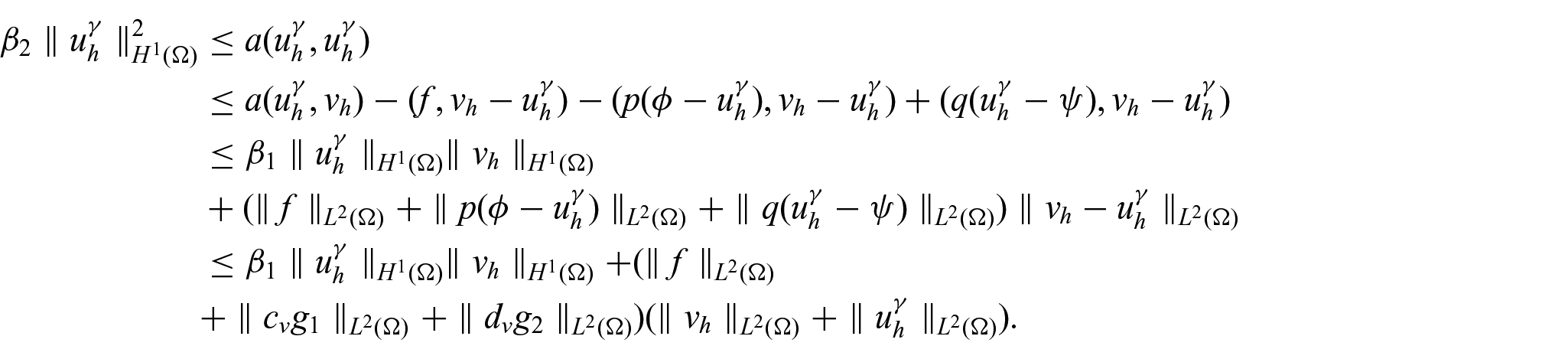
Proof. From the coercivity and bilinearity of $a$ , we have the following:

\begin{matrix} β_{2} ∥ u - u_{h} ∥_{H^{1} (Ω)}^{2} \leq a (u - u_{h}, u - u_{h}) \\ = a (u, u) + a (u_{h}, u_{h}) - a (u, u_{h}) - a (u_{h}, u) . \end{matrix}

(18)

Applying (15) and $K_{h} \subset K$ ,

a (u, u) \leq a (u, u_{h}) + 〈 Gu, u_{h} - u 〉 + 〈 Fu, u_{h} - u 〉 + (f, u - u_{h}) .

Let $v_{h} \in K_{h}$ be arbitrary. Then, according to (17), we obtain:

a (u_{h}, u_{h}) \leq a (u_{h}, v_{h}) + 〈 G u_{h}, v_{h} - u_{h} 〉 + 〈 F u_{h}, v_{h} - u_{h} 〉 + (f, u_{h} - v_{h}) .

Bringing the above two inequalities into (18), we obtain:

\begin{matrix} β_{2} ∥ u - u_{h} ∥_{H^{1} (Ω)}^{2} \leq a (u_{h}, v_{h} - u) + 〈 Gu, u_{h} - u 〉 + 〈 G u_{h}, v_{h} - u_{h} 〉 \\ + (Fu, u_{h} - u) + (F u_{h}, v_{h} - u_{h}) + (f, u - v_{h}) . \end{matrix}

(19)

By equations (8) and (9) and the monotonicity of $G$ , $F$ , we have the following:

\begin{matrix} 〈 Gu, u_{h} - u 〉 + 〈 G u_{h}, v_{h} - u_{h} 〉 = 〈 Gu - G u_{h}, u_{h} - u 〉 + 〈 G u_{h}, v_{h} - u 〉 \leq 〈 G u_{h}, v_{h} - u 〉, \\ 〈 Fu, u_{h} - u 〉 + 〈 F u_{h}, v_{h} - u_{h} 〉 = 〈 Fu - F u_{h}, u_{h} - u 〉 + 〈 F u_{h}, v_{h} - u 〉 \leq 〈 F u_{h}, v_{h} - u 〉 . \end{matrix}

Plugging this into (19) yields

\begin{matrix} β_{2} ∥ u - u_{h} ∥_{H^{1} (Ω)}^{2} \leq a (u_{h}, v_{h} - u) + 〈 G u_{h}, v_{h} - u 〉 + 〈 F u_{h}, v_{h} - u 〉 + (f, u - v_{h}) \\ = a (u_{h} - u, v_{h} - u) + R_{v_{h}}, \end{matrix}

(20)

where $R_{v_{h}} : = a (u, v_{h} - u) + 〈 G u_{h}, v_{h} - u 〉 + 〈 F u_{h}, v_{h} - u 〉 + (f, u - v_{h})$ . Now let us bound each term of (20). Since

a (u_{h} - u, v_{h} - u) \leq β_{1} ∥ u - u_{h} ∥_{H^{1} (Ω)} ∥ u - v_{h} ∥_{H^{1} (Ω)},

and

∥ u - u_{h} ∥_{H^{1} (Ω)} ∥ u - v_{h} ∥_{H^{1} (Ω)} \leq \frac{1}{2} (\frac{β_{2}}{β_{1}} ∥ u - u_{h} ∥_{H^{1} (Ω)}^{2} + \frac{β_{1}}{β_{2}} ∥ u - v_{h} ∥_{H^{1} (Ω)}^{2}) .

We obtain:

a (u_{h} - u, v_{h} - u) \leq \frac{β_{2}}{2} ∥ u - u_{h} ∥_{H^{1} (Ω)}^{2} + \frac{β_{1}^{2}}{2 β_{2}} ∥ u - v_{h} ∥_{H^{1} (Ω)}^{2} .

(21)

Since $u \in H^{2} (Ω)$ , we have the following:

a (u, v_{h} - u) = \int_{Ω} \nabla u \cdot \nabla (v_{h} - u) dx = - \int_{Ω} Δ u (v_{h} - u) dx \leq ∥ Δ u ∥_{L^{2} (Ω)} ∥ v_{h} - u ∥_{L^{2} (Ω)} .

Therefore,

\begin{matrix} R_{v_{h}} = a (u, v_{h} - u) + 〈 G u_{h}, v_{h} - u 〉 + 〈 F u_{h}, v_{h} - u 〉 + (f, u - v_{h}) \\ \leq (∥ Δ u ∥_{L^{2} (Ω)} + ∥ c_{v} g_{1} ∥_{L^{2} (Ω)} + ∥ d_{v} g_{2} ∥_{L^{2} (Ω)} + ∥ f ∥_{L^{2} (Ω)}) ∥ v_{h} - u ∥_{L^{2} (Ω)} . \end{matrix}

(22)

Combining the above results (21) and (22) with (20), we get that

\frac{β_{2}}{2} ∥ u - u_{h} ∥_{H^{1} (Ω)}^{2} \leq c inf_{v_{h} \in K_{h}} {∥ u - v_{h} ∥_{H^{1} (Ω)}^{2} + ∥ u - v_{h} ∥_{L^{2} (Ω)}} .

Hence, the Céa-type inequality is obtained as follows:

∥ u - u_{h} ∥_{H^{1} (Ω)} \leq c inf_{v_{h} \in K_{h}} {∥ u - v_{h} ∥_{H^{1} (Ω)} + ∥ u - v_{h} ∥_{L^{2} (Ω)}^{\frac{1}{2}}} .

Finally, applying standard finite element interpolation theory (see, e.g. [24]), under the assumption of $u \in H^{2} (Ω)$ , we obtain:

∥ u - u_{h} ∥_{H^{1} (Ω)} \leq ch .

□

3.2. Convergence results based on penalty method

For convenience, we let $\bar{ϕ} : = ϕ - g_{1}$ and $\bar{ψ} : = ψ + g_{2}$ . We use the penalty method to approximate the constraint problem (17) as follows: Find $u_{h}^{γ} \in V_{h}$ such that

a (u_{h}^{γ}, v_{h}) - (p (ϕ - u_{h}^{γ}), v_{h}) + (q (u_{h}^{γ} - ψ), v_{h}) + (r_{1} (γ; u_{h}^{γ}), v_{h}) + (r_{2} (γ; u_{h}^{γ}), v_{h}) = (f, v_{h}), \forall v_{h} \in V_{h},

(23)

where $γ > 0$ is a constant and we define $r_{1} (γ; u_{h}^{γ}) : = min {γ (u_{h}^{γ} - \bar{ϕ}), 0}$ , $r_{2} (γ; u_{h}^{γ}) : = \max {γ (u_{h}^{γ} - \bar{ψ}), 0}$ . From the definitions of $r_{1}$ and $r_{2}$ , it is easy to know that $r_{1}$ and $r_{2}$ are monotonic and Lipschitz continuous. Therefore, according to the Minty–Browder theorem [25], the solution of equation (23) exists and is unique for every $γ > 0$ . Furthermore, the following convergence theorem is obtained.

Theorem 5. The solution $u_{h}^{γ}$ of the penalty form (23) is uniformly bounded with respect to $γ$ , and when $γ \to \infty$ , the solution $u_{h}^{γ}$ converges to $u_{h}$ .

Proof. Take an element $v_{h}$ from $K_{h}$ , i.e. $\bar{ϕ} \leq v_{h} \leq \bar{ψ}$ . According to (23), we have

\begin{matrix} a (u_{h}^{γ}, v_{h} - u_{h}^{γ}) - (p (ϕ - u_{h}^{γ}), v_{h} - u_{h}^{γ}) + (q (u_{h}^{γ} - ψ), v_{h} - u_{h}^{γ}) \\ + (r_{1} (γ; u_{h}^{γ}), v_{h} - u_{h}^{γ}) + (r_{2} (γ; u_{h}^{γ}), v_{h} - u_{h}^{γ}) = (f, v_{h} - u_{h}^{γ}) . \end{matrix}

Since $r_{1} (γ; v_{h}) = 0$ and $r_{1}$ is monotonous, we obtain

(r_{1} (γ; u_{h}^{γ}), v_{h} - u_{h}^{γ}) = - (r_{1} (γ; v_{h}) - r_{1} (γ; u_{h}^{γ}), v_{h} - u_{h}^{γ}) \leq 0,

and since $r_{2} (γ; v_{h}) = 0$ , $r_{2}$ is monotonous, we have

(r_{2} (γ; u_{h}^{γ}), v_{h} - u_{h}^{γ}) = - (r_{2} (γ; v_{h}) - r_{2} (γ; u_{h}^{γ}), v_{h} - u_{h}^{γ}) \leq 0 .

Thus,

a (u_{h}^{γ}, v_{h} - u_{h}^{γ}) \geq (f, v_{h} - u_{h}^{γ}) + (p (ϕ - u_{h}^{γ}), v_{h} - u_{h}^{γ}) - (q (u_{h}^{γ} - ψ), v_{h} - u_{h}^{γ}), \forall v_{h} \in V_{h} .

(24)

Using the coercivity of $a$ , we get that

\begin{matrix} β_{2} ∥ u_{h}^{γ} ∥_{H^{1} (Ω)}^{2} \leq a (u_{h}^{γ}, u_{h}^{γ}) \\ \leq a (u_{h}^{γ}, v_{h}) - (f, v_{h} - u_{h}^{γ}) - (p (ϕ - u_{h}^{γ}), v_{h} - u_{h}^{γ}) + (q (u_{h}^{γ} - ψ), v_{h} - u_{h}^{γ}) \\ \leq β_{1} ∥ u_{h}^{γ} ∥_{H^{1} (Ω)} ∥ v_{h} ∥_{H^{1} (Ω)} \\ + (∥ f ∥_{L^{2} (Ω)} + ∥ p (ϕ - u_{h}^{γ}) ∥_{L^{2} (Ω)} + ∥ q (u_{h}^{γ} - ψ) ∥_{L^{2} (Ω)}) ∥ v_{h} - u_{h}^{γ} ∥_{L^{2} (Ω)} \\ \leq β_{1} ∥ u_{h}^{γ} ∥_{H^{1} (Ω)} ∥ v_{h} ∥_{H^{1} (Ω)} + (∥ f ∥_{L^{2} (Ω)} \\ + ∥ c_{v} g_{1} ∥_{L^{2} (Ω)} + ∥ d_{v} g_{2} ∥_{L^{2} (Ω)}) (∥ v_{h} ∥_{L^{2} (Ω)} + ∥ u_{h}^{γ} ∥_{L^{2} (Ω)}) . \end{matrix}

Therefore, $u_{h}^{γ}$ is uniformly bounded in $H_{0}^{1} (Ω)$ with respect to $γ$ .

In the finite dimensional space $V_{h}$ , there is a convergent subsequence ${u_{h}^{γ}}$ converging to some $w_{h} \in V_{h}$ . For the convenience of writing, we always denote that the subsequence is ${u_{h}^{γ}}$ . Let the limit $γ \to \infty$ in (24), we have the following:

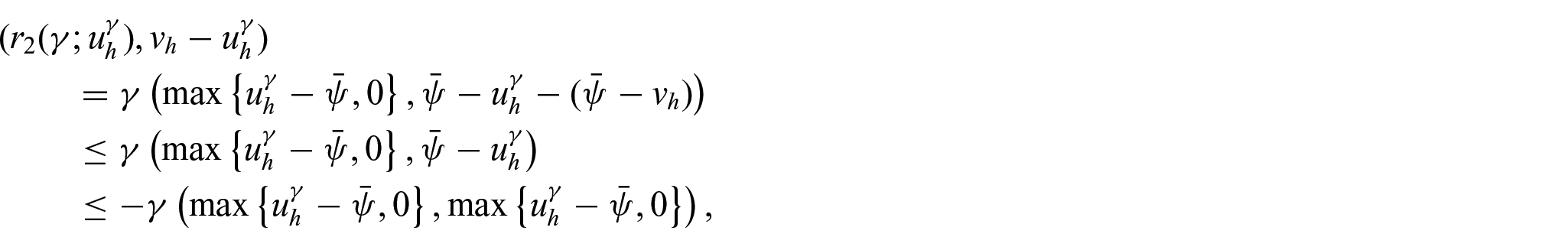
a (w_{h}, v_{h} - w_{h}) - (p (ϕ - w_{h}), v_{h} - w_{h}) + (q (w_{h} - ψ), v_{h} - w_{h}) \geq (f, v_{h} - w_{h}), \forall v_{h} \in V_{h} .

Now, we are in the position to show $w_{h} \in K_{h}$ . Let $w_{h} \in V_{h}$ and put $v_{h} - u_{h}^{γ}$ instead of $v_{h}$ in (23), we obtain:

\begin{matrix} a (u_{h}^{γ}, v_{h} - u_{h}^{γ}) - (p (ϕ - u_{h}^{γ}), v_{h} - u_{h}^{γ}) + (q (u_{h}^{γ} - ψ), v_{h} - u_{h}^{γ}) \\ + (r_{1} (γ; u_{h}^{γ}), v_{h} - u_{h}^{γ}) + (r_{2} (γ; u_{h}^{γ}), v_{h} - u_{h}^{γ}) = (f, v_{h} - u_{h}^{γ}) . \end{matrix}

Since

\begin{matrix} (r_{1} (γ; u_{h}^{γ}), v_{h} - u_{h}^{γ}) \\ = γ (\min {u_{h}^{γ} - \bar{ϕ}, 0}, v_{h} - \bar{ϕ} - (u_{h}^{γ} - \bar{ϕ})) \\ \leq - γ (\min {u_{h}^{γ} - \bar{ϕ}, 0}, u_{h}^{γ} - \bar{ϕ}) \\ \leq - γ (\min {u_{h}^{γ} - \bar{ϕ}, 0}, \min {u_{h}^{γ} - \bar{ϕ}, 0}), \end{matrix}

and

\begin{matrix} (r_{2} (γ; u_{h}^{γ}), v_{h} - u_{h}^{γ}) \\ = γ (\max {u_{h}^{γ} - \bar{ψ}, 0}, \bar{ψ} - u_{h}^{γ} - (\bar{ψ} - v_{h})) \\ \leq γ (\max {u_{h}^{γ} - \bar{ψ}, 0}, \bar{ψ} - u_{h}^{γ}) \\ \leq - γ (\max {u_{h}^{γ} - \bar{ψ}, 0}, \max {u_{h}^{γ} - \bar{ψ}, 0}), \end{matrix}

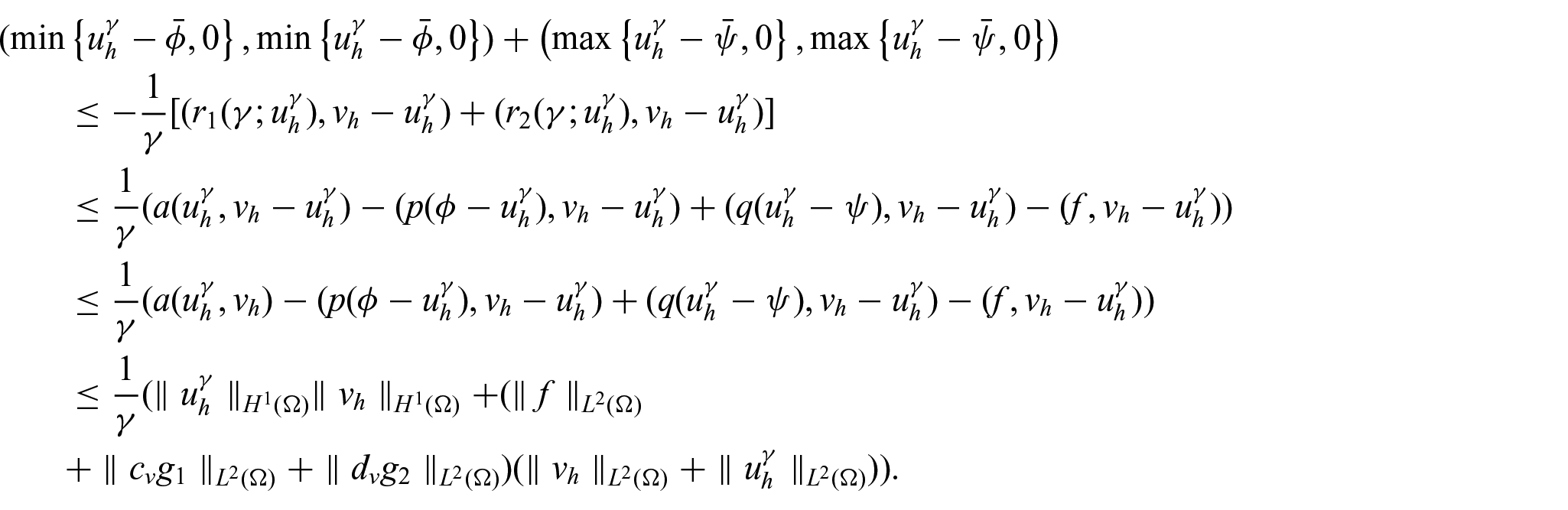
we obtain

\begin{matrix} (\min {u_{h}^{γ} - \bar{ϕ}, 0}, \min {u_{h}^{γ} - \bar{ϕ}, 0}) + (\max {u_{h}^{γ} - \bar{ψ}, 0}, \max {u_{h}^{γ} - \bar{ψ}, 0}) \\ \leq - \frac{1}{γ} [(r_{1} (γ; u_{h}^{γ}), v_{h} - u_{h}^{γ}) + (r_{2} (γ; u_{h}^{γ}), v_{h} - u_{h}^{γ})] \\ \leq \frac{1}{γ} (a (u_{h}^{γ}, v_{h} - u_{h}^{γ}) - (p (ϕ - u_{h}^{γ}), v_{h} - u_{h}^{γ}) + (q (u_{h}^{γ} - ψ), v_{h} - u_{h}^{γ}) - (f, v_{h} - u_{h}^{γ})) \\ \leq \frac{1}{γ} (a (u_{h}^{γ}, v_{h}) - (p (ϕ - u_{h}^{γ}), v_{h} - u_{h}^{γ}) + (q (u_{h}^{γ} - ψ), v_{h} - u_{h}^{γ}) - (f, v_{h} - u_{h}^{γ})) \\ \leq \frac{1}{γ} (∥ u_{h}^{γ} ∥_{H^{1} (Ω)} ∥ v_{h} ∥_{H^{1} (Ω)} + (∥ f ∥_{L^{2} (Ω)} \\ + ∥ c_{v} g_{1} ∥_{L^{2} (Ω)} + ∥ d_{v} g_{2} ∥_{L^{2} (Ω)}) (∥ v_{h} ∥_{L^{2} (Ω)} + ∥ u_{h}^{γ} ∥_{L^{2} (Ω)})) . \end{matrix}

By the boundedness of $u_{h}^{γ}$ , we have

(\min {u_{h}^{γ} - \bar{ϕ}, 0}, \min {u_{h}^{γ} - \bar{ϕ}, 0}) + (\max {u_{h}^{γ} - \bar{ψ}, 0}, \max {u_{h}^{γ} - \bar{ψ}, 0}) \leq \frac{c}{γ} .

let $γ \to \infty$ , we obtain

(\min {u_{h}^{γ} - \bar{ϕ}, 0}, \min {u_{h}^{γ} - \bar{ϕ}, 0}) = 0,

and

(\max {u_{h}^{γ} - \bar{ψ}, 0}, \max {u_{h}^{γ} - \bar{ψ}, 0}) = 0 .

Then, we deduce that

\min {w_{h} - \bar{ϕ}, 0} = 0 a . e . in Ω,

and

\max {w_{h} - \bar{ψ}, 0} = 0 a . e . in Ω .

That is, $w_{h} \in K_{h}$ . Therefore, the limit $w_{h} = u_{h}$ is the unique solution of problem (17), i.e. the solution $u_{h}^{γ}$ converges to $u_{h}$ as $γ \to \infty$ . □

4. Numerical results

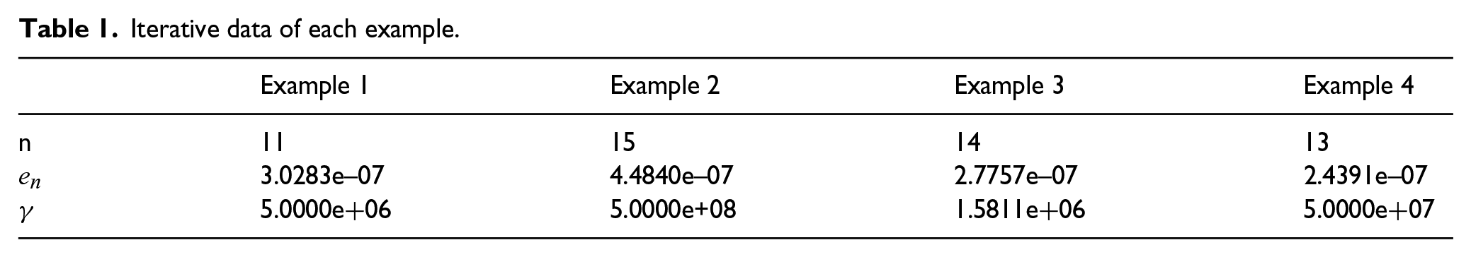
We use four numerical examples to support the previous theoretical analysis. All experiments are performed on an Intel Dual-Core personal computer with Matlab version R2019a. For convenience, in all the following examples, we take $Ω = [0, 1] \times [0, 1]$ and $c_{v} = d_{v} = 1$ , the absolute error $e_{n + 1} = ∥ u^{n + 1} - u^{n} ∥_{L^{2} (Ω)} \leq ε_{0} = 10^{- 6}$ as the stop criterion, and $n$ as the number of iterations. Without lose of generality, we take the initial penalty parameter $γ_{0} = 50$ and keep updating $γ_{n + 1} \leftarrow \sqrt{10} γ_{n}$ as the iteration progresses, and we consider that the mesh size is $\frac{1}{64}$ .

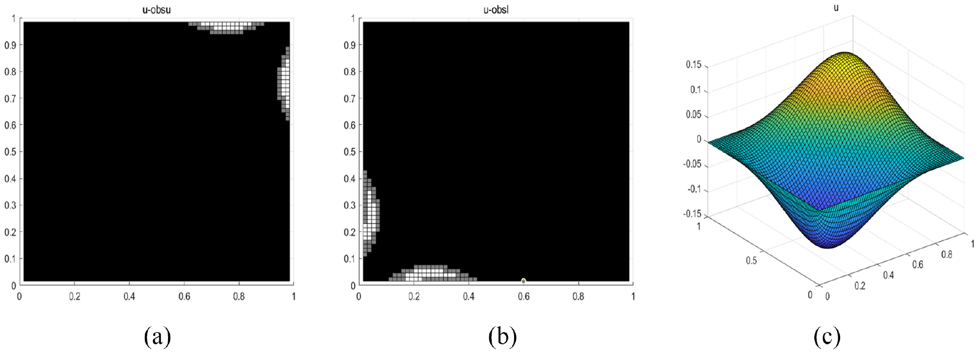
Example 1. We consider this example from the works by Ran and Cheng [1], Murea and Tiba [11], and Cheng et al. [18]. Here, $ϕ (x, y) = - dist ((x, y), \partial Ω)$ , $ψ (x, y) = dist ((x, y), \partial Ω)$ , $f (x, y) = 11 (x + y - 1)$ , and let $g_{1} (x, y) = 0.001, g_{2} (x, y) = 0.001$ . Then, we get the numerical results and iterative data as shown in Figure 2 and Table 1, respectively.

Figure 2.

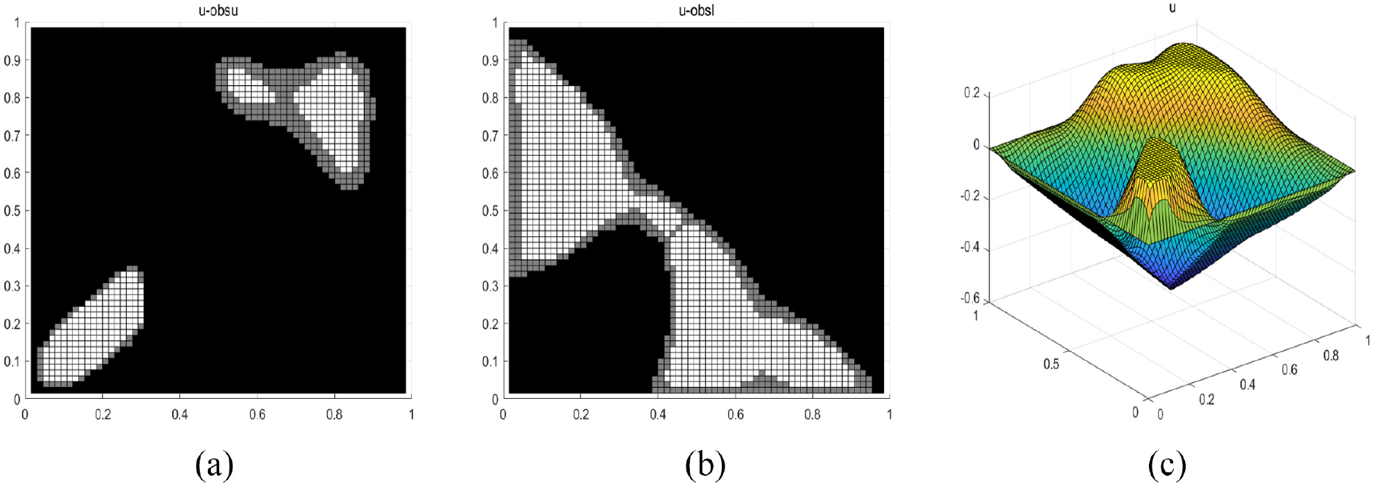
Numerical results of example 1: (a) the upper contact sets, (b) the lower contact sets, and (c) the numerical solution.

Table 1.

Iterative data of each example.

	Example 1	Example 2	Example 3	Example 4
n	11	15	14	13
$e_{n}$	3.0283e–07	4.4840e–07	2.7757e–07	2.4391e–07
$γ$	5.0000e +06	5.0000e+08	1.5811e +06	5.0000e +07

Example 2. We consider a two-dimensional bilateral obstacle problem, which had been reported in the works by Ran and Cheng [1], Kärkkäinen [7] and Cheng et al. [18], i.e. $ϕ (x, y) = - dist ((x, y), \partial Ω), ψ (x, y) = 0.2$ , set $g_{1} (x, y) = 0.01, g_{2} (x, y) = 0.01$ and

f (x, y) = {\begin{matrix} 300, & if (x, y) \in S = (x, y) \in Ω : | x - y | \leq 0.1 and x \leq 0.3, \\ - 70 e^{y} g (x), & if x \leq 1 - y and (x, y) \notin S, \\ 15 e^{y} g (x), & if x > 1 - y and (x, y) \notin S . \end{matrix}

where

g (x) = {\begin{matrix} 6 x, & if 0 < x \leq \frac{1}{6}, \\ 2 (1 - 3 x), & if \frac{1}{6} < x \leq \frac{1}{3}, \\ 6 (x - \frac{1}{3}), & if \frac{1}{3} < x \leq \frac{1}{2}, \\ 2 (1 - 3 (x - \frac{1}{3})), & if \frac{1}{2} < x \leq \frac{2}{3}, \\ 6 (x - \frac{2}{3}), & if \frac{2}{3} < x \leq \frac{5}{6}, \\ 2 (1 - 3 (x - \frac{2}{3})), & if \frac{5}{6} < x \leq 1 . \end{matrix}

The corresponding numerical results are clearly seen in Figure 3 and Table 1.

Figure 3.

Numerical results of example 2: (a) the upper contact sets, (b) the lower contact sets, and (c) the numerical solution.

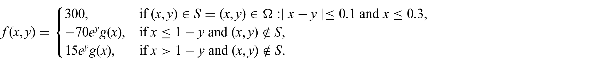
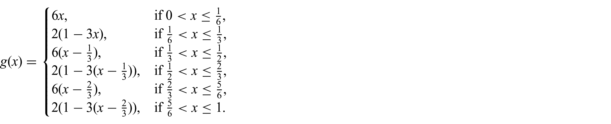
Example 3. The load and obstacle function are $f = - 20$ and $ϕ (x, y) = 10 x (1 - x) y (1 - y) - \frac{1}{2}$ from the works by Imoro [6] and Cheng et al. [18]; set $ψ (x, y) = 0.2$ , $g_{1} (x, y) = 0.01$ , and $g_{2} (x, y) = 0.01$ . The corresponding results are shown in Figure 4 and Table 1, respectively.

Figure 4.

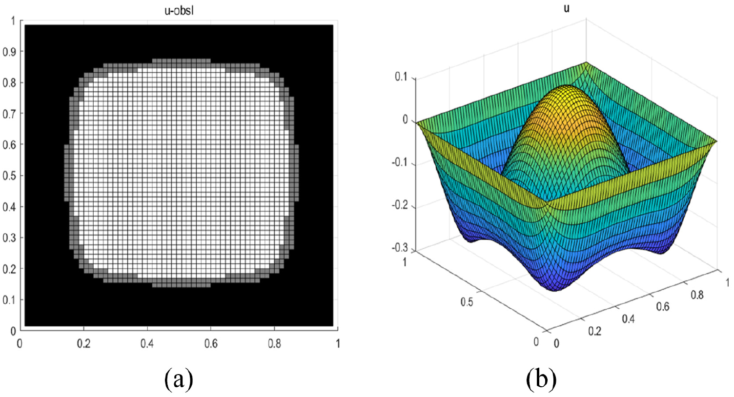
Numerical results of example 3: (a) the lower contact sets and (b) the numerical solution.

Example 4. Let the obstacle function $f = 45 (x - x^{2}) (\sin (11 π x) + 1)$ , and $ϕ (x, y) = - \infty, ψ (x, y) = dist ((x, y), \partial Ω)$ from the works by Ran and Cheng [1] and Kärkkäinen [7]; set $g_{1} (x, y) = 0.001$ , $g_{2} (x, y) = 0.001$ . We show the corresponding numerical results in Figure 5 and Table 1.

Figure 5.

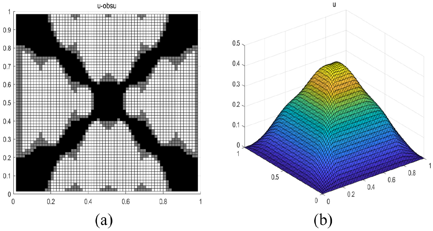
Numerical results of example 4: (a) the upper contact sets and (b) the numerical solution.

The numerical results of the above examples are shown in Figures 2 –5. In the contact sets, the coincidence part between the elastic membrane and the soft layers are marked in gray, the coincidence region of the elastic membrane and the rigid bodies are marked in white, and black part represents non-coincidence region of the elastic membrane. It should be noted that the elastic membrane in example 3 did not contact the upper obstacle, and the elastic membrane in example 4 did not contact the lower obstacle.

5. Conclusion

In this paper, we studied a new kind of elastic-rigid bilateral obstacle problem. Under certain assumptions, we obtain three forms to describe the problem and prove their equivalence. Based on the variational inequality form, we derived the optimal order error estimate. Moreover, the numerical results showed that the simulation results are in line with the theoretical analysis.

Footnotes

Acknowledgements

The authors would like to thank the anonymous reviewers for their valuable comments and suggestions.

Funding

The author(s) disclosed receipt of the following financial support for the research, authorship, and/or publication of this article: This work was supported by scientific research project of introducing talents of Guizhou University (no. X2022103).

ORCID iD

Qinghua Ran

References

Ran

Cheng

A new numerical method for solving a bilateral obstacle problem. Appl Math J Chinese Univ Ser A 2021; 36(2): 208–216.

Bouchlaghem

Mermri

Analysis of a mixed formulation of a bilateral obstacle problem. Appl Math Comput 2018; 320: 45–55.

Bouchlaghem

Mermri

A Uzawa algorithm with multigrid solver for a bilateral obstacle problem. Appl Math Comput 2021; 389: 125553.

Duvaut

Lions

Inequalities in mechanics and physics (grundlehren der mathematischen wissenschaften). Berlin: Springer, 1976.

Hoppe

Multigrid algorithms for variational inequalities. SIAM J Numer Anal 1987; 24(5): 1046–1065.

Imoro

Discretized obstacle problems with penalties on nested grids. Appl Numer Math 2000; 32(1): 21–34.

Kärkkäinen

Kunisch

Tarvainen

Augmented Lagrangian active set methods for obstacle problems. J Optim Theory Appl 2003; 119(3): 499–533.

Kinderlehrer

Stampacchia

An introduction to variational inequalities and their applications (classics in applied mathematics, society for industrial and applied mathematics). Philadelphia, PA: SIAM, 2000.

Kornhuber

Monotone multigrid methods for elliptic variational inequalities I. Numer Math 1994; 69(2): 167–184.

10.

Kornhuber

Monotone multigrid methods for elliptic variational inequalities II. Numer Math 1996; 72(4): 481–499.

11.

Murea

Tiba

A penalization method for the elliptic bilateral obstacle problem. IFIP Adv Inform Commun Tech 2014; 443: 189–98.

12.

Murea

Tiba

A direct algorithm in some free boundary problems. J Numer Math 2016; 24(4): 253–271.

13.

Ran

Cheng

Abide

A dynamical method for solving the obstacle problem. Numer Math Theory Methods Appl 2020; 13(2): 353–371.

14.

Rodrigues

Obstacle problems in mathematical physics (North-Holland mathematics studies). Amsterdam: North-Holland Publishing, 1987.

15.

Tarvainen

Numerical algorithms based on characteristic domain decomposition for obstacle problems. Comm Numer Methods Eng 1997; 13(10): 793–801.

16.

Yuan

Cheng

An iterative algorithm based on the piecewise linear system for solving bilateral obstacle problems. Int J Comput Math 2012; 89(17): 2374–2384.

17.

Han

Sofonea

Convergence analysis of penalty based numerical methods for constrained inequality problems. Numer Math 2019; 142(4): 917–940.

18.

Cheng

Ran

Wang

, et al. Numerical analysis for a new kind of obstacle problem. Commun Nonlinear Sci Numer Simulat 2021; 99: 105810.

19.

Glowinski

Numerical methods for nonlinear variational problems (Springer series in computational physics, package array warning: redefining primitive column l on input line 670). Berlin: Springer, 1984.

20.

Klarbring

Mikelić

Shillor

On friction problems with normal compliance. Nonlinear Anal 1989; 13(8): 935–955.

21.

Rochdi

Shillor

Sofonea

Quasistatic viscoelastic contact with normal compliance and friction. J Elasticity 1998; 51(2): 105–126.

22.

Sofonea

Matei

Mathematical models in contact mechanics. Cambridge: Cambridge University Press, 2012.

23.

Ciarlet

PG.

Linear and nonlinear functional analysis with applications. Philadelphia, PA: Society for Industrial and Applied Mathematics, 2013.

24.

Brenner

Scott

The mathematical theory of finite element methods (texts in applied mathematics). Berlin: Springer, 2008.

25.

Carlos

Reyes

Numerical PDE-constrained optimization (SpringerBriefs in optimization). Berlin: Springer, 2015.