
Abstract
In this study, a peridynamic formulation is proposed for analysis of planar arbitrarily curved beams. Assumptions of Timoshenko–Ehrenfest beam model are considered such that linear kinematic relations are described by displacements of the beam axis and rotation of the cross-section. Equilibrium conditions and boundary conditions are derived by means of the principle of virtual work. Then, peridynamic functions are constructed, and incorporated with equilibrium conditions to develop a peridynamic formulation. Several examples are exhibited to examine the performance of the proposed formulation in some regards, i.e., numerical accuracy, convergence properties, and locking effects. It is delineated that the proposed formulation provides a good level of precision for the analysis of relatively thick beams. However, membrane and shear locking effects are present in the analysis of slender beams, and peridynamic functions of higher polynomial degree can be used to mitigate these unfavorable effects.
Keywords
1. Introduction
In classical continuum mechanics, equations of motion are written as partial differential equations, which are not well-defined with the presence of discontinuities. Consequently, peridynamic theory [1–5] has been introduced as a reformulation of classical continuum mechanics to eliminate their roadblocks in simulation of damage of solid bodies. Indeed, equations of motion in the peridynamic theory are expressed as integro-differential equations, which are valid on discontinuities. Furthermore, the peridynamic theory can be classified as a nonlocal one, meaning that a material particle interacts with other counterparts within a finite distance. These two distinct features make the peridynamic theory suitable for solving problems with evolving discontinuities and significant nonlocality [6–15].
In the implementation of the peridynamic theory, each material particle requires the construction of its own equations of motion, which involves its own unknown variables as well as those of other particles it interacts with. Consequently, the obtained system of equations is normally large and non-symmetric, and computational costs of the peridynamic theory become prohibitively expensive for the analysis of three-dimensional objects. Indeed, for the analysis of slender structures such as beams or plates, several layouts of particles along the direction of thickness are essential to ensure precise analysis [16] if these structures are simulated as fully three-dimensional objects. In this scenario, it is beneficial to develop formulations by incorporating dimension-reduced structural models with the peridynamic theory for the simulation of slender three-dimensional objects.
Regarding beam models, Timoshenko–Ehrenfest considers shear deformation by decoupling the deformation mechanisms of the beam axis and the cross-section. More precisely, the rigid cross-section is not necessarily always orthogonal to the beam axis during deformation. Hence, the Timoshenko–Ehrenfest beam model is widely used since it is capable of simulating both thick and thin beams. Recently, several beam formulations [17–26] have been developed in the context of peridynamic theory using kinematic assumptions of Timoshenko–Ehrenfest beam model. The common approach to derive the peridynamic equations of motion is first to construct the nonlocal expressions of the kinetic and total potential energy, and then use the Euler–Lagrange equation to obtain the equations of motion for each particle. This approach has been performed in previous works [17,18,21,24,25] for the geometrically linear analysis and in Nguyen and Oterkus [22] for the geometrically nonlinear analysis. The incorporation of peridynamic beam formulations with the finite element framework is carried out by Jafari et al. [19] and Yang et al. [20]. An alternative approach is to use the existing governing equations derived from the classical continuum mechanics with peridynamic differential operator [26], which converts the local derivatives into the nonlocal integration.
It is well known that the numerical precision of Timoshenko–Ehrenfest beam formulations can be degraded in analysis of slender beams owing to membrane and shear locking effects. These unfavorable effects have been observed with some other numerical methods, e.g., finite element methods [27–29], isogeometric analysis [30–36], and mesh-free methods [37]. For Timoshenko–Ehrenfest beam formulations with peridynamic theory, the presence of membrane and shear locking effects is also confirmed [24,25].
With the publications reviewed above, it is recognized that a locking-free peridynamic Timoshenko–Ehrenfest beam formulation for analysis of beams having arbitrary geometry has not yet been introduced. In this study, a peridynamic Timoshenko–Ehrenfest beam formulation is presented for the analysis of planar arbitrarily curved beams, and locking effects on numerical performance of the proposed formulation are examined. More precisely, with assumptions of Timoshenko–Ehrenfest beam model, displacements of the beam axis and the rotation of cross-section are used to describe linear kinematic relations. Equilibrium conditions together with boundary conditions are derived by means of the principle of virtual work. Then, a peridynamic formulation is developed by incorporating peridynamic functions with derived equilibrium conditions.
The rest of this paper is structured as follows. Section 2 involves the derivation of equilibrium conditions and boundary conditions of planar arbitrarily curved beams using kinematic assumptions of Timoshenko–Ehrenfest beam model. Section 3 presents the detailed construction of peridynamic functions using the concept of peridynamic differential operators [38,39], and the proposed peridynamic formulation is detailed. In section 4, three examples with several rigorous tests are designed to elucidate the performance of the proposed formulation. Conclusions are given in section 5.
2. Equilibrium conditions and boundary conditions of planar curved beams with Timoshenko–Ehrenfest beam model
In this section, linear kinematic relations of planar curved beams obeying assumptions of Timoshenko–Ehrenfest beam model are briefly detailed. Then, generalized strain and stress measures are presented for use of the principle of virtual work to derive equilibrium conditions and boundary conditions of planar arbitrarily curved beams.
2.1. Linear kinematic relations
A representative planar curved beam is pictorially portrayed in Figure 1. In the following derivations, the beam axis is assumed to be a regular curve, and parameterized by the arc length parameter
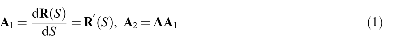
where
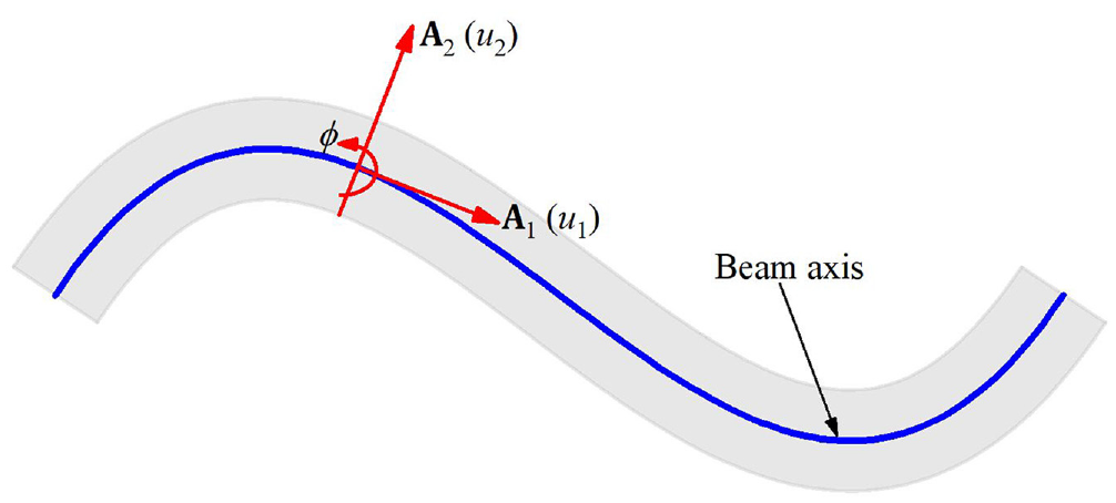
A representative planar arbitrarily curved beam.
In the context of Timoshenko–Ehrenfest beam model, the rigid cross-section does not necessarily remain orthogonal to the beam axis during deformation. Hence, linear kinematic relations of planar curved beams are described by the displacement vector

where
The deformation state of the beam is characterized by the membrane strain

with
In this study, only linear elastic isotropic materials are considered, and consequently, the following constitutive relations are used as below:

where
2.2. Equilibrium conditions and boundary conditions
For planar curved beams, the internal virtual work
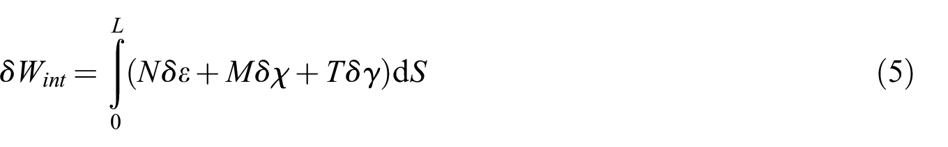
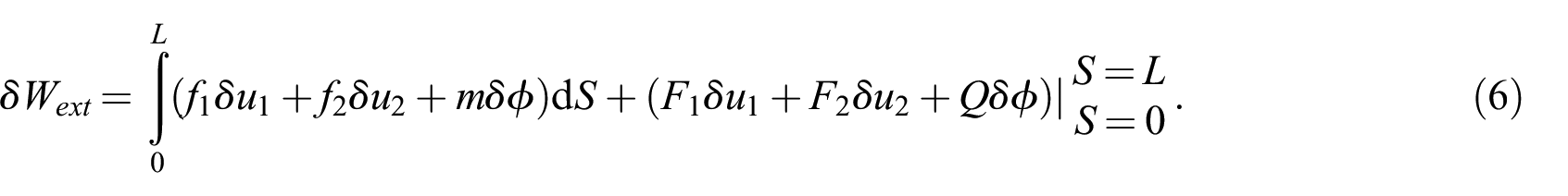
Here,
The principle of virtual work is now expressed as follows:

With the aid of Equations (3)–(7), one can arrive at the equilibrium conditions together with boundary conditions by employing the integration by parts and fundamental theorem of variational calculus, as follows.
Equilibrium conditions:


Boundary conditions:


The overlines signify prescribed values of the displacement components and cross-sectional rotation at the boundary.
The primal forms of the equilibrium conditions and boundary conditions are obtained by substituting Equations (3) and (4) into Equations (8)–(13) as below.
Primal forms of the equilibrium conditions:


Primal forms of the boundary conditions:


3. Peridynamic formulation for planar arbitrarily curved beams
This section discusses the construction of univariate peridynamic functions. Then, a peridynamic formulation for the analysis of planar curved beams is derived by means of the peridynamic functions.
3.1. Discretization and numerical integration scheme
Prior to detailed construction of the peridynamic functions, a quadrature scheme for numerical integration is discussed. Figure 2 exhibits a specific discretization of a beam axis with
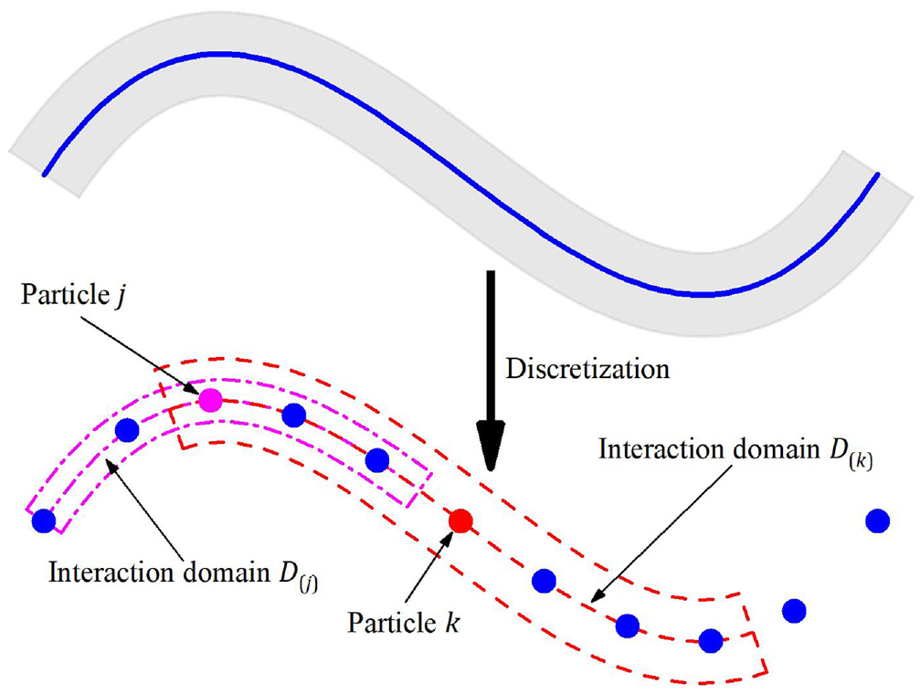
A peridynamic discretization.
A particle

where
Given a scalar-valued function
It is worth noting that the quadrature scheme mentioned above is not limited to uniform distributions of material particles. In practice, it is beneficial to employ discretization with nonuniform distributions of material particles for the analysis of beams having arbitrary geometry. Furthermore, the horizon is not necessarily a constant quantity, meaning that different values of horizon can be assigned to different particles. As illustrated in Figure 2, the particles
3.2. Peridynamic functions
In the vicinity of a material particle
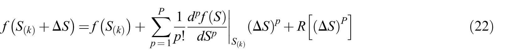
where
At particle
with
With the aid of Taylor series expansion and peridynamic functions, the derivatives of any order can be evaluated at particle
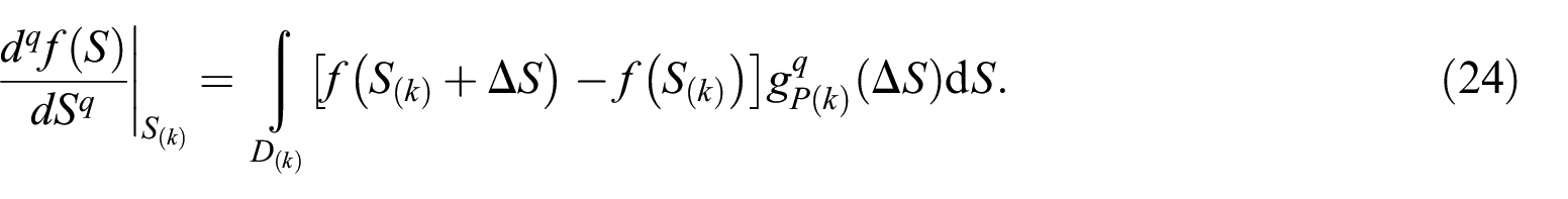
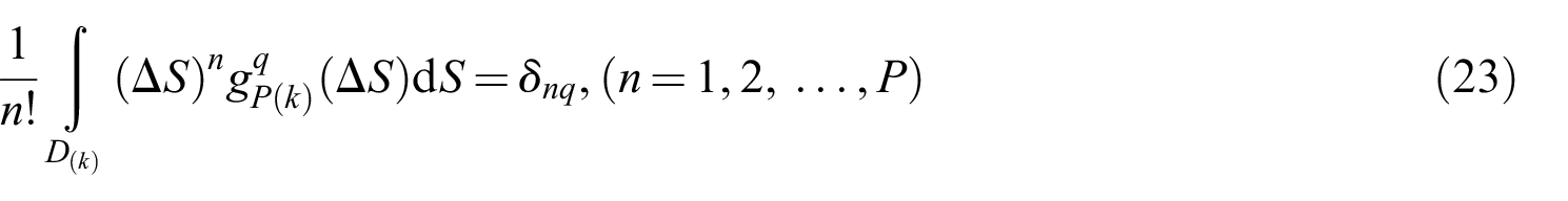
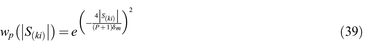
The remaining issue is the explicit forms of peridynamic functions. Although not a limitation, the peridynamic functions are commonly constructed as polynomials, i.e.,
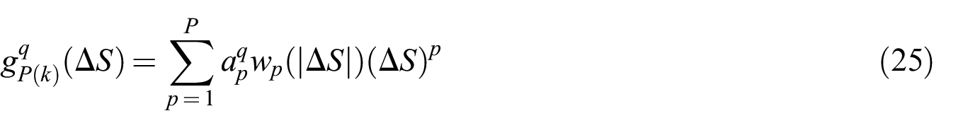
where
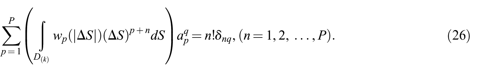
The determination of the unknown coefficients
3.3. Peridynamic formulation for planar curved beams
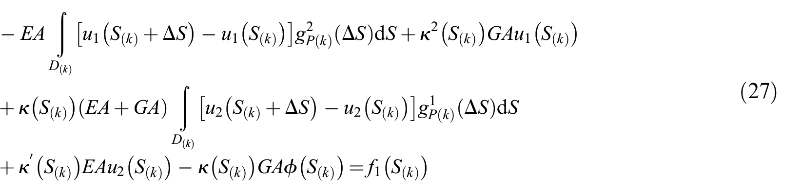
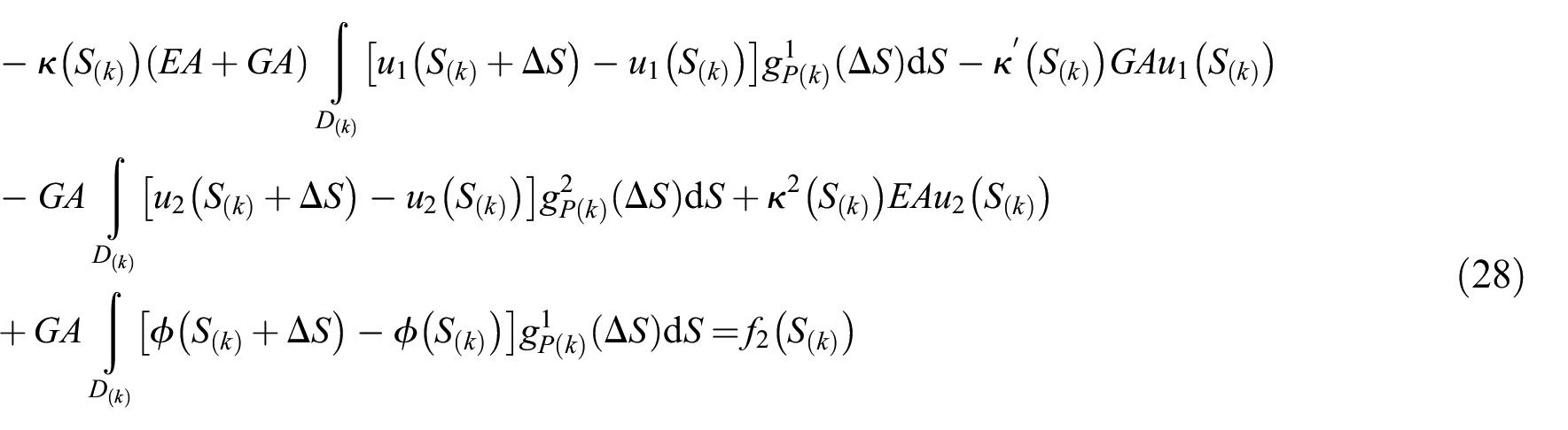
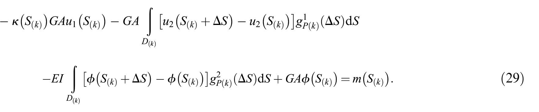
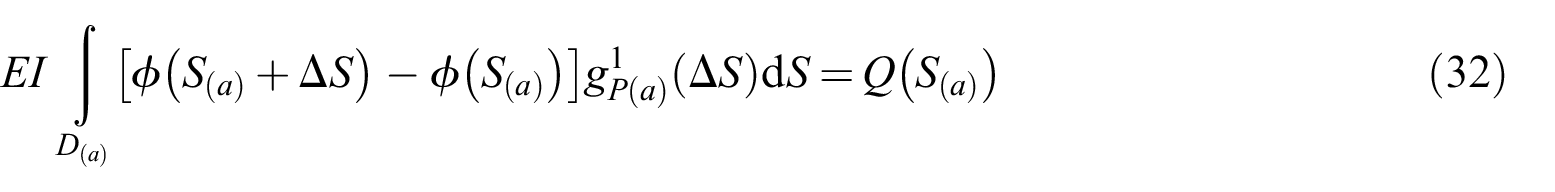
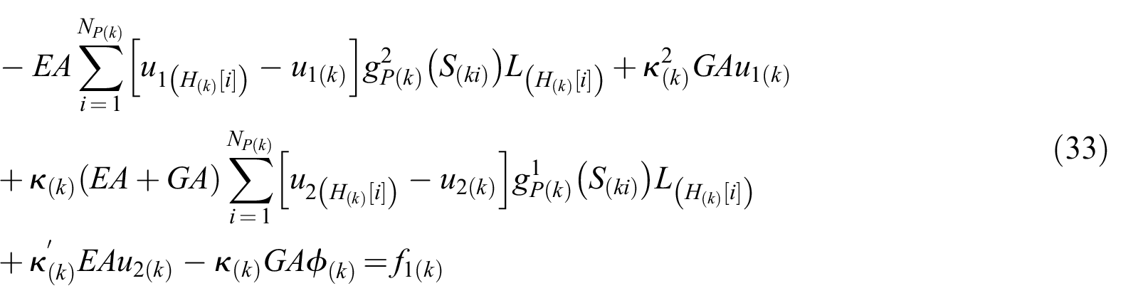
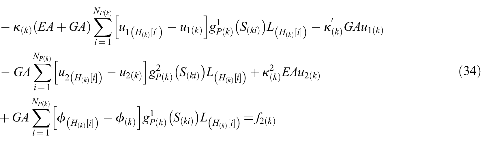
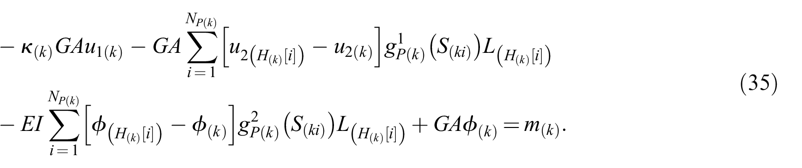
By incorporating the peridynamic functions into Equations (14)–(16), the equilibrium conditions of a particle
Furthermore, in case the loads are prescribed, the boundary conditions in Equation (17)–(19) can be alternatively written as follows:
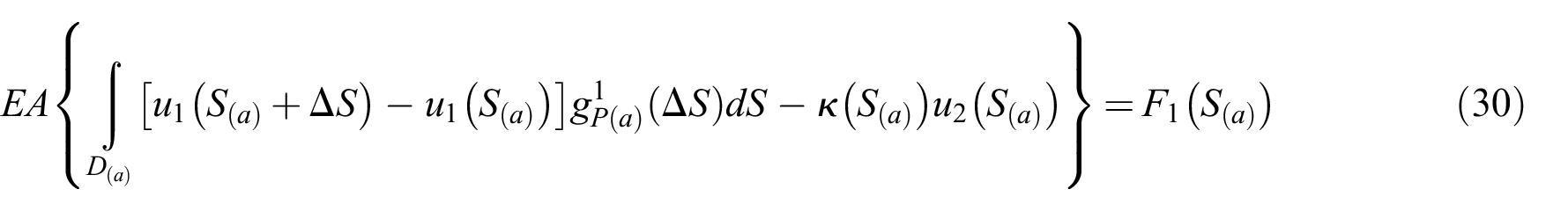
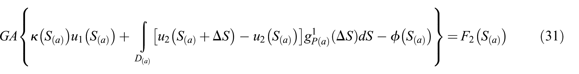
with
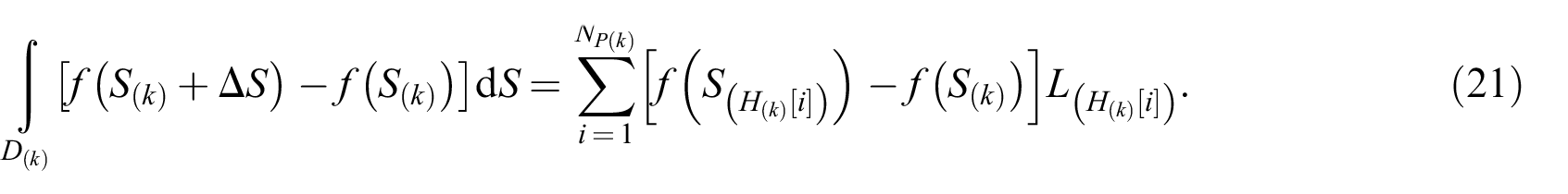
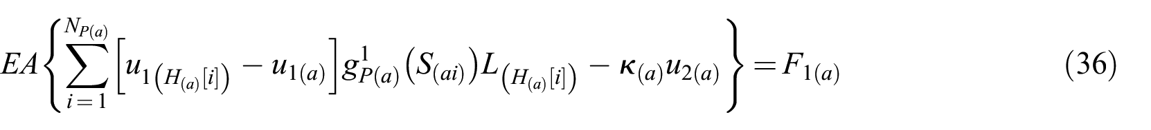
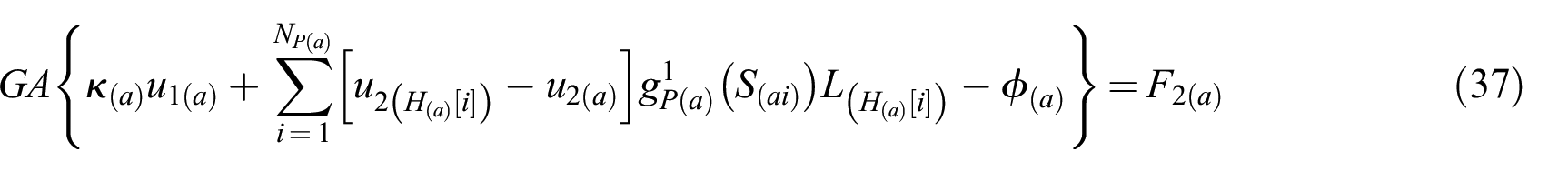
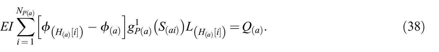
For numerical implementation, the integration involved in Equations (27)–(32) is performed by means of quadrature scheme presented in section 3.1. Consequently, the equilibrium conditions at particle
Here,
In an analogous fashion, the boundary conditions in Equations (30)–(32) are alternatively expressed as follows:
4. Illustrative examples
This section presents three examples to assess the performance of the proposed peridynamic formulation for the analysis of planar arbitrarily curved beams. Some remarks regarding numerical implementation are given before detailed discussions. In all tests, Young’s modulus
where
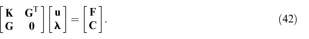
The enforcement of the equilibrium conditions at all particles leads to a system of linear equations as follows:

in which

where
Here,
Regarding cross-sectional geometry, square cross-sections with the side length of
4.1. A straight beam subjected to sinusoidal force
The first example deals with the analysis of a straight beam. As visualized in Figure 3, a straight beam is fixed at both ends, and subjected to a sinusoidal force described as follows:
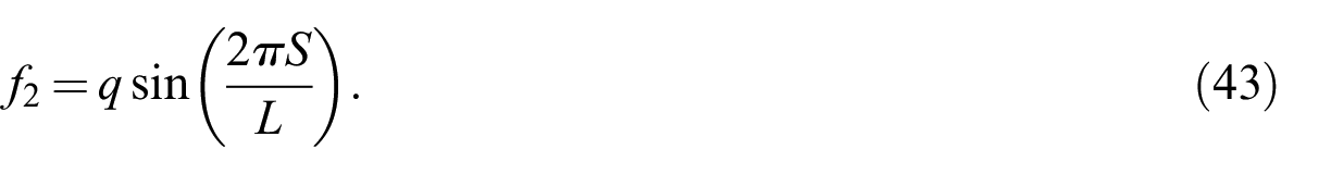
with


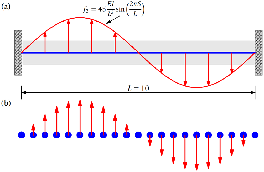
A straight beam subjected to sinusoidal force. (a) Problem setup. (b) A peridynamic discretization.
In this example, discretization with uniform distributions of material particles is employed. In the first test, the side length of the cross-section is set as
A straight beam subjected to sinusoidal force—numerical results with
The convergence properties of the proposed formulation are investigated with respect to different values of
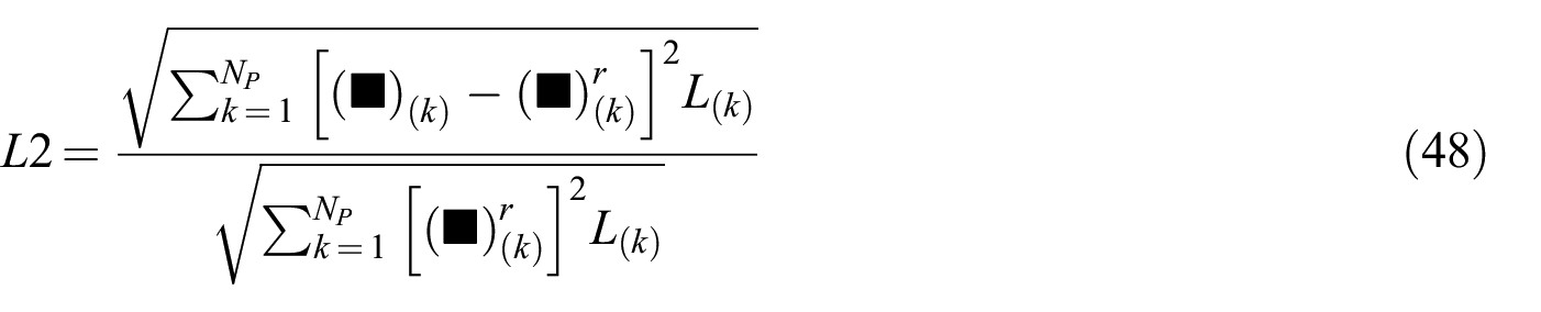
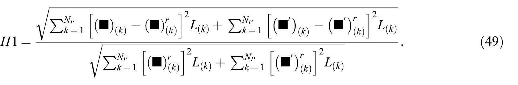
Here,
In the convergence tests, the relative errors are considered as the functions of the number of particles
A straight beam subjected to sinusoidal force—convergence results with
To scrutinize the shear locking effect on the numerical performance of the proposed formulation, the convergence tests are performed with
A straight beam subjected to sinusoidal force—convergence results with
4.2. A semi-circular beam
The second example is devoted to the analysis of a semi-circular beam of radius
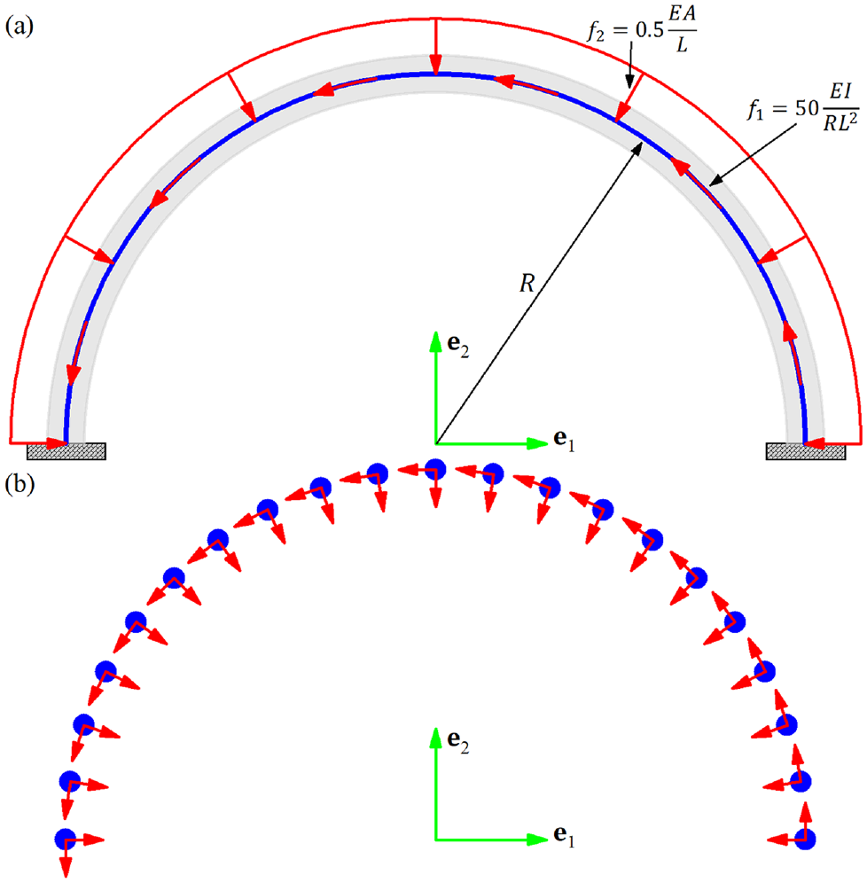
A semi-circular beam. (a) Problem setup. (b) A peridynamic discretization.
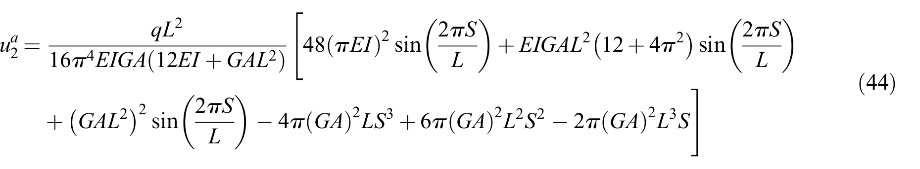
Discretization with uniform distributions of material particles is used for all tests of this example. The analytical solutions can be attained with the procedure detailed in the Appendix.
The slenderness of the semi-circular beam is defined as
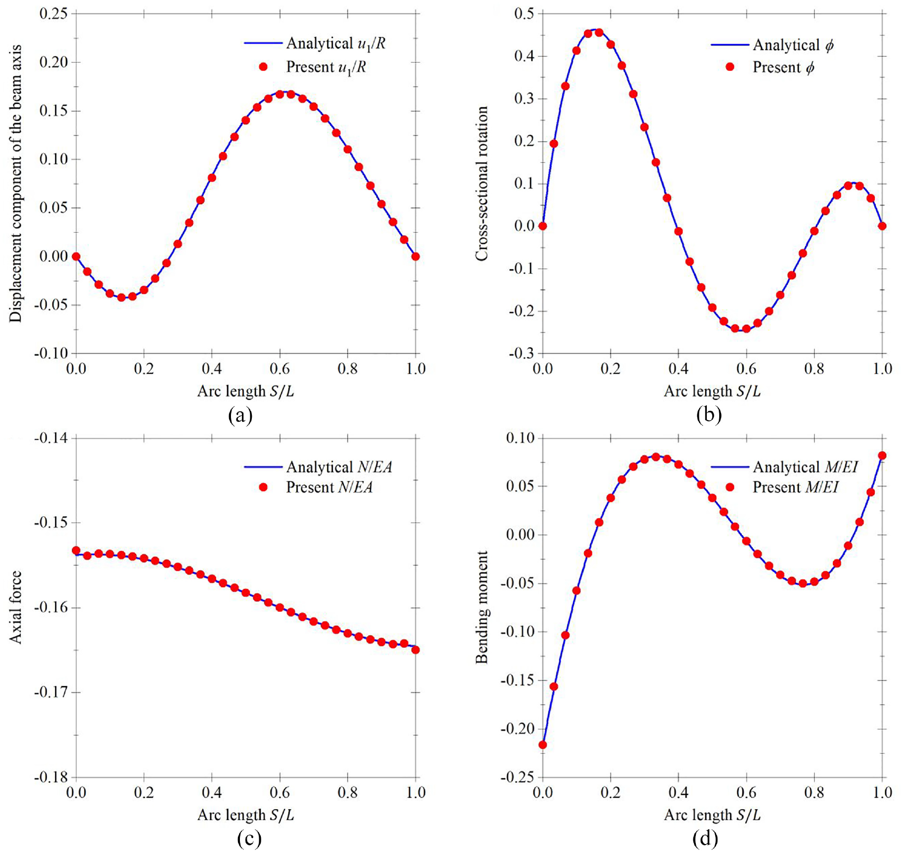
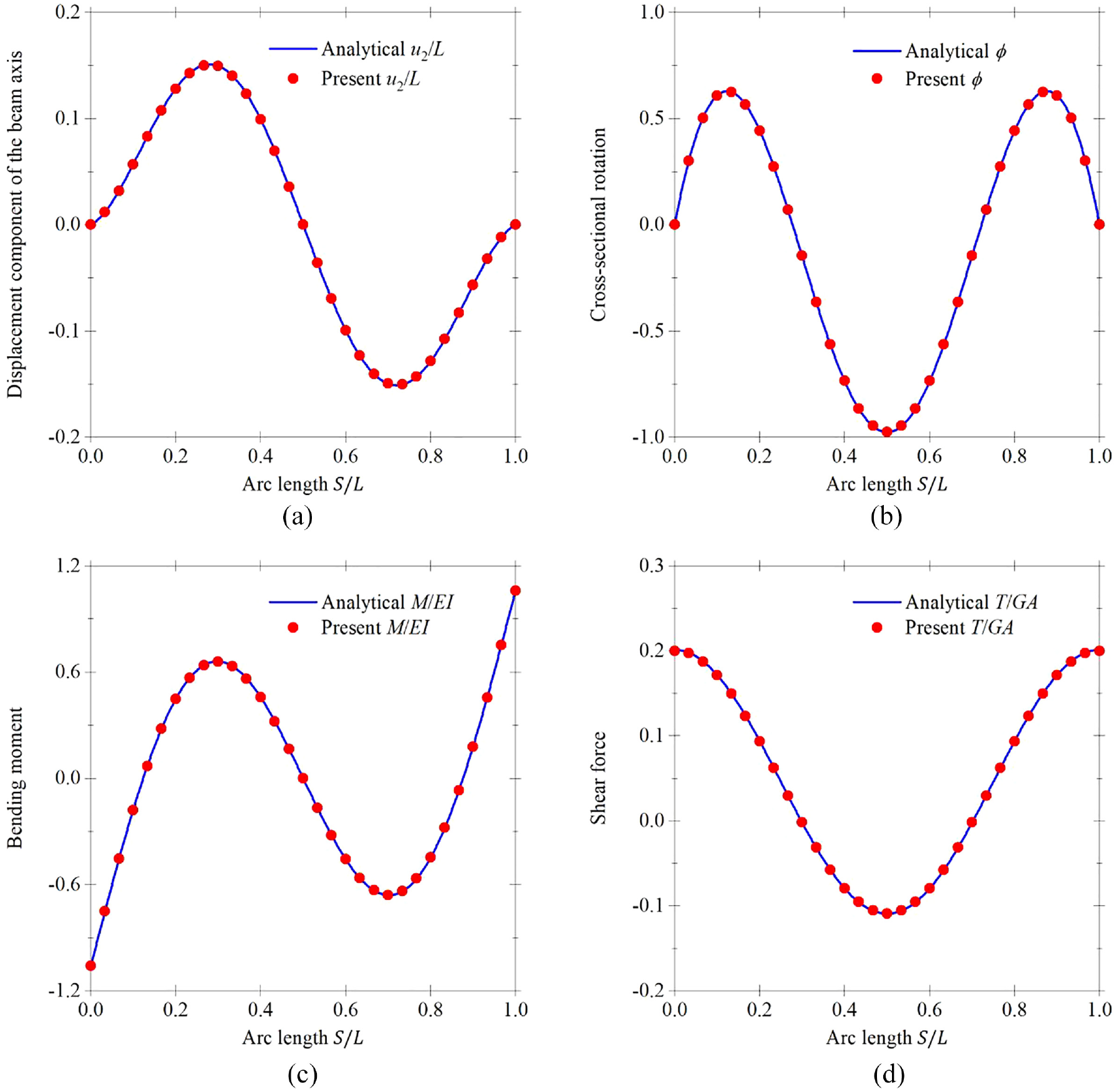
A semi-circular beam—numerical results with
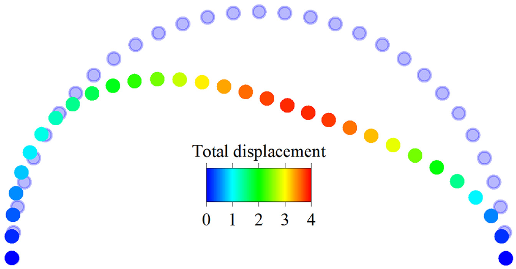
A semi-circular beam—Deformed configuration with
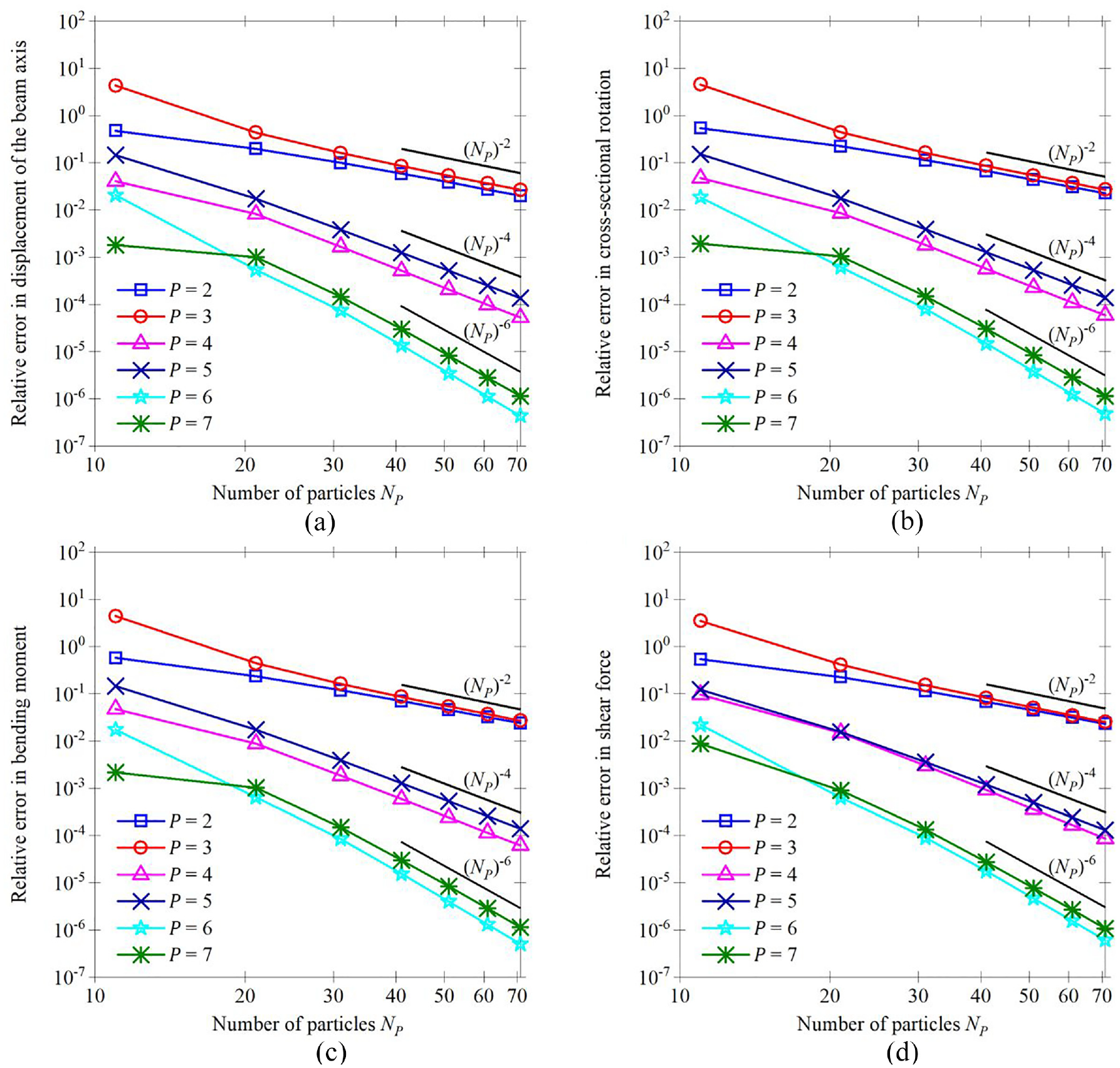
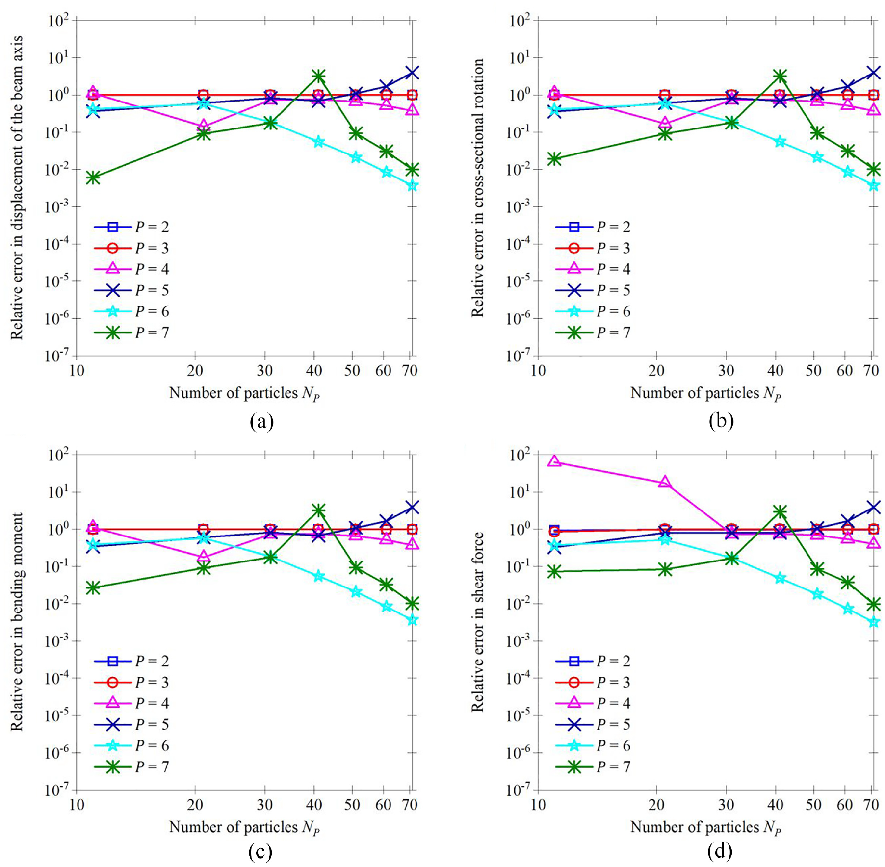
Convergence properties of the proposed formulation are further inspected with respect to the relative errors in the displacement of the beam axis, cross-sectional rotation, axial force, and bending moment. Since the analytical solutions of this example exist, they are used as reference ones for the calculation of relative errors. Convergence results with
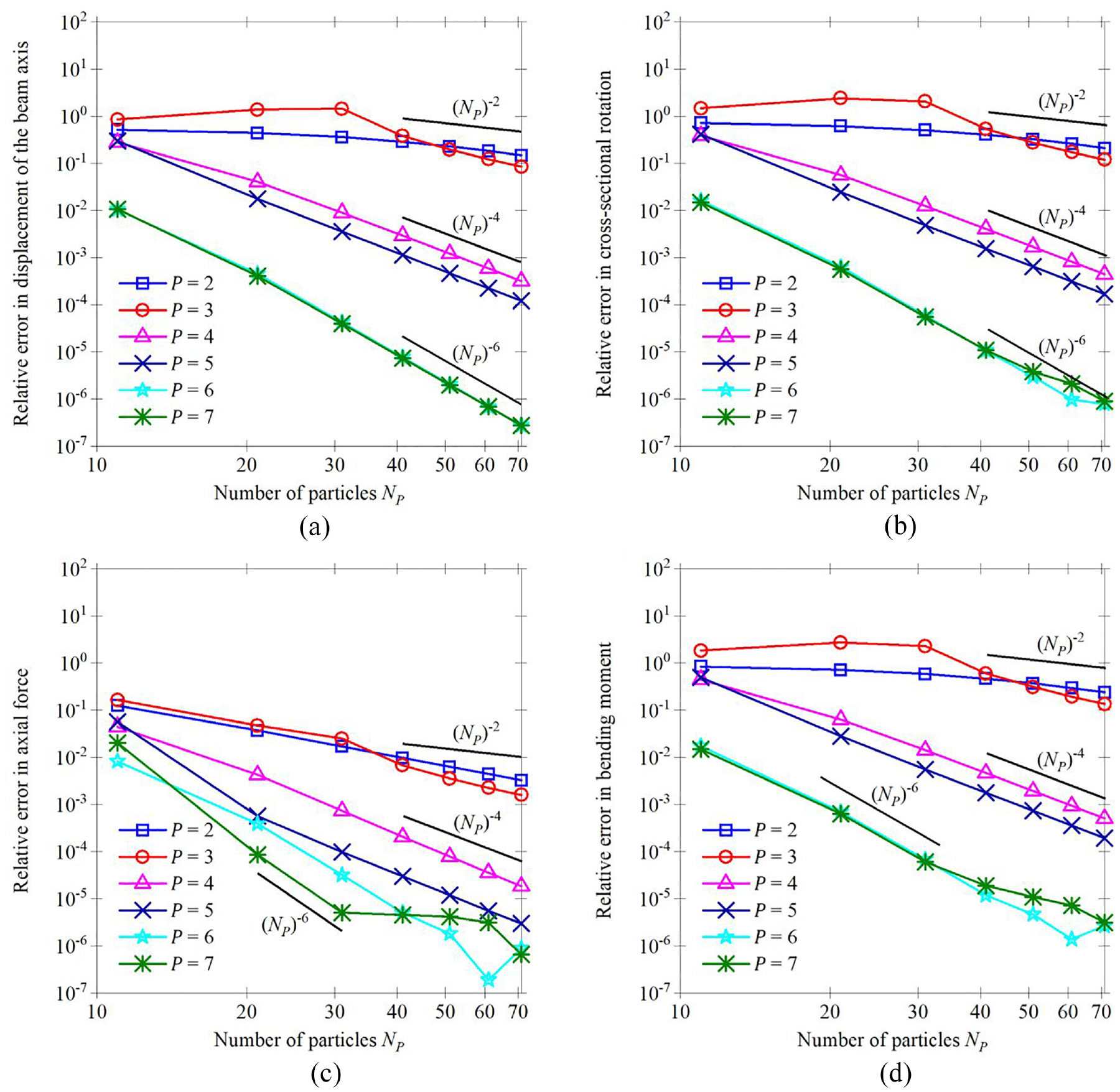
A semi-circular beam—convergence results with
Figure 11 portrays the deformed configuration with
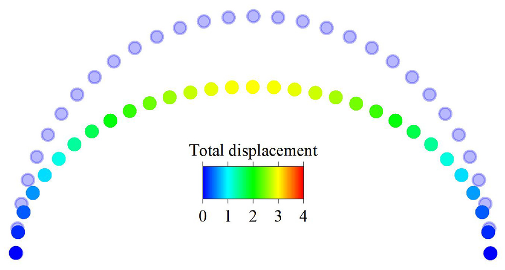
A semi-circular beam—deformed configuration with
The performance of the proposed formulation with
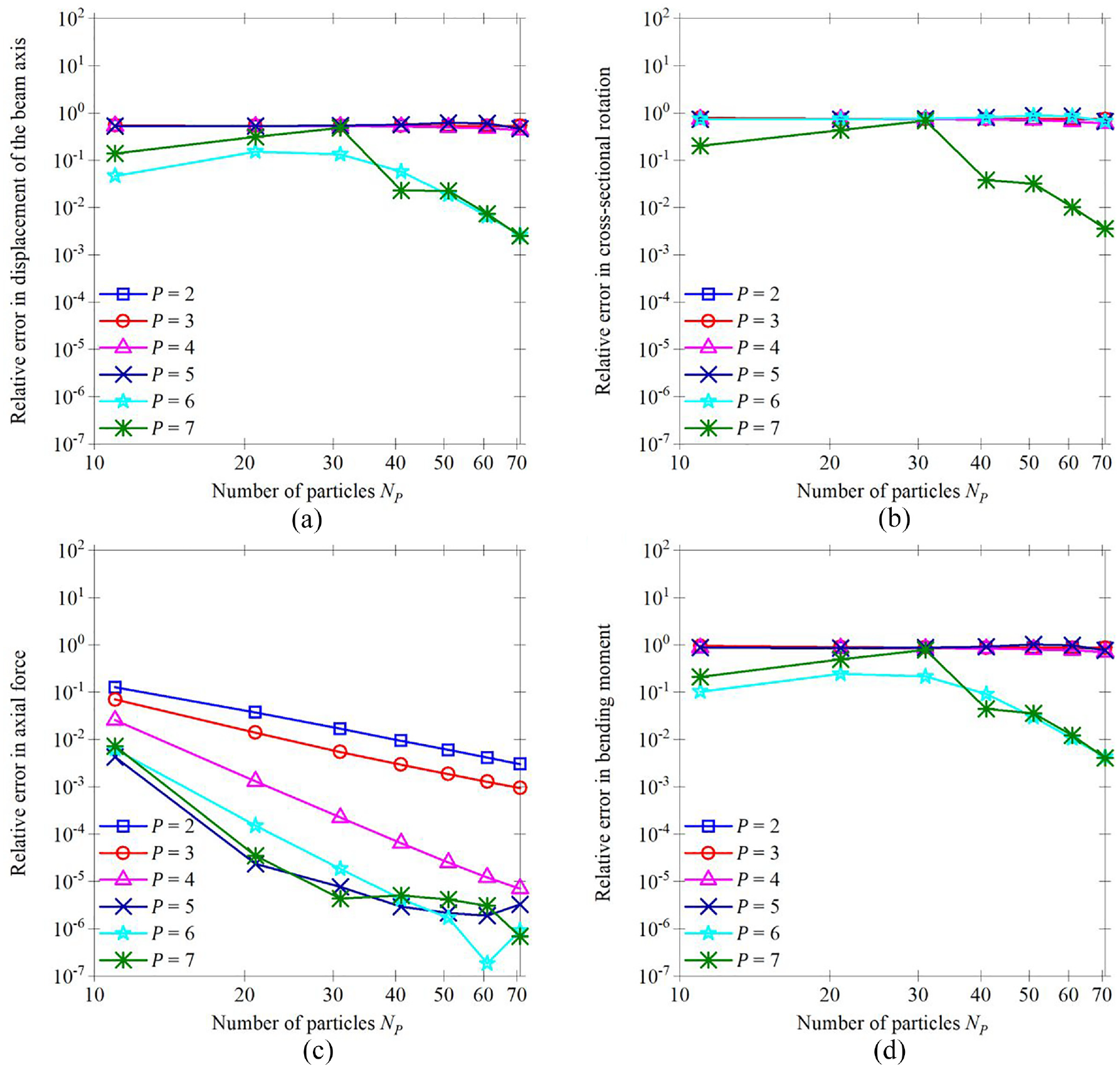
A semi-circular beam—convergence results with
A closer inspection reveals the deterioration in the convergence of the axial force with
4.3. A quintic beam
The two previous examples involve only simple beams having vanishing or constant curvature. In this last example, a quintic beam is considered to represent beams having arbitrary geometry. The geometrical configuration along with loading and boundary conditions are illustrated in Figure 13(a). The beam axis is described as follows:

with
A quintic beam. (a) Problem setup. (b) A peridynamic discretization.
For beams having beam axis with varying curvature, the equilibrium conditions contain non-constant coefficients, i.e., see Equations (14)–(16). Hence, it is challenging to derive analytical solutions for displacements and cross-sectional rotation if one prescribes boundary conditions and external loads. In fact, it is more straightforward to assign prior functions to displacements and cross-sectional rotation, and boundary conditions together with external loads are ascertained accordingly. These boundary conditions and external loads are then used for implementation of the proposed formulation, and the specified functions of the displacements and cross-sectional rotation are viewed as analytical solutions. In the coming tests, the displacements and cross-sectional rotation are specified as follows:
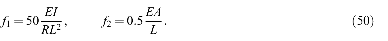
With the above functions, the beam is fixed at both ends, and the external loads are determined by substituting Equation (51) into Equations (14)–(16). Distributions of external loads are shown in Figure 14.
A quintic beam—external forces and moment with
The slenderness of the quintic beam is characterized by
A quintic beam—numerical results with
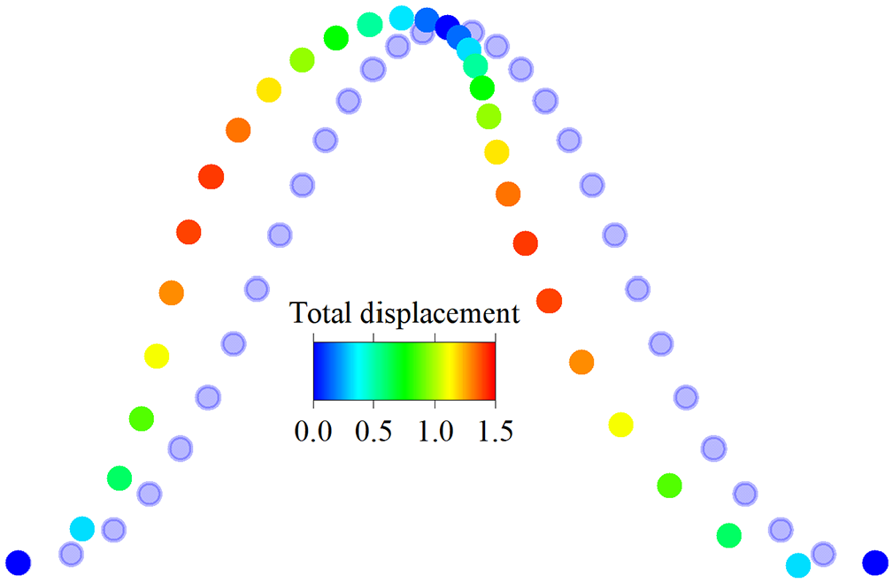
A quintic beam—deformed configuration with
To close this example, the examination on the sensitivity of the relative errors in the displacement of the beam axis with respect to the slenderness
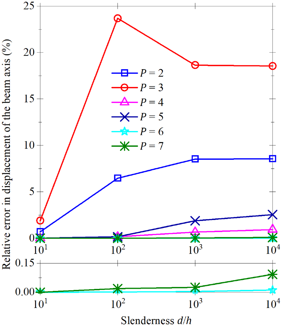
A quintic beam—relative error in displacement of the beam axis with different values of slenderness.
As a conclusive remark, membrane and shear locking effects are present in the numerical performance of the proposed formulation, but they can be significantly mitigated by utilizing peridynamic functions of higher polynomial degree.
5. Conclusion
This study presents a peridynamic formulation for the analysis of planar arbitrarily curved beams considering kinematic assumptions of Timoshenko–Ehrenfest beam model. Displacement components of the beam axis and rotation of the cross-section are used to describe linear kinematic relations. Equilibrium conditions and boundary conditions are derived by means of the principle of virtual work. Then, peridynamic functions are incorporated into the primal forms of equilibrium conditions to develop a peridynamic formulation.
Several rigorous tests are designed to assess the numerical performance of the proposed formulation. For relatively thick beams, the proposed formulation provides a good level of accuracy regardless of the highest polynomial degree used for the construction of peridynamic functions. However, the membrane and shear locking effects are found in the analysis of slender beams. In this scenario, it is suggested to utilize peridynamic functions of higher polynomial degree for the analysis of slender beams to ensure numerical precision. Indeed, the membrane and shear locking effects are significantly alleviated with the use of peridynamic functions of higher polynomial degree. Regarding the convergence properties, the order of convergence for even and odd values of
Footnotes
Appendix
Declaration of conflicting interests
The author(s) declared no potential conflicts of interest with respect to the research, authorship, and/or publication of this article.
Funding
The author(s) disclosed receipt of the following financial support for the research, authorship, and/or publication of this article: This Research is funded by Thailand Science research and Innovation Fund Chulalongkorn University (awarded to J.R.). This research project is supported by the Second Century Fund (C2F), Chulalongkorn University, Thailand (awarded to D.Vo). P.S. acknowledges partial support from Chiang Mai University, Thailand.
Data availability
The raw/processed data required to reproduce these findings cannot be shared at this time as the data also forms part of an ongoing study. Data will be made available on request.