Extended Dummy Node Rule for analysis and characterization of pin-jointed periodic cellular materials: An approach based on Bloch-wave method

Abstract

Micro-truss lattice materials are a class of hybrid periodic cellular solids that consist of a combination of solids and voids. The material is partitioned into cells structured in a given cell topology tessellated to form an almost unbounded micro-truss framework. The Bloch-wave method is one technique that can describe the propagation of a wave function over a periodic infinite lattice. It demonstrated the effectiveness of modeling the static and dynamic responses of lattices of various topologies. However, the Bloch-wave method presents limitations when applied to unit cell topologies whose structural elements extend across their envelopes to adjacent unit cells, as a given unit cell may not contain the full nodal parameters and periodicity information necessary to describe the kinematic and static wave propagations across the periodic lattice. The first part of this paper presents the Dummy Node Rule (DNR), which overcomes this limitation. The rule introduces dummy nodes at the intersection points between cell envelopes and elements extending between the adjacent unit cells, which are initially treated as part of the finite unit cell structure. Then, the rule establishes mathematical relationships between the static and kinematic wave functions propagating across dummy nodes and those propagating across the connected cell elements. The second part of the paper describes DNR for specific applications such as (a) the development of static and kinematic systems of the unit cell finite structure, which aids in the determinacy analysis of periodic lattice structures, and (b) the development of the Cauchy–Born kinematic boundary condition that is used to homogenize the kinematic response of the infinite periodic structure to an assumed macroscopic strain field, which in turn, forms the effective properties of the lattice material. Furthermore, the last part of the paper shows examples where the scheme is applied for the stiffness characterization of selected lattice topologies.

Keywords

Dummy Node Rule Bloch’s theorem Bloch-wave method Cauchy–Born hypothesis lattice structure lattice material periodic cellular solids periodic cellular materials infinite periodic structure

1. Introduction

The behavior of periodic cellular material, or lattice materials, can be determined by analyzing the kinematic determinacy of the pin-jointed version of the lattice microstructure [1,2]. The behavior can be primarily categorized into stretching- and bending-dominated [3 –6]. Maxwell [7] framed several guidelines to evaluate the kinematic determinacy, based on which a minimum number was set for the bars within a pin-jointed framework, to classify the behavior of the framework as stretching- or bending-dominated [8,9]. A framework with the minimum number of bars is characterized as stretching-dominated and, in the other case, as bending-dominated behavior, given that the nodes are rigid. In their work, Pellegrino and Calladine [10] conducted a comprehensive examination of the mathematical foundation of Maxwell’s rule, employing the kinematic matrices and related equilibrium subspaces in a pin-jointed arrangement. Their investigation led to an expanded version of Maxwell’s rule that incorporates insights into several aspects of the framework, such as the internal mechanisms and self-stress conditions. This generalized form of Maxwell’s rule enabled a precise assessment of the determinacy status of a finite structure, facilitating accurate predictions of truss-like structural behavior.

Periodic cellular materials have a microscale structure and, at the same time, can be incorporated into a macroscale structure considering their homogenized mechanical characteristics [11 –13]. The approach is much developed and applicable for engineered materials such as mechanical metamaterials [14], where lower-scale microstructures are designed for specific tailored functionalities. The use of homogenization methods for predicting vibrations in unbraced periodic frames of discrete media was demonstrated in earlier works [15,16], to evaluate behavior at the level of first-order terms. The scope of the study included deformation effects due to gravity, soil-structure interaction, and coupled transverse-longitudinal vibrations. The homogenization of periodic discrete media was also extended [16] for analyzing the dynamics of one-dimensional (1D) structures, starting from the point of a static strain applied to the level of the single cell. In another approach [17], 1D periodic model based on Timoshenko beam theory was established to study the static and dynamic behaviors, taking into the effect of micro-warping. A homogenization technique based on energy equivalence between the analyzed micro-structured grid beam and a developed equivalent beam subjected to similar displacement field. The methodology was also expanded [18] for conducting the buckling analysis study of uniformly compressed micro-structured grid beams based on the 1D approach.

The assumption of periodicity in an unbounded domain of the material microstructure necessitates an extension of the determinacy analysis to fully capture the behavior of cellular material as the domain of analysis is at the scale of the infinite lattice [19 –24]. This extension by Despande et al. [4] focused on a particular class of lattice structures with all nodes similarly situated in a spatial dimension, that is, the lattice is invariant when seen from any point around a node regardless of the viewpoint. However, only specific topologies, including the square and the fully triangulated lattices in two-dimensional (2D) cases and octet-truss in the case of three-dimensional (3D) geometries, fulfilled this. More recently, based on Bloch’s theorem, Hutchinson and Fleck [37] modeled the wave propagation in a lattice structure characterized by their infinite periodicity and with any Bravais symmetry. Their approach could comprehensively capture the infinite lattice’s internal mechanisms and self-stress states. Furthermore, they have illustrated how the results of the determinacy analysis influence the lattice performance at a macroscopic scale. Their work mainly considered topologies where the cell elements’ end nodes lay on the envelope boundaries. An example of this type of lattice structure is the Kagome lattice as shown in Figure 1(a). However, topologies, such as those shown in Figure 1(b)–(h), do not possess the complete nodal parameters and periodicity information required by the static and kinematic analyses using Bloch’s wave method. Such information is essential for (a) the homogenization of the infinite periodic structure mechanical characteristics, using the kinematic boundary condition formulation based on the Cauchy–Born hypothesis (CBH) [25 –29] and (b) the establishment of the characteristics of the unit cell, such as its static and kinematic systems [30,31].

Figure 1.

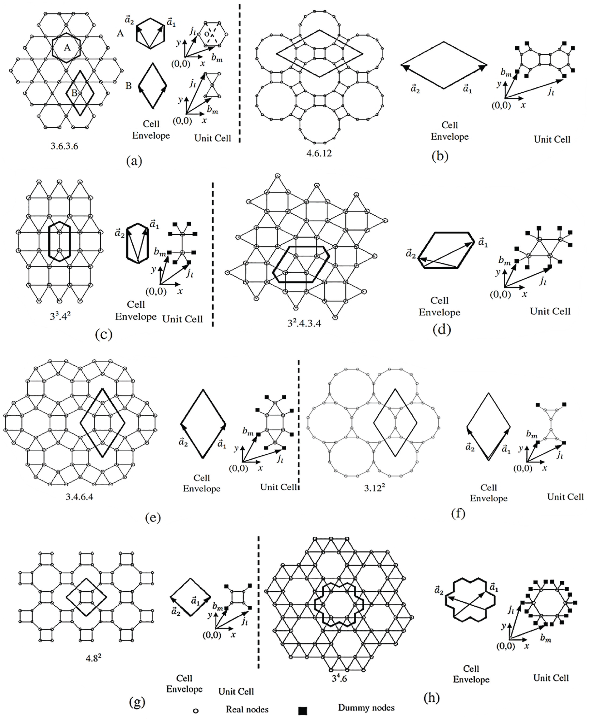
2D lattice structures: (a) Kagome 3.6.3.6, (b) 4.6.12, (c) 3³.4², (d) 3².4.3.4, (e) 3.4.6.4, (f) 3.12², (g) 4.8², and (h) 3⁴.6 [32].

The paper extends the kinematic and static analyses of periodic cellular materials to topologies where the envelope intersects the cell elements at points beyond the cell nodes. To achieve this objective, we propose implementing a guideline that mandates the inclusion of dummy nodes at the junctions where the envelope of the unit cell coincides with its constituent elements in what we call the Dummy Node Rule (DNR). By leveraging Bloch’s theorem, the DNR facilitates the study of the static and kinematic waves through the cell elements and the dummy nodes related to them. The DNR utilizes a linear interpolation technique to establish the mathematical relationships connecting the wave functions propagating associated with the real and the dummy nodes of the lattice. The determinacy of the material microstructure and the characterization of the material’s effective properties are evaluated by applying the developed DNR technique. It is to be highlighted that while periodicity can be developed based on high-fidelity model elements such as bricks and voxels, based on conventional numerical techniques such as finite element method (FEM), a low-fidelity model based on frame and truss elements established in the following concept cannot be established without the DNR approach. Therefore, the DNR approach is a stride toward attaining computational efficiency and enables faster processing of complex lattice structures. A simple scheme is presented for the application of the DNR. The proposed methodology entails the utilization of dummy nodes for the formulation of the nodal deformations of the unit cell, which can be derived with respect to a macroscopic homogeneous strain field, which is also followed by the CBH [33] and the features of the unit cell associated with the finite microstructure such as the equilibrium and kinematic matrices. After the establishment of the matrix system, the modes and the degrees of freedom (DOF) related to the dummy nodes, captured in the column and row spaces of the matrices of the kinematic and equilibrium conditions, respectively, are eliminated generating the final matrix expressions of the original structure without the hypothetical dummy nodes.

The paper is mainly organized into six sections. After this introduction, the mathematical description of an infinite lattice structure is presented. The third section states the DNR and presents its proof. The fourth section introduces the elimination scheme and presents its proof. The fifth section details how the DNR scheme can be applied in the stiffness characterization of selected lattice topologies. The last section summarizes the study with a concluding outlook on the capability of the scheme [32]. The approach aids in the process of design and evaluation, by predicting the performance of complex lattice structures [34], with tuned topologies and geometries.

2. Mathematical description of a lattice structure

The microstructures considered in this study are based on Euler–Bernoulli’s beam-column formulation, where the unit cell is considered a finite structure of elastic beams and rigid joints. However, it is to be noted that the analysis does not take into account any buckling deformation. The finite structural problem is then converted to a periodic case of infinite extent by assuming that Bloch’s theorem can represent the infinitesimal value of the displacement field at the rigid-joint point, otherwise, known as the node.

The initial example used in the analysis is that of a 2D square lattice structure, as illustrated in Figure 2. The thin lines describe the lattice, whereas the thick lines represent the cell envelopes. It is to be noted that unit cells A and B can produce a square lattice through a 2D infinite tessellation [32,35,36]. Based on the method developed by Hutchinson and Fleck [37], unit cell A can be selected for a comparatively simpler route to characterizing and analyzing the state of determinacy of the square lattice. On the contrary, the same analysis, which utilizes Bloch’s wave procedure, becomes complicated and challenging in the case of unit cell B, as there are no end nodes of the unit cell lying on the envelope to form the required lattice periodicity. The procedure utilizing unit cell B affects the derivation of the static and kinematic systems, which also influences the kinematic boundary condition. The kinematic boundary condition and related details are vital in developing a homogenization methodology for the mechanical properties related to the lattice microstructure. These are achieved as a result of the derivation based on the CBH. Although unit cell B can be avoided and unit cell A can be selected for the square lattice, for other lattice topologies—such as those shown in Figures 1(b)–(h), this strategy might not be possible.

Figure 2.

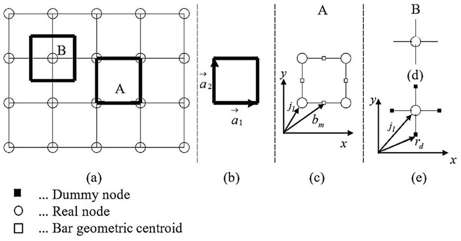
(a) lattice structure, (b) cell envelope, (c) unit cell A, (d) unit cell B without dummy nodes, and (e) unit cell B with dummy nodes [32].

In this paper, we introduce the DNR to evaluate the lattice topologies of the type as shown in Figure 1(b)–(h). The methodology of DNR requires a set of parameters to be defined that describe the microscopic constituents of a lattice structure and aid in modeling wave-function propagation across the infinite lattice structure. These parameters describing the lattice structure are illustrated in Figure 2 and are explained below.

2.1. Lattice bases

The lattice structure can be differentiated into two distinct groups of bases, that is those of the node and bar bases groups [2,38]. The position vectors are utilized to represent both sets of bases. Each unit cell, as depicted in Figure 2, has a specific Cartesian coordinate system defined for accurate representation. The point of coordinate system origin is situated at the lower-left vertex in the case of unit cell A, while on the contrary, for unit cell B, it will be located at the one real node available. It is to be noted that the position vectors $j$ and $r$ are associated with the real and dummy nodes, respectively, whereas the vector $b$ indicates position of the geometric centroid of the bar element. An assumption is made that all the constituent microscopic cell elements of the square lattice have a unit value of length $(L = 1)$ . Section 2.1.1. highlights the prime feature of the present investigation, which is introducing an additional bases group of dummy nodes.

2.1.1. Dummy Node Bases Group

The cell elements forming the constituent unit cells of a given lattice may not have their end nodes coinciding with the defined cell envelope. In such cases, the artificial dummy nodes, as indicated in Figure 2(e), are placed at the junctions where the envelope of the unit cell coincides with the constituent cell elements.

The mathematical group, G_D, is defined as the bases group of all the dummy nodes consisting of all its position vectors $r_{d} \equiv j_{d}$ , with $D$ being the number of dummy nodes and $d \in {1, \dots, D}$ , all described at the level of a unit cell.

In the case of the two-unit cells considered, unit cell A is characterized by

$G_{D}^{A} = Ø$ , with Ø being an empty group.

On the contrary, the same group for unit cell B can be defined:

$G_{D}^{B} = {(- 0.5, 0), (0, 0.5), (0.5, 0), (0, - 0.5)}$ .

It is to be noted that for each of the terms defined for the respective case, the superscript indicates the unit cell to which it belongs.

2.1.2. Node Bases Group

The position vectors for each node in a unit cell are collected in a mathematical group called the node bases group $G_{N}$ . Depending on the nature of the nodes defined within a unit cell, the formulation of the node bases group varies.

For the case of unit cell A, as illustrated in Figure 2(c), where the unit cell solely comprises real nodes, the node bases group is defined as:

$G_{N} \equiv {j_{1, \dots}, j_{l, \dots}, j_{j}}$ .

where $j$ is the number of nodes and $j_{l}$ is the position vector of a node $l$ defined in space $l \in {1, 2, . . . j}$ .

Considering unit cell A, its node bases group can be described as:

$G_{N}^{A}$ $= {(0, 0), (0, 1), (1, 1), (1, 0)}$

As shown in Figure 2(e), for unit cell B consisting of dummy nodes, its node bases group is expressed as:

$G_{N} \equiv {j_{1}, . . ., j_{l}, . . ., j_{j}} \cup G_{D}$ .

Therefore, for unit cell B, the node bases group can be described as

$G_{N}^{B} = {(0, 0), (- 0.5, 0), (0, 0.5), (0.5, 0), (0, - 0.5)}$ .

A.3 Bar Bases Group

The position vectors for each bar in a unit cell are collected in a mathematical group called the bar bases group $G_{B}$ .

For unit cell A, consisting solely of real nodes, its bar bases group is defined as:

$G_{B} \equiv {b_{1}, . . ., b_{m}, . . ., b_{b}}$ .

where $b$ is the number of bar elements connecting real nodes, and $b_{m}$ is the position vector of the geometric centroid concerned with the bar, given $m \in {1, 2, . . . b}$ .

For unit cell A, its bar bases group can be written as:

$G_{B}^{A} = {(0, 0.5), (0.5, 1), (1, 0.5), (0.5, 0)}$ .

In the case of unit cells containing dummy nodes, such as unit cell B, it is noted that the connecting bars’ position vectors and the dummy nodes’ position vectors coincide, and therefore, $G_{B} \equiv {b_{1}, . . ., b_{m}, . . ., b_{b}} \cup G_{D}$ .. Hence, it is apparent that the bases groups of the bars and nodes form a subset of the dummy node bases.

For unit cell B, the bar bases group is then can be expressed as:

$G_{B}^{B} = {(- 0.5, 0), (0, 0.5), (0.5, 0), (0, - 0.5)}$ .

2.2. Direct translational bases

The cell tessellation process is regulated by the translational bases, which are classified based on the dimension of the analysis. It is indicated by ${\vec{a}}_{k}$ , where $k \in {1, 2}$ for 2D cases, and termed as lattice symmetry primitive bases, whereas the term direct translational bases are used for the 3D cases, with $k \in {1, 2, 3}$ .

For example, the two vectors ${\vec{a}}_{1}$ and ${\vec{a}}_{2}$ , as shown in Figure 2(b), are direct translational bases related to the envelope enclosing a unit cell. Figure 2(c) and Figure 2(e) illustrates these direct translational bases for the respective cases of unit cells A and B. As depicted in Figure 2(a), these two vectors are used in a translational symmetry to construct the desired infinite square lattice structure. In the case of both the unit cells, it can be deduced that ${\vec{a}}_{1} = (1, 0)$ and ${\vec{a}}_{2} = (0, 1)$ .

2.3. Direct translational vector

The direct translational vector accomplishes the translation of the reference unit cell within the lattice space through a linear combination of the direct translational bases. The vector can be expressed as:

\vec{R} = \sum_{k = 1}^{n} m_{k} {\vec{a}}_{k} .

(1)

where k ∈ ${1, \dots, n}$ is the dimensional space for the lattice structure, with $n$ = 2 or 3 for the 2D and 3D cases, respectively. Here, $m_{k}$ is any integer set forming the linear combination of the direct translational bases.

2.4. Position vectors

The reference unit cell attributes, such as nodal, bar, and direct translational bases, can be used to establish a set of defining parameters. The following definition can be set for the position vectors of the constituent nodes and bar elements for the lattice structure.

Considering the entire lattice structure, the position vectors of the nodes and those of the bars can be formulated by defining the bases of the nodes and bars and the direct translational bases related to a reference unit cell. It can be expressed as:

p_{l} = j_{l} + \vec{R} = j_{l} + \sum_{k = 1}^{n} m_{k} {\vec{a}}_{k} . l \in {1, . . ., J} .

q_{m} = b_{m} + \vec{R} = b_{m} + \sum_{k = 1}^{n} m_{k} {\vec{a}}_{k} . m \in {1, . . ., B} .

(2)

where $k \in {1, \dots, n}$ is the dimensional space for the lattice structure, with $n$ = 2 or 3 for the 2D and 3D cases, respectively, given the relation $m_{k} \in Z$ remains constant. Here, $p_{l}$ and $q_{m}$ denote the position vectors for the respective node and bar, whereas $B$ and $J$ indicate the number of independent bars and nodes, respectively, for a given unit cell.

The derivation for the independent set of bases will be explained in Section 2.5.

2.5. Direct lattice

It is a set of infinite bases consisting of the independent node and bar bases set over the envelope of the reference unit cell, extended by the position vectors across an infinite periodic lattice. Therefore, the dependency of the bases is critical and is evaluated by the following formula with respect to a reference unit cell.

V_{i - 1} = V_{i} + \sum_{k = 1}^{n} {\hat{x}}_{k} {\vec{a}}_{k} .

(3)

where ${\hat{x}}_{k} \in {- 1, 0, 1}$ is the translation vector of unit magnitude. Here, $V_{i - 1}$ and $V_{i}$ are values that vary depending on the point of reference, that is, node and bar.

For the case of bars:

$V_{i} \equiv b_{m}$ and $i \equiv m \in {1, . . ., B}$ illustrate the bar position vector.

On the contrary, in the case of nodes:

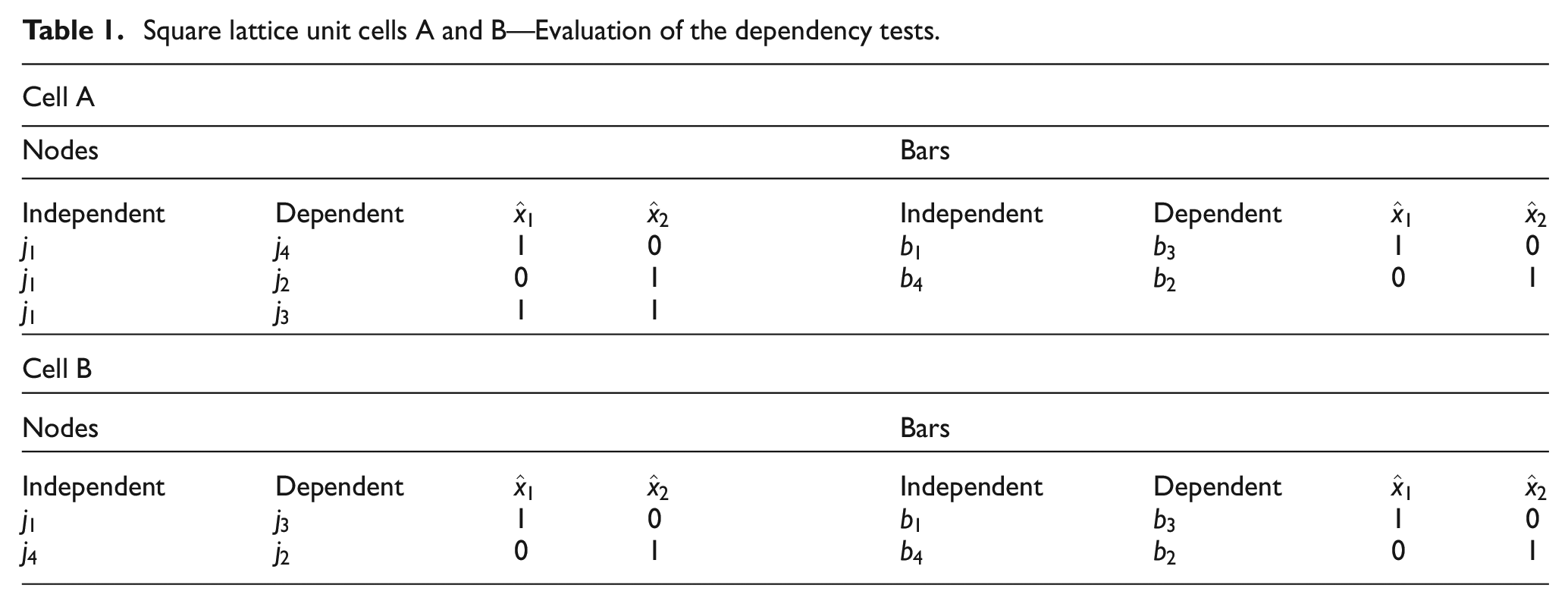
$V_{i} \equiv j_{l}$ and $i \equiv l \in {1, . . ., J}$ illustrate the node position vector.

It is to be noted that, for an infinite lattice structure, the above-derived dependency details are pivotal in determining the periodic wave function varying across the structure and can be obtained through the initial modification of the function related to the reference unit cell. Considering unit cells A and B, the obtained dependency relations are stated in Table 1.

Table 1.

Square lattice unit cells A and B—Evaluation of the dependency tests.

Cell A
Nodes				Bars
Independent	Dependent	${\hat{x}}_{1}$	${\hat{x}}_{2}$	Independent	Dependent	${\hat{x}}_{1}$	${\hat{x}}_{2}$
$j_{1}$	$j_{4}$	$1$	$0$	$b_{1}$	$b_{3}$	$1$	$0$
$j_{1}$	$j_{2}$	$0$	$1$	$b_{4}$	$b_{2}$	$0$	$1$
$j_{1}$	$j_{3}$	$1$	$1$
Cell B
Nodes				Bars
Independent	Dependent	${\hat{x}}_{1}$	${\hat{x}}_{2}$	Independent	Dependent	${\hat{x}}_{1}$	${\hat{x}}_{2}$
$j_{1}$	$j_{3}$	$1$	$0$	$b_{1}$	$b_{3}$	$1$	$0$
$j_{4}$	$j_{2}$	$0$	$1$	$b_{4}$	$b_{2}$	$0$	$1$

2.6. Reciprocal lattice

The primary utilization of a Bravais lattice—otherwise termed a reciprocal lattice, is when a lattice structure is expressed in the form of its lattice vectors. Utilizing this adoption has the benefit of discretizing the continuous lattice space so that the lattice performance can be evaluated at the discrete summation of modes.

Primitive vectors indicated by $\vec{b_{1}}$ and $\vec{b_{2}}$ characterize the reciprocal lattice and are defined by the following relation:

{\vec{b}}_{i} . {\vec{a}}_{j} = 2 π δ_{ij} .

(4)

where ${\vec{a}}_{j}$ is the direct lattice bases, and ${\vec{b}}_{i}$ indicates the reciprocal lattice bases. $δ_{ij}$ symbolizes the Kronecker delta function with:

δ_{ij} = {\begin{matrix} 0 for i \neq j . \\ 1 for i = j . \end{matrix}

(5)

where $i, j \in {1, 2}$ for 2D cases.

For the reciprocal lattice, the definition of the translational vectors is as follows:

ω = ω_{1} {\vec{b}}_{1} + ω_{2} {\vec{b}}_{2} . ω_{1}, ω_{2} \in [0, 1) \subset Q .

(6)

where $ω_{1}$ and $ω_{2}$ are covariant components of $ω$ with respect to the basis ${\vec{b}}_{1}$ and ${\vec{b}}_{2}$ . $Q$ denotes a set of rational numbers.

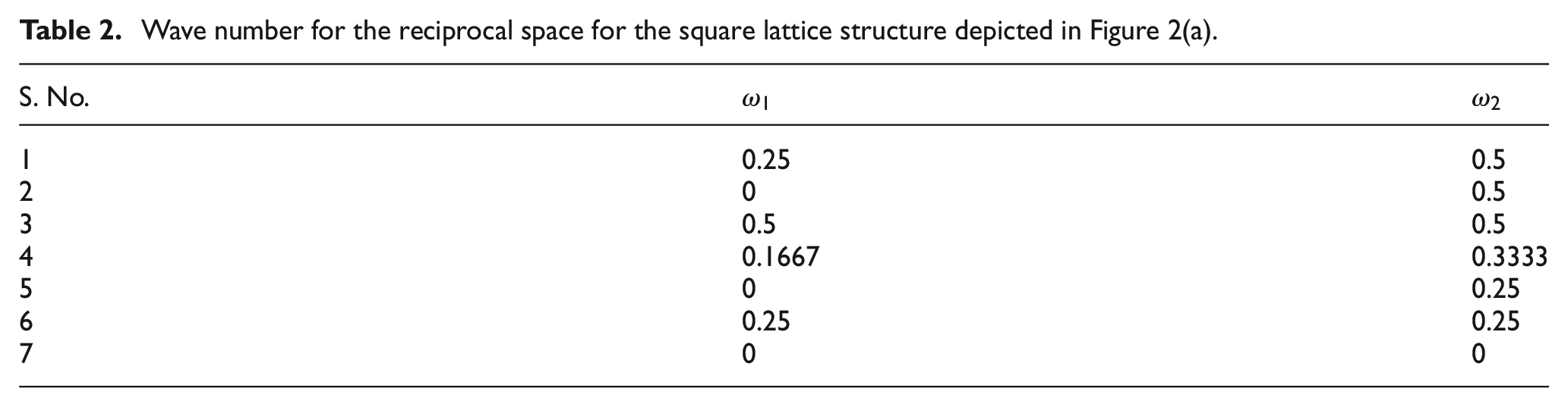
The first irreducible Brillouin zone (IBZ) [39 –41] was utilized along with Bloch’s theorem [42] of the reciprocal lattice to derive the values of $ω_{1}$ and $ω_{2}$ . Section 2.7 provides a brief description of Bloch’s theorem.

Reciprocal lattice bases are calculated as ${\vec{b}}_{1} = (1, 0)$ and ${\vec{b}}_{2} = (0, 1)$ for the square lattice illustrated in Figure 2(a). The wave numbers and the related IBZ are illustrated in Table 2 and Figure 3, respectively.

Table 2.

Wave number for the reciprocal space for the square lattice structure depicted in Figure 2(a).

S. No.	$ω_{1}$	$ω_{2}$
1	0.25	0.5
2	0	0.5
3	0.5	0.5
4	0.1667	0.3333
5	0	0.25
6	0.25	0.25
7	0	0

Figure 3.

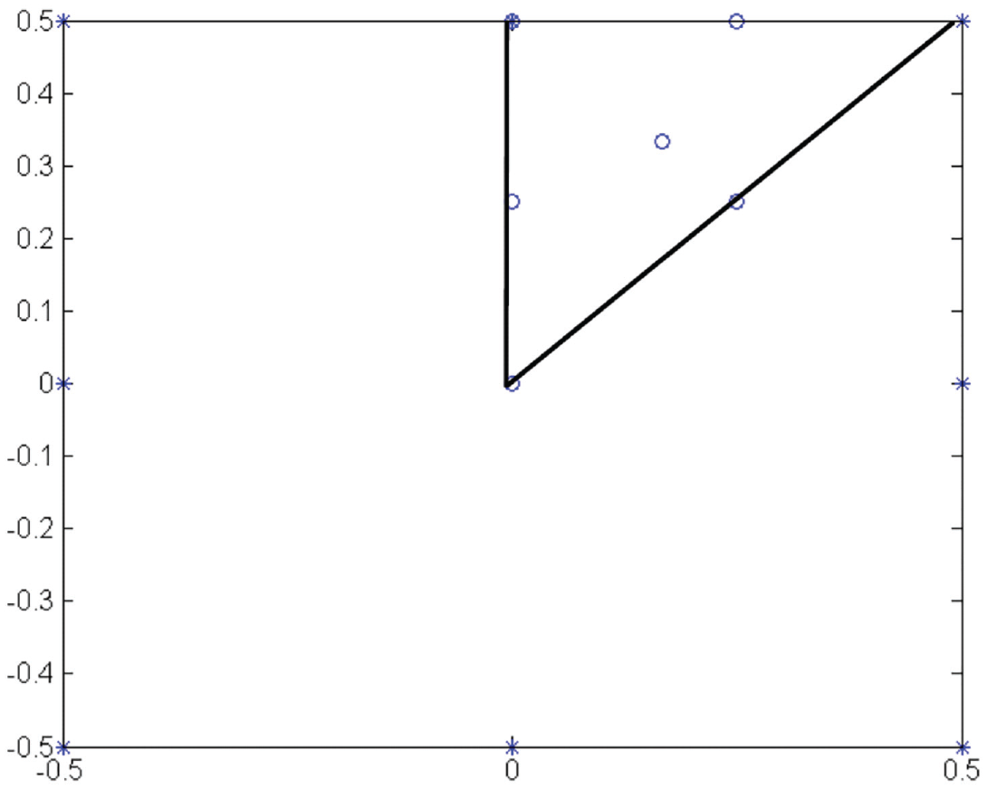
Square lattice structure indicated in Figure 2(a)—First Brillouin zone and IBZ.

2.7. Bloch’s theorem

The unit cell analysis of the earlier sections can be extended to the level of unbounded periodic lattice using Bloch’s theorem [21,43 –45].

2.7.1. Bloch wave function

Bloch’s theorem is applied to define the propagation of a wave function over the infinite lattice structure. The generalized form of the nodal displacement vectors $d (p_{l}, ω) \in C^{2}$ , for a given function of the nodal deformation value, can be expressed over the entire lattice as a wave function of the form:

d (p_{l}, ω) = d (j_{l} + \vec{R}, ω) d (j_{l}, ω) ex p^{2 π i ω \vec{R}} . l \in {1, 2, \dots ., J} .

(7a)

where $p_{l} = j_{l} + \vec{R}$ is the position vector of any node within the lattice. Here, $\vec{R}$ is the Bravais cell vector of any unit cell through the entire lattice, and $J$ is the number of independent nodes within the unit cell envelope.

Similarly, for the bar deformation function, the generalized bar deformation vectors $e (q_{m}, ω) \in C^{2}$ can be expressed over the entire lattice as a wave function of the form:

e (q_{m}, ω) = e (b_{m} + \vec{R}, ω) = e (b_{m}, ω) ex p^{2 π i ω \vec{R}} . m \in {1, 2, . . ., B} .

(7b)

where $q_{m} = b_{m} + \vec{R}$ is the position vector of any bar within the lattice, and $B$ denotes the number of independent bars with respect to the unit cell.

3. The DNR

To tessellate a unit cell into an infinite periodic lattice structure, three main bases groups are utilized, namely

$G_{N}$ denoting the node bases group.

$G_{B}$ denoting the bar bases group.

$G_{D}$ denoting the dummy node bases group, with $G_{D} \subset G_{N}$ .

For a pair of real nodes $k$ and dependent dummy node $l$ , with position vectors $j_{k} \in G_{N}$ and $j_{i} \equiv b_{m} \in G_{D}$ , respectively, consider a dependent bar element $m$ connecting them. Similarly, for a pair of real nodes $l$ and independent dummy node $j$ with position vectors $j_{l} \in G_{N}$ and $j_{j} \equiv b_{n} \in G_{D}$ , respectively, consider an independent bar element $n$ connecting them. According to the DNR, for each independent bar element $n$ , there exists a bar element $m$ which is dependent in nature with the following conditions:

t_{m} = - t_{n} ex p^{2 s π i ω} .

(a)

f_{i} = - f_{j} ex p^{2 s π i ω} .

(b)

e_{m} = e_{n} ex p^{2 s π i ω} = e_{m 1} + e_{n 2} ex p^{2 s π i ω} = e_{m 2} + e_{n 1} ex p^{2 s π i ω} .

(c)

d_{i} = d_{j} ex p^{2 s π i ω} .

(d)

d_{i} = (d_{l} ex p^{2 s π i ω} - d_{k}) \frac{‖ j_{i} - j_{k} ‖}{‖ j_{l} + s a_{k} - j_{k} ‖} .

(e)

d_{j} = (d_{l} - d_{k} ex p^{- 2 s π i ω}) \frac{‖ j_{l} - j_{j} ‖}{‖ j_{l} + s a_{k} - j_{k} ‖} .

(f)

where $Ω$ is the value of a wave number obtained from the lattice IBZ. Here, $i = \sqrt{- 1}$ is the imaginary unit of a complex number, and $s$ is the periodicity within the cell envelope. It is a unit integer where $s \in {1, - 1}$ , and as shown in Equation (3) with the relation $s \subset {\hat{x}}_{k}$ existing constant. Also, ${\vec{a}}_{k}$ is the direct translational basis of the lattice, $d$ is the nodal displacement value, $e$ is the elemental axial deformation value, $f$ is the nodal force value, and $t$ is the elemental tension force value.

The subscripts described in the above set of equations include $i$ —associated with dummy node; $j$ —associated with dummy node $j$ ; $m$ —associated with element $m$ ; $n$ —associated with element $n$ ; $m_{1}$ —part of element $m$ in the envelope of the reference unit cell; $m_{2}$ —part of element $m$ not included within the envelope of the reference unit cell; $n_{1}$ —part of element $n$ in the envelope of the reference unit cell, and $n_{2}$ —part of element $n$ not included within the envelope of the reference unit cell.

It is worth mentioning that, due to the lattice’s translational symmetry, the introduction of dummy nodes occurs exclusively in pairs. The two dummy nodes are periodically interdependent within each pair with a one-step integer translation, as outlined by Equation (3).

3.1. Proof of the DNR

The lattice arrangement, depicted in Figure 4, consists of three-unit cells and involves the elements $m$ and $n$ . The node $k$ , situated between the first- and second-unit cells, is linked to element $m$ and node $p$ , which is located within the third unit cell. The nodes $q$ and $l$ , located in the first- and second-unit cells, respectively, are linked to element $n$ . Two dummy nodes, $i$ and $j$ , are placed at the intersection of the envelope of the second unit cell with the elements $m$ and $n$ , respectively. Element .is separated into element $m 1$ , having length $L_{m 1}$ , and element $m 2$ of length $L_{m 2}$ by node $i$ . In a similar manner, element $n$ is divided into element $n 1$ , having a length of $L_{n 1}$ , and element $n 2$ of length $L_{n 2}$ by the node $j$ . The elements denoted as $m$ and $n$ are subjected to internal tension forces, represented by $t_{m}$ and $t_{n}$ , respectively. For the elements $m$ and $n$ , the nodal force part balancing the tension forces is represented as $f_{r}$ , which is a 2D vector, $r \in {i, j, k, l, p, q}$ .

Figure 4.

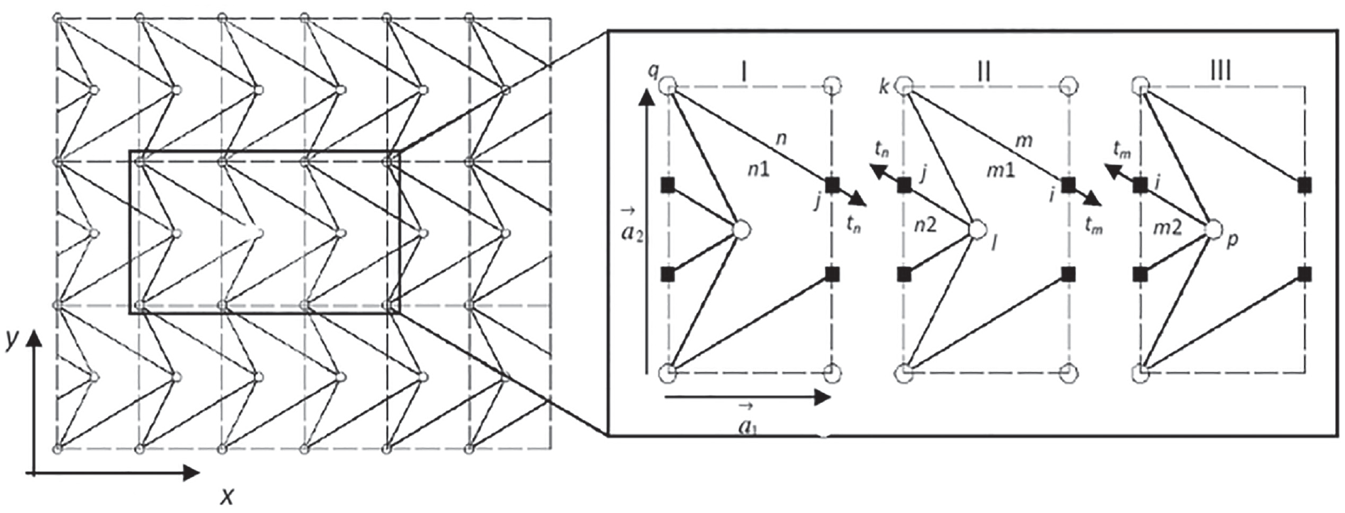
A structural arrangement of the lattice (shown in the left figure) and three constituent unit cells (shown in the right inset figure). Based on the horizontal translational basis, these unit cells are tessellated to form the entire structure. The dashed lines denote the cell envelopes, whereas the continuous lines denote structural components. The real and dummy nodes are denoted as (O) and (■), respectively [32].

It can be inferred that element $m$ has a periodic dependency relation with element $n$ from a geometric examination of the three-unit cell assembly illustrated in Figure 4. As a result, the following formulation may be used to express the connection between the position vectors of the node and bar elements:

j_{i} = j_{j} + {\vec{a}}_{1} .

(8)

b_{m} = b_{n} + {\vec{a}}_{1} .

(9)

{\hat{n}}_{m} = {\hat{n}}_{n} .

(10)

By utilizing the bar dependency relationship as outlined in Equation (9), it is possible to apply Bloch’s theorem to express the wave functions that propagate throughout cell elements in terms of specific force and deformation components. The expressions for the axial deformation and tension force components experienced by elements $m$ and $n$ are stated as follows:

t_{m} = t_{n} ex p^{2 π i ω} .

(11)

e_{m 1} = e_{n 1} ex p^{2 π i ω} .

(12)

e_{m 2} = e_{n 2} ex p^{2 π i ω} .

(13)

By dividing the assembly of three-unit cells into individual cells, as depicted in Figure 4, and utilizing the principles of static equilibrium while specifically considering unit cell II, it is possible to rephrase Equation (11) as follows:

t_{m} = - t_{n} ex p^{2 π i ω} .

(14)

It is also to be noted that the above relation also proves Equation (a) of the DNR scheme. Equations (12) and (13) can be easily used to formulate a relationship between the deformation wave functions of elements $m$ and $n$ , Equation (c) of the DNR. Nodes $k$ and $p$ are reliant on nodes $q$ and $l$ , as shown in Figure 4, which leads to the following outcomes:

j_{k} = j_{q} + {\vec{a}}_{1} .

(15)

j_{p} = j_{l} + {\vec{a}}_{1} .

(16)

From Equations (15) and (16), the dependency relations can be used to apply Bloch’s theorem to express the propagation of the wave function over the nodes. This analysis considers the anti-periodic constraints essential for maintaining static equilibrium within the lattice, including the displacement and force values at the nodes. The force and displacement relations between nodes $k$ and $q$ , as well as node $p$ and node $l$ , are as follows:

f_{k} = - f_{q} ex p^{2 π i ω} .

(17)

f_{p} = - f_{l} ex p^{2 π i ω} .

(18)

d_{k} = d_{q} ex p^{2 π i ω} .

(19)

d_{p} = d_{l} ex p^{2 π i ω} .

(20)

By manipulating Equations (17) and (18), one can derive Equation (b) of the DNR. The equation denoted as (d) in the DNR can be obtained by rearranging Equations (19) and (20) in a similar manner. In the envelope of a unit cell, the values of the real node displacements can be used to perform a linear interpolation to obtain the dummy node displacement values as expressed in Equations (e) and (f). For example, the DNR Equation (f) indicates the linear interpolation of the nodal displacement values at node $l$ and node $k$ to obtain the dummy node $j$ displacement values.

4. Dummy node elimination scheme—DNR application

This part uses the DNR to homogenize the stiffness parameters based on CBH and analyze the determinacy of lattice structures. The DNR is implemented using a straightforward approach that is utilized to:

Create the Cauchy–Born condition that is applied to the unit cell’s kinematic system based on the kinematic boundary condition.

Acquire kinematic systems and conditions of equilibrium with respect to a constituent unit cell of finite structures.

4.1. Determinacy analysis of lattice structure

The process of gaining knowledge about the lattice structure’s kinematic stability and static redundancy at the microscopic level requires the execution of a determinacy analysis operation. Such analysis enables the classification of the lattice material. Before obtaining the irreducible level of the equilibrium system and the kinematic system at the level of the direct lattice, the above systems for a unit cell of the lattice structure should be formulated. Therefore, the derivation is crucial in investigating the lattice’s microscopic and macroscopic performances and how the internal mechanisms influence it. Bloch’s theorem aids in generating the irreducible forms of the unit cell’s kinematic and equilibrium systems. Consequently, the lattice behavior is discretized at a set of wave numbers determined in relation to its reciprocal space.

4.1.1. Equilibrium and Kinematic Matrices—Formulation with respect to a unit cell

The following procedures must be taken to derive the equilibrium and kinematic systems with cell elements of a given unit cell extending across neighboring entities. Hypothetical dummy nodes are established where the cell’s envelope and elements, which extend beyond the boundary of a particular unit cell, converge. The dummy nodes are subsequently included in developing the finite microstructure’s equilibrium and kinematic matrices.

The DOFs related to respective dummy nodes are omitted from the resulting matrices after the equilibrium and kinematic systems have been developed. It is to be noted that both the row and column spaces of the equilibrium and kinematic matrix, respectively, contain the DOFs related to the dummy nodes. All modes in the respective row and column spaces of the equilibrium and kinematic matrix connected to the dummy nodes are deleted to remove the related DOF. The vectors of the nodal displacement and force values are eliminated using the same method.

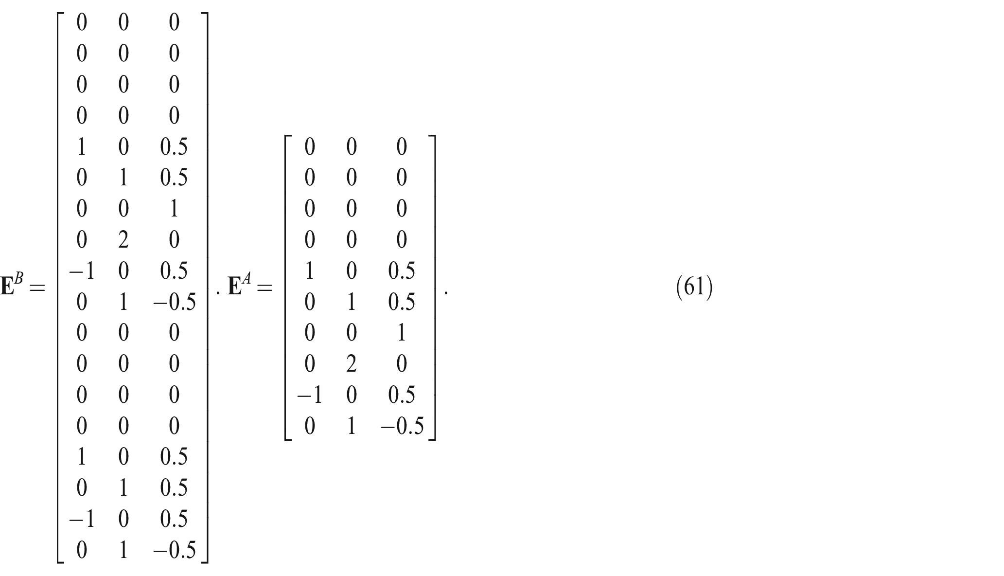
Considering the case of a square lattice as illustrated in Figure 2(a), and the related unit cell A, the kinematic and equilibrium formulation is expressed as:

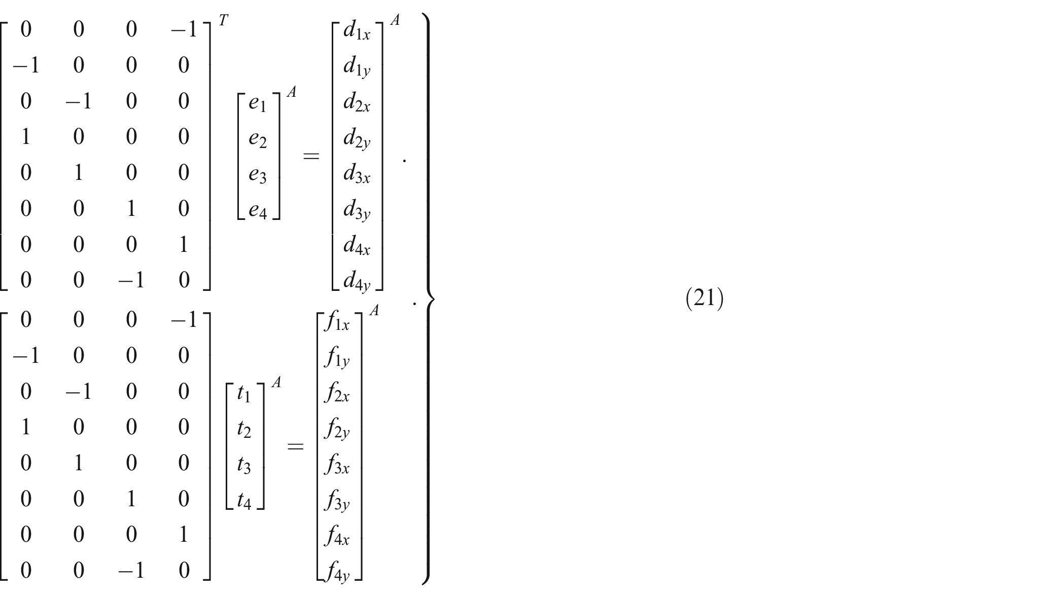
\begin{matrix} {[\begin{matrix} 0 & 0 & 0 & - 1 \\ - 1 & 0 & 0 & 0 \\ 0 & - 1 & 0 & 0 \\ 1 & 0 & 0 & 0 \\ 0 & 1 & 0 & 0 \\ 0 & 0 & 1 & 0 \\ 0 & 0 & 0 & 1 \\ 0 & 0 & - 1 & 0 \end{matrix}]}^{T} {[\begin{matrix} e_{1} \\ e_{2} \\ e_{3} \\ e_{4} \end{matrix}]}^{A} = {[\begin{matrix} d_{1 x} \\ d_{1 y} \\ d_{2 x} \\ d_{2 y} \\ d_{3 x} \\ d_{3 y} \\ d_{4 x} \\ d_{4 y} \end{matrix}]}^{A} . \\ [\begin{matrix} 0 & 0 & 0 & - 1 \\ - 1 & 0 & 0 & 0 \\ 0 & - 1 & 0 & 0 \\ 1 & 0 & 0 & 0 \\ 0 & 1 & 0 & 0 \\ 0 & 0 & 1 & 0 \\ 0 & 0 & 0 & 1 \\ 0 & 0 & - 1 & 0 \end{matrix}] {[\begin{matrix} t_{1} \\ t_{2} \\ t_{3} \\ t_{4} \end{matrix}]}^{A} = {[\begin{matrix} f_{1 x} \\ f_{1 y} \\ f_{2 x} \\ f_{2 y} \\ f_{3 x} \\ f_{3 y} \\ f_{4 x} \\ f_{4 y} \end{matrix}]}^{A} \end{matrix} .}

(21)

The kinematic and equilibrium formulation for unit cell B is as follows:

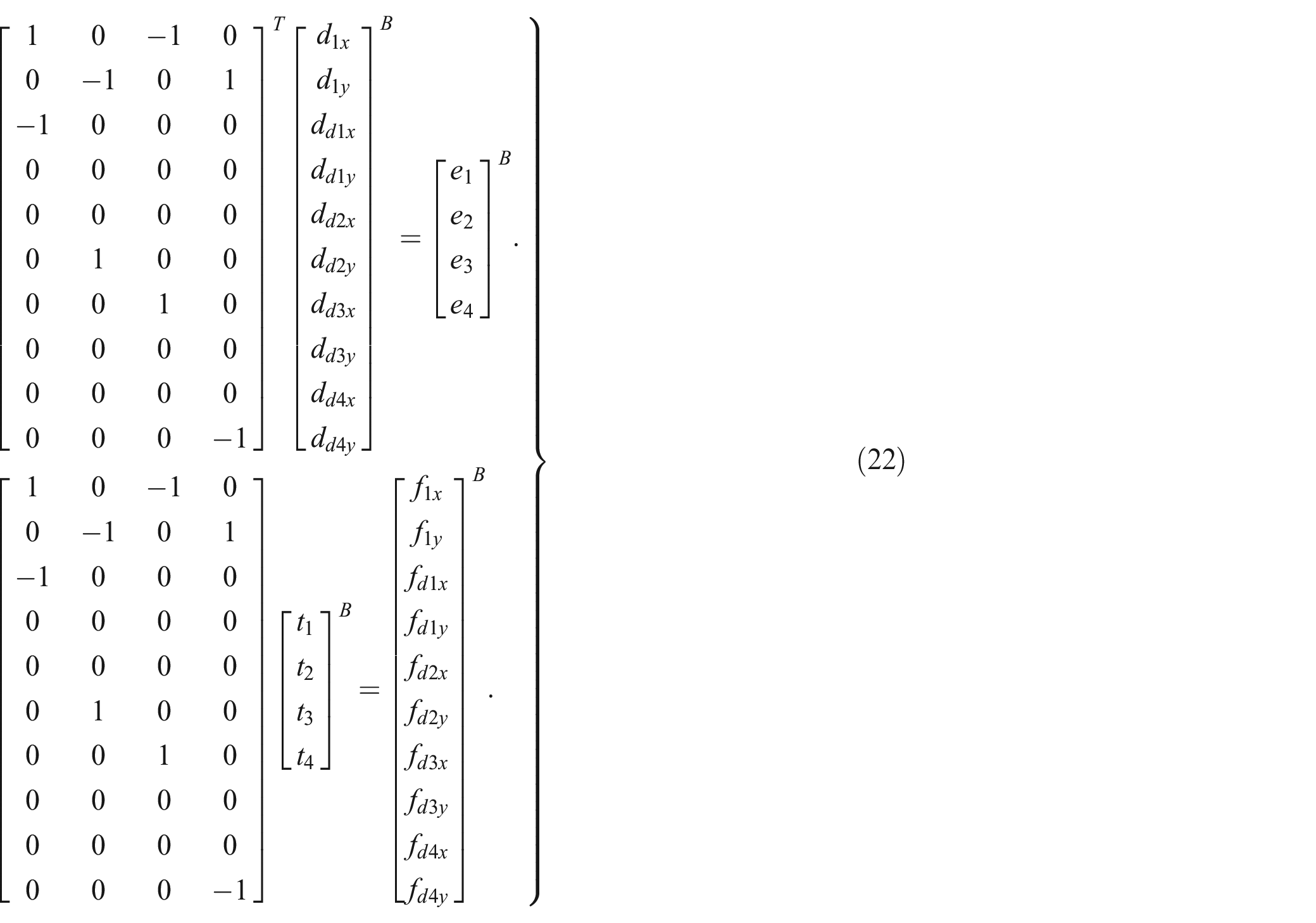
\begin{matrix} {[\begin{matrix} 1 & 0 & - 1 & 0 \\ 0 & - 1 & 0 & 1 \\ - 1 & 0 & 0 & 0 \\ 0 & 0 & 0 & 0 \\ 0 & 0 & 0 & 0 \\ 0 & 1 & 0 & 0 \\ 0 & 0 & 1 & 0 \\ 0 & 0 & 0 & 0 \\ 0 & 0 & 0 & 0 \\ 0 & 0 & 0 & - 1 \end{matrix}]}^{T} {[\begin{matrix} d_{1 x} \\ d_{1 y} \\ d_{d 1 x} \\ d_{d 1 y} \\ d_{d 2 x} \\ d_{d 2 y} \\ d_{d 3 x} \\ d_{d 3 y} \\ d_{d 4 x} \\ d_{d 4 y} \end{matrix}]}^{B} = {[\begin{matrix} e_{1} \\ e_{2} \\ e_{3} \\ e_{4} \end{matrix}]}^{B} . \\ [\begin{matrix} 1 & 0 & - 1 & 0 \\ 0 & - 1 & 0 & 1 \\ - 1 & 0 & 0 & 0 \\ 0 & 0 & 0 & 0 \\ 0 & 0 & 0 & 0 \\ 0 & 1 & 0 & 0 \\ 0 & 0 & 1 & 0 \\ 0 & 0 & 0 & 0 \\ 0 & 0 & 0 & 0 \\ 0 & 0 & 0 & - 1 \end{matrix}] {[\begin{matrix} t_{1} \\ t_{2} \\ t_{3} \\ t_{4} \end{matrix}]}^{B} = {[\begin{matrix} f_{1 x} \\ f_{1 y} \\ f_{d 1 x} \\ f_{d 1 y} \\ f_{d 2 x} \\ f_{d 2 y} \\ f_{d 3 x} \\ f_{d 3 y} \\ f_{d 4 x} \\ f_{d 4 y} \end{matrix}]}^{B} . \end{matrix}}

(22)

The removal of all DOFs connected to respective dummy nodes is the subsequent second stage. In Equation (22), the dotted rectangles encircle the modes connected to the dummy nodes in equilibrium and the kinematic systems. As a result, Equation (22) can be expressed as:

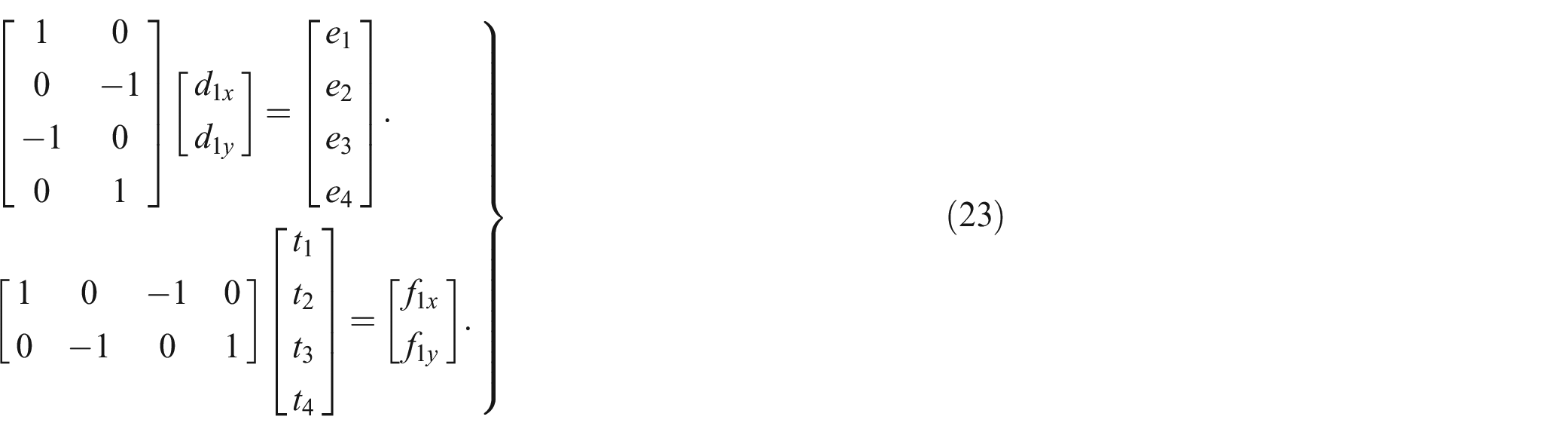
\begin{matrix} [\begin{matrix} 1 & 0 \\ 0 & - 1 \\ - 1 & 0 \\ 0 & 1 \end{matrix}] [\begin{matrix} d_{1 x} \\ d_{1 y} \end{matrix}] = [\begin{matrix} e_{1} \\ e_{2} \\ e_{3} \\ e_{4} \end{matrix}] . \\ [\begin{matrix} 1 & 0 & - 1 & 0 \\ 0 & - 1 & 0 & 1 \end{matrix}] [\begin{matrix} t_{1} \\ t_{2} \\ t_{3} \\ t_{4} \end{matrix}] = [\begin{matrix} f_{1 x} \\ f_{1 y} \end{matrix}] . \end{matrix}}

(23)

Considering the unit cell B, the kinematic and the equilibrium systems, as depicted in Figure 2(d), are represented by Equation (23). Bloch’s theorem definition and the dependence relations of the bar and the node bases are then utilized to establish the irreducible forms of the matrix systems in Equation (23). The IBZ related to the reciprocal lattice can be used to predict the lattice behavior at respective wave numbers based on the definition of the wave functions of the abovementioned irreducible lattice forms.

4.2. Derivation of the Cauchy–Born kinematic boundary condition: Homogenization of the mechanical properties of the lattice microstructure

In the process of kinematic system analysis for a given lattice structure, the kinematic boundary condition of the CBH is applied to the kinematic system of lattice structures at wave number $ω = (0, 0)$ . The objective is to derive an explicit expression of the microscopic element deformations in terms of a macroscopic strain field applied to the lattice structure [2]. This procedure is vital in deriving the lattice properties such as strength and effective stiffness.

A structure with $b$ components linked between $j$ nodes exhibits the following kinematic system:

B d = e .

(24)

where $B \in R^{b \times nj}$ is a Jacobian matrix (given that the case is 2D). The matrix entries correspond to the direction cosines used to obtain the vector representing the values of the element deformations $e \in R^{b}$ from those of the nodal displacements $d \in R^{nj}$ [46,47].

The Cauchy–Born boundary kinematic boundary condition [2] is expressed as:

d = T_{d} \tilde{d} + E \bar{ε} .

(25)

where $d \in R^{nj}$ is the vector of nodal displacements of the unit cell with $\tilde{d} \in R^{nJ}$ being the nodal displacement vector in the irreducible form. Here, $J$ is the number of independent nodes, whereas $E \in R^{nj \times 3}$ is the transformation matrix from the macroscopic strain field vector space $\bar{ε} \in R^{3}$ to the nodal displacement vector space $d \in R^{nj}$ . Also, $T_{d} \in R^{nj \times nJ}$ is the transformation matrix from the irreducible form of the nodal displacement vector space to the total nodal displacement vector space.

Based on the theory of Cauchy–Born, the kinematic boundary condition for a unit cell with its enclosing envelope coinciding with the constituent elements is derived using DNR and then applied to its kinematic system. This step is completed through the following elimination scheme:

1. At the sites where the cell elements coincide with the enclosing envelope and extend across multiple unit cells, hypothetical dummy nodes are inserted. As reported in Section 4.1, these dummy nodes are used to create the equilibrium and kinematic matrices related to the unit cell finite microstructure.

2. The dependency of node sets to differentiate between the independent and dependent set of nodes is identified by utilizing Equation (3) on the node bases group, which also incorporates the dummy nodes for the unit cell illustrated in Figure 2(e) and indicated in Table 1.

3. By creating the matrices $E$ and $T_{d}$ and applying them to the unit cell kinematic system created in Step 1, the dependence relations produced in Step 2 can now be utilized for kinematic boundary formulation based on the Cauchy–Born condition. Consequently, the following relation can be derived:

\underset{1}{\underset{︸}{B \bar{E \tilde{\bar{ε}}}}} + \underset{2}{\underset{︸}{B \bar{T_{d} \tilde{d}}}} = e .

(26)

under the condition that $BE \bar{ε} \in R^{\dim (e) \times 3}$ and ${BT}_{d} \tilde{d} \in R^{\dim (e) \times \dim (\tilde{d})}$ .

The DOFs related to the dummy nodes are incorporated in the second term on the left side of Equation (26).

4. From Equation (26), the second term on the left side denotes hypothetical dummy nodes’ DOF and is removed from the matrix system, similar to the procedure explained by Section 4.1.1.

It should be noted that the second term in Equation (26), which accounts only for the dependencies of the real nodes, is similar to the lattice’s kinematic system in its reduced form, obtained by applying Bloch’s wave reduction at wave number $ω = (0, 0)$ after the DOFs linked to the dummy nodes have been removed. The element dependency reduction [2] is a further step in determining the microscopic element deformations as an expression of the macroscopic strain field. Details of this analysis can be found by Elsayed and Pasini [2].

The matrix $E^{B} \in R^{10 \times 3}$ for the unit cell B illustrated in Figure 2(e) can be derived as:

E^{B} = [\begin{matrix} 0 & 0 & 0 \\ 0 & 0 & 0 \\ 0 & 0 & 0 \\ 0 & 0 & 0 \\ 0 & 0 & 0 \\ 0 & 0 & 0 \\ 1 & 0 & 0 \\ 0 & 0 & 0.5 \\ 0 & 0 & - 0.5 \\ 0 & - 1 & 0 \end{matrix}] .

(27)

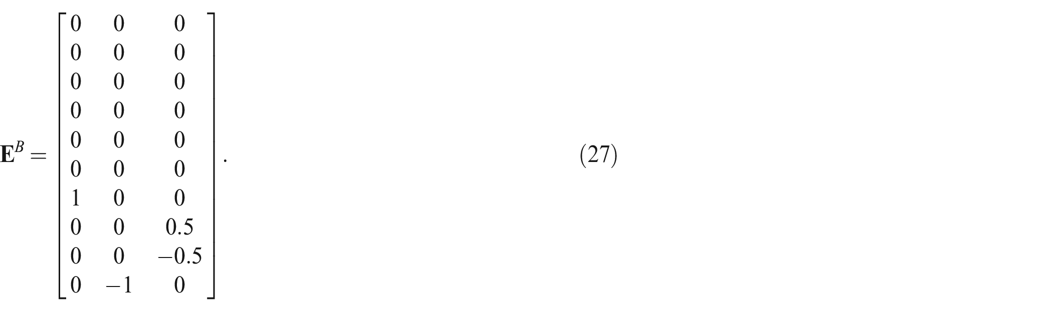
The first term on the left-hand side of Equation (26) is generated when the kinematic matrix of a unit cell, as indicated in Equation (22), including the dummy nodes, is multiplied by the matrix E stated above in Equation (27):

B^{B} E^{B} \bar{ε} = [\begin{matrix} 0 & 0 & 0 \\ 0 & 0 & 0 \\ 1 & 0 & 0 \\ 0 & 1 & 0 \end{matrix}] ⌈ \begin{matrix} {\bar{ε}}_{xx} \\ {\bar{ε}}_{yy} \\ {\bar{ε}}_{xy} \end{matrix} ⌉ .

(28)

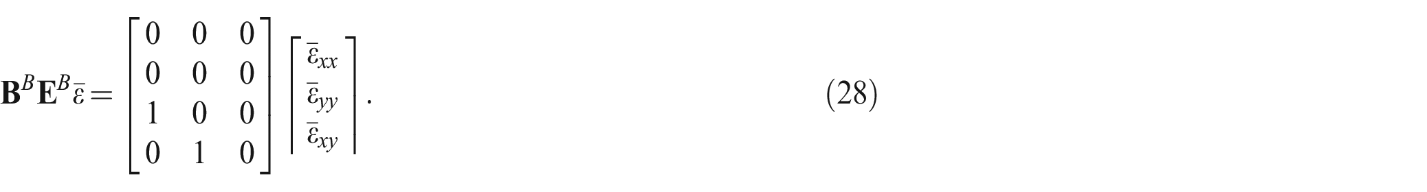
Table 2 shows that there is no dependency relation for the real nodes of cell B, that is, the system produced by the nodal wave functions is similar to the kinematic system given in Equation (23) for the application of the wave reduction technique based on Bloch’s theorem. Accordingly, the final form of Equation (26) is as follows:

[\begin{matrix} 1 & 0 \\ 0 & - 1 \\ - 1 & 0 \\ 0 & 1 \end{matrix}] {⌈ \begin{matrix} d_{1 x} \\ d_{1 y} \end{matrix} ⌉}^{B} + [\begin{matrix} 0 & 0 & 0 \\ 0 & 0 & 0 \\ 1 & 0 & 0 \\ 0 & 1 & 0 \end{matrix}] ⌈ \begin{matrix} {\bar{ε}}_{x x} \\ {\bar{ε}}_{y y} \\ {\bar{ε}}_{x y} \end{matrix} ⌉ = {⌈ \begin{matrix} e_{1} \\ e_{2} \\ e_{3} \\ e_{4} \end{matrix} ⌉}^{B} .

(29)

For unit cell A, the matrix $E^{A} \in R^{8 \times 3}$ is formulated as follows:

E^{A} = [\begin{matrix} 0 & 0 & 0 \\ 0 & 0 & 0 \\ 0 & 0 & 0.5 \\ 0 & 1 & 0 \\ 1 & 0 & 0.5 \\ 0 & 1 & 0.5 \\ 1 & 0 & 0 \\ 0 & 0 & 0.5 \end{matrix}] .

(30)

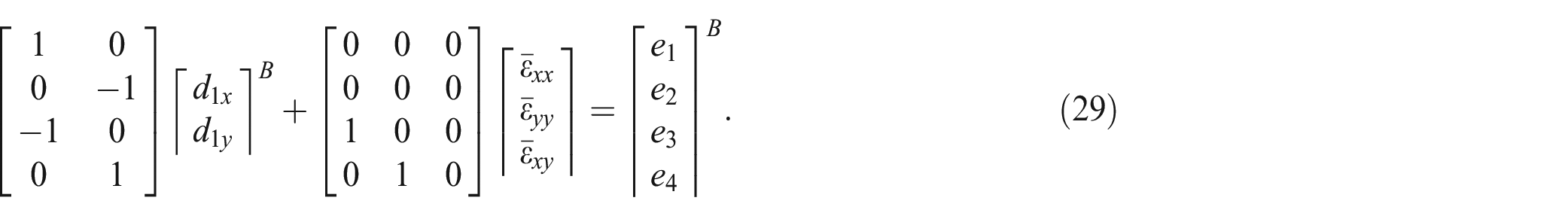
Furthermore, Equation (26) can be formulated as follows:

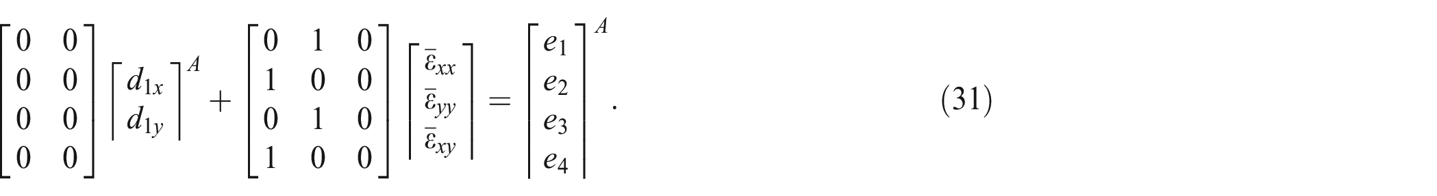
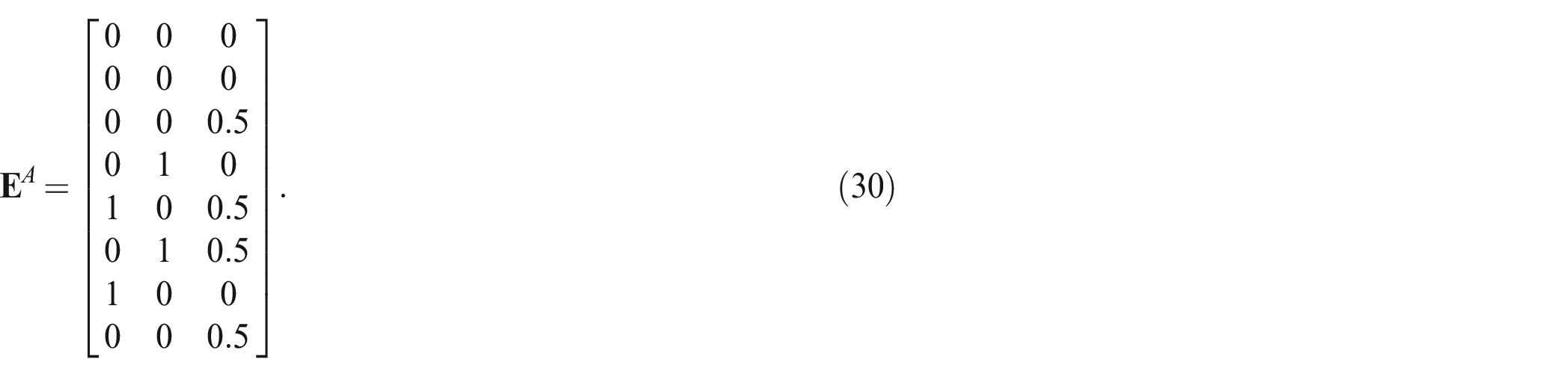
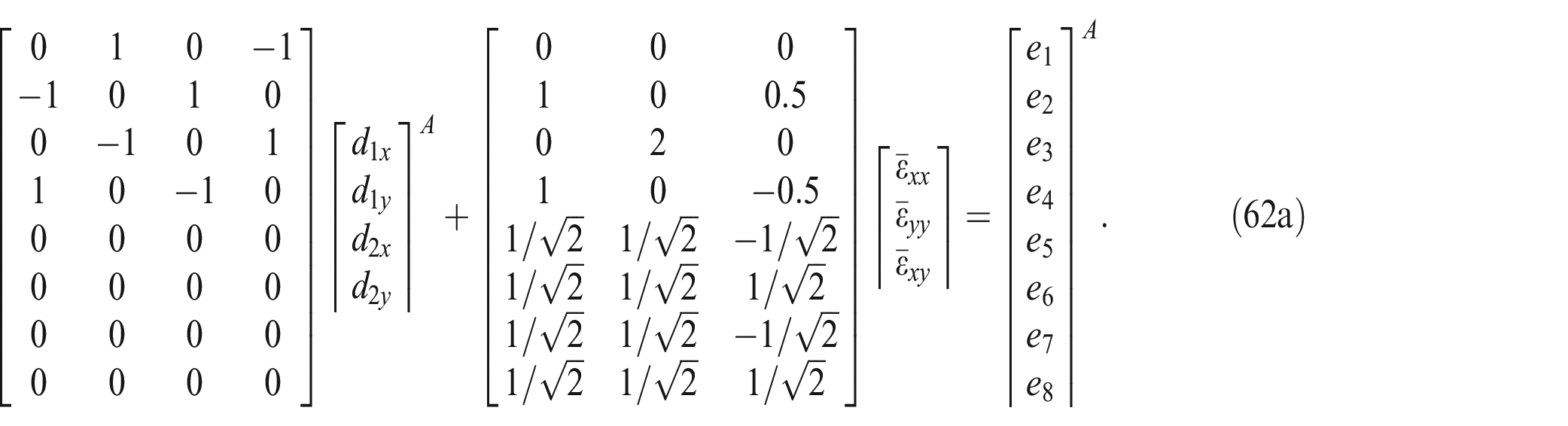
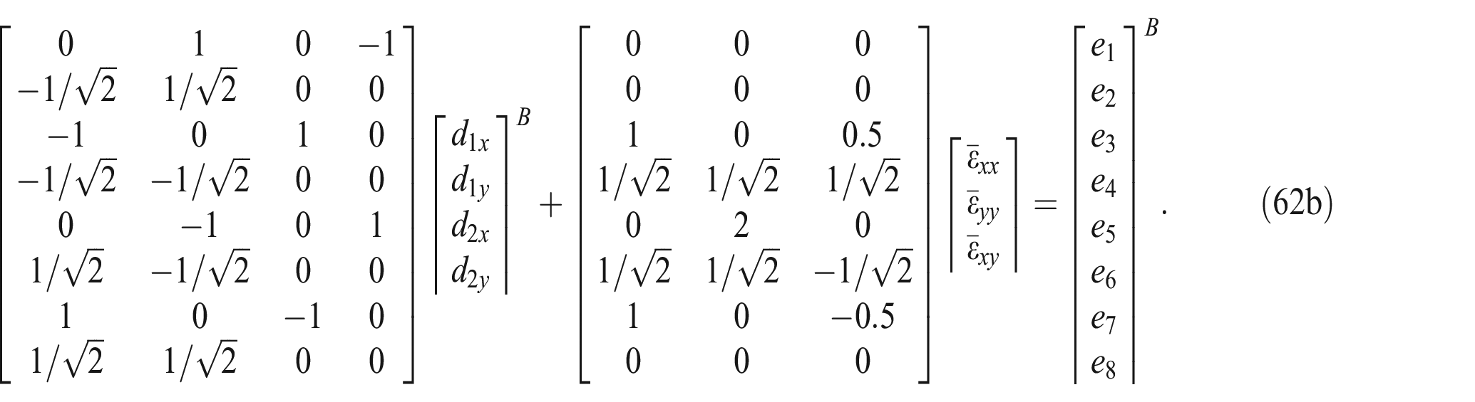
[\begin{matrix} 0 & 0 \\ 0 & 0 \\ 0 & 0 \\ 0 & 0 \end{matrix}] {⌈ \begin{matrix} d_{1 x} \\ d_{1 y} \end{matrix} ⌉}^{A} + [\begin{matrix} 0 & 1 & 0 \\ 1 & 0 & 0 \\ 0 & 1 & 0 \\ 1 & 0 & 0 \end{matrix}] ⌈ \begin{matrix} {\bar{ε}}_{xx} \\ {\bar{ε}}_{yy} \\ {\bar{ε}}_{xy} \end{matrix} ⌉ = {⌈ \begin{matrix} e_{1} \\ e_{2} \\ e_{3} \\ e_{4} \end{matrix} ⌉}^{A} .

(31)

The matrix systems of Equations (29) and (31) utilize the macroscopic strain field variables to characterize an explicit derivation of the microscopic cell element deformations. This analysis results in the following:

{⌈ \begin{matrix} e_{1} \\ e_{2} \\ e_{3} \\ e_{4} \end{matrix} ⌉}^{A} = [\begin{matrix} 0 & 1 & 0 \\ 1 & 0 & 0 \\ 0 & 1 & 0 \\ 1 & 0 & 0 \end{matrix}] ⌈ \begin{matrix} {\bar{ε}}_{xx} \\ {\bar{ε}}_{yy} \\ {\bar{ε}}_{xy} \end{matrix} ⌉ .

(32a)

{⌈ \begin{matrix} e_{1} \\ e_{2} \\ e_{3} \\ e_{4} \end{matrix} ⌉}^{B} = [\begin{matrix} 0.5 & 0 & 0 \\ 0 & 0.5 & 0 \\ 0.5 & 0 & 0 \\ 0 & 0.5 & 0 \end{matrix}] ⌈ \begin{matrix} {\bar{ε}}_{xx} \\ {\bar{ε}}_{yy} \\ {\bar{ε}}_{xy} \end{matrix} ⌉ .

(32b)

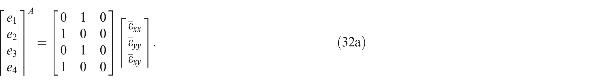
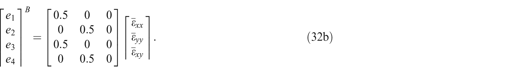
The element deformations concerning cell A and cell B are, respectively, described by Equation (32a) and Equation (32b) and then provide a pathway to investigating the macroscopic stiffness of the lattice:

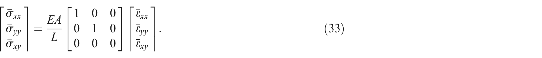
⌈ \begin{matrix} {\bar{σ}}_{xx} \\ {\bar{σ}}_{yy} \\ {\bar{σ}}_{xy} \end{matrix} ⌉ = \frac{EA}{L} [\begin{matrix} 1 & 0 & 0 \\ 0 & 1 & 0 \\ 0 & 0 & 0 \end{matrix}] ⌈ \begin{matrix} {\bar{ε}}_{xx} \\ {\bar{ε}}_{yy} \\ {\bar{ε}}_{xy} \end{matrix} ⌉ .

(33)

where $E$ is Young’s modulus of the base material of the lattice structure. Here, $L$ is the length, and $A$ is the cross-sectional area of the cell element at the microscale level.

4.3. Elimination scheme—proof and validation

In the three-unit cell configuration of the lattice structure depicted in Figure 4, two constituent elements $m$ and $n$ can have unit vectors in their respective directions, such as:

{\hat{n}}_{m} = \frac{j_{i} - j_{k}}{L_{m 1}} = \frac{j_{p} - j_{i}}{L_{m 2}} = \frac{j_{p} - j_{k}}{L_{m}} .

(34)

{\hat{n}}_{n} = \frac{j_{j} - j_{q}}{L_{n 1}} = \frac{j_{l} - j_{j}}{L_{n 2}} = \frac{j_{l} - j_{q}}{L_{n}} .

(35)

4.3.1. Equilibrium Analysis

For a structure with $j$ nodes and $b$ interconnecting elements, the static equilibrium is evaluated by:

A t = f .

(36)

where A is the Jacobian matrix denoted by $A \in R^{nj \times b}$ with n = 2 in a 2D setting, comprising direction cosines that facilitate the establishment of the nodal forces vector. Here, $f \in R^{nj}$ from tension forces at the level of the structural elements [46,47].

Applying static equilibrium condition for forces experienced at node $k$ and node $i$ , for the segment $m 1$ of unit cell element $m$ subjected to tension force $t_{m}$ :

⌈ \begin{matrix} - {\hat{n}}_{m} \\ {\hat{n}}_{m} \end{matrix} ⌉ t_{m} = ⌈ \begin{matrix} f_{k} \\ f_{i} \end{matrix} ⌉ .

(37)

Similarly, the static equilibrium condition for forces experienced at node $i$ and node $p$ , for the segment $m 2$ of unit cell element subjected to tension force $t_{m}$ :

⌈ \begin{matrix} - {\hat{n}}_{m} \\ {\hat{n}}_{m} \end{matrix} ⌉ t_{m} = ⌈ \begin{matrix} f_{i} \\ f_{p} \end{matrix} ⌉ .

(38)

A single matrix can be formed from the combination of Equations (37) and (38):

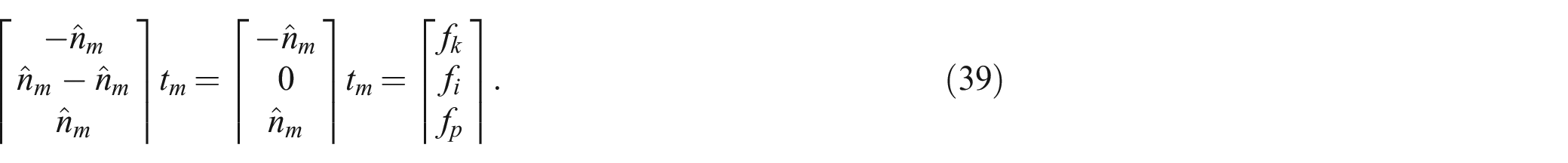
⌈ \begin{matrix} - {\hat{n}}_{m} \\ {\hat{n}}_{m} - {\hat{n}}_{m} \\ {\hat{n}}_{m} \end{matrix} ⌉ t_{m} = ⌈ \begin{matrix} - {\hat{n}}_{m} \\ 0 \\ {\hat{n}}_{m} \end{matrix} ⌉ t_{m} = ⌈ \begin{matrix} f_{k} \\ f_{i} \\ f_{p} \end{matrix} ⌉ .

(39)

Since the coefficients associated with the dummy node, $i$ , are specified as zero in Equation (39), the node may be removed from the matrix system, which yields:

⌈ \begin{matrix} - {\hat{n}}_{m} \\ {\hat{n}}_{m} \end{matrix} ⌉ t_{m} = ⌈ \begin{matrix} f_{k} \\ f_{p} \end{matrix} ⌉ .

(40)

For element $n$ , an identical approach may be defined to describe the equilibrium between the elemental tension forces $t_{n}$ , expressed at respective nodes $q$ , $j$ , and $l$ in Equations (41) and (42).

⌈ \begin{matrix} - {\hat{n}}_{n} \\ {\hat{n}}_{n} \end{matrix} ⌉ t_{n} = ⌈ \begin{matrix} f_{q} \\ f_{j} \end{matrix} ⌉ .

(41)

⌈ \begin{matrix} - {\hat{n}}_{n} \\ {\hat{n}}_{n} \end{matrix} ⌉ t_{n} = ⌈ \begin{matrix} f_{j} \\ f_{l} \end{matrix} ⌉ .

(42)

A single matrix can be formed from the combination of Equations (41) and (42):

⌈ \begin{matrix} - {\hat{n}}_{n} \\ {\hat{n}}_{n} \end{matrix} ⌉ t_{n} = ⌈ \begin{matrix} f_{q} \\ f_{l} \end{matrix} ⌉ .

(43)

In the next step, element segments $m 1$ and $n 2$ of elements $m$ and $n$ , respectively, lying within the second unit cell envelope, are evaluated for their kinematic compatibility. Utilizing the DNR at wave number $ω = (0, 0)$ , the static relations of elements $m$ and $n$ and dummy nodes $i$ and $j$ can be established as:

{\hat{n}}_{m} = {\hat{n}}_{n} .

t_{m} = - t_{n} .

f_{i} = - f_{j} .

(44)

Now, the assembly of the equilibrium of element segment $m 1$ (Equation (37)) and element segment $n 2$ (Equation (42)) of elements $m$ and $n$ , respectively, can be combined into a single matrix as:

[\begin{matrix} - {\hat{n}}_{m} & 0 \\ {\hat{n}}_{m} & 0 \\ 0 & - {\hat{n}}_{n} \\ 0 & {\hat{n}}_{n} \end{matrix}] ⌈ \begin{matrix} t_{m} \\ t_{n} \end{matrix} ⌉ = ⌈ \begin{matrix} f_{k} \\ f_{i} \\ f_{j} \\ f_{l} \end{matrix} ⌉ .

(45)

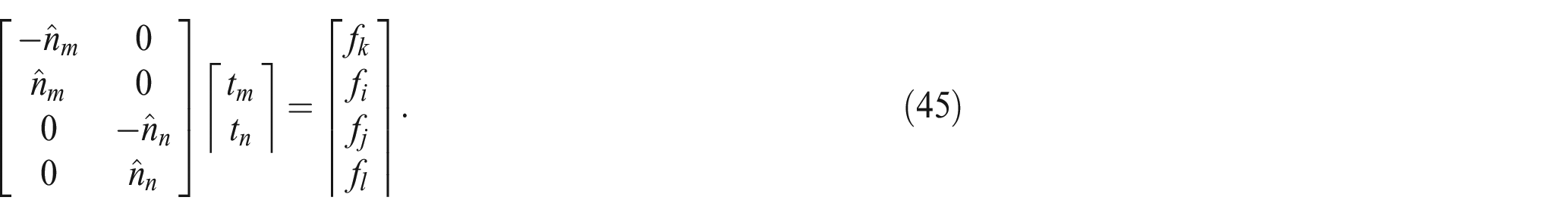
Considering results of Equation (44):

⌈ \begin{matrix} - {\hat{n}}_{m} \\ {\hat{n}}_{m} \\ {\hat{n}}_{n} \\ - {\hat{n}}_{n} \end{matrix} ⌉ ⌈ t_{m} ⌉ = {⌈ \begin{matrix} f_{k} \\ f_{i} \\ f_{j} \\ f_{l} \end{matrix} ⌉}_{t_{m} = - t_{n}} .

⌈ \begin{matrix} - {\hat{n}}_{m} \\ {\hat{n}}_{m} - {\hat{n}}_{n} \\ - {\hat{n}}_{n} \end{matrix} ⌉ ⌈ t_{m} ⌉ = {⌈ \begin{matrix} f_{k} \\ f_{i} \\ f_{l} \end{matrix} ⌉}_{f_{i} = - f_{j}} .

⌈ \begin{matrix} - {\hat{n}}_{m} \\ 0 \\ - {\hat{n}}_{m} \end{matrix} ⌉ ⌈ t_{m} ⌉ = {⌈ \begin{matrix} f_{k} \\ f_{i} \\ f_{l} \end{matrix} ⌉}_{{\hat{n}}_{m} = {\hat{n}}_{n}} .

(46)

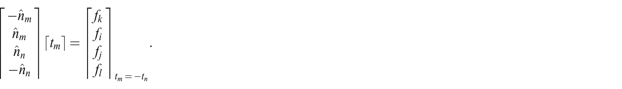
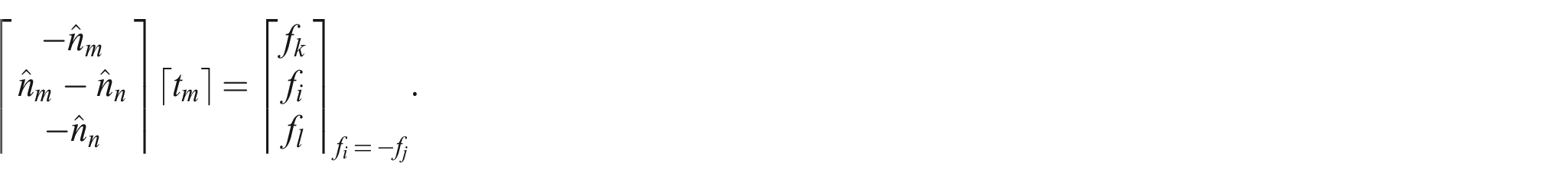
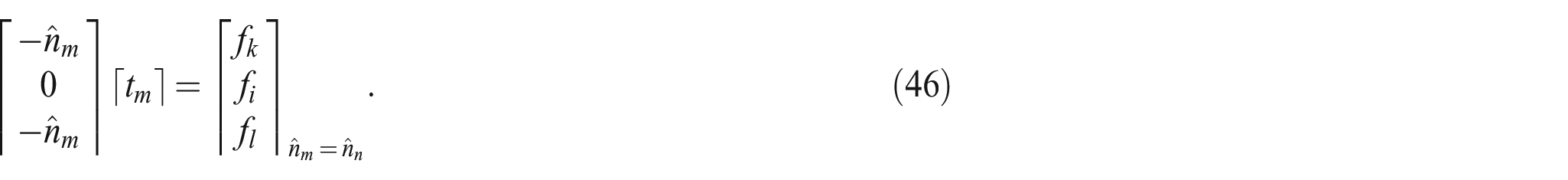
The subscript is utilized to indicate the applied condition. Ultimately, the matrix system represented by Equation (46) is simplified to:

⌈ \begin{matrix} - {\hat{n}}_{m} \\ - {\hat{n}}_{m} \end{matrix} ⌉ t_{m} = ⌈ \begin{matrix} - {\hat{n}}_{m} & 0 \\ 0 & {\hat{n}}_{m} \end{matrix} ⌉ ⌈ \begin{matrix} t_{m} \\ t_{n} \end{matrix} ⌉ = ⌈ \begin{matrix} f_{k} \\ f_{l} \end{matrix} ⌉ .

(47)

For the dummy nodes $i$ and $j$ , this in effect removes the associated DOFs from the assembly. It is noteworthy that the matrix system derived from the above Equation (47) is similar to the outcomes obtained from Equations (40) and (43).

4.3.2. Kinematic Analysis

The kinematic compatibility condition between the deformation $e_{m 1}$ of a portion of segment $m 1$ of element $m$ and displacements of the node $k$ and node $i$ can be expressed as follows:

[\begin{matrix} {\hat{n}}_{m} & - {\hat{n}}_{m} \end{matrix}] ⌈ \begin{matrix} d_{k} \\ d_{i} \end{matrix} ⌉ = e_{m 1}

(48)

Similarly, the kinematic compatibility condition between the deformation $e_{m 2}$ of a portion of segment $m 2$ of element $m$ and displacements of node $i$ and node $j$ can be expressed as follows:

[\begin{matrix} {\hat{n}}_{m} & - {\hat{n}}_{m} \end{matrix}] ⌈ \begin{matrix} d_{i} \\ d_{p} \end{matrix} ⌉ = e_{m 2} .

(49)

Combining Equations (48) and (49) yields:

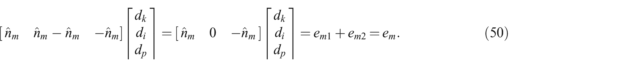
[\begin{matrix} {\hat{n}}_{m} & {\hat{n}}_{m} - {\hat{n}}_{m} & - {\hat{n}}_{m} \end{matrix}] ⌈ \begin{matrix} d_{k} \\ d_{i} \\ d_{p} \end{matrix} ⌉ = [\begin{matrix} {\hat{n}}_{m} & 0 & - {\hat{n}}_{m} \end{matrix}] ⌈ \begin{matrix} d_{k} \\ d_{i} \\ d_{p} \end{matrix} ⌉ = e_{m 1} + e_{m 2} = e_{m} .

(50)

Equation (50) indicates that the dummy node $i$ coefficients are assigned a value of zero. This facilitates the removal of the node with respect to the assembly of the matrix system, leading to the following outcome:

[\begin{matrix} {\hat{n}}_{m} & - {\hat{n}}_{m} \end{matrix}] ⌈ \begin{matrix} d_{k} \\ d_{p} \end{matrix} ⌉ = e_{m} .

(51)

A similar procedure can be extended to element $n$ . The kinematic compatibility between the element deformation $e_{n}$ and the displacement of the node $q$ , node $j$ , and node $l$ is indicated in Equations (52) and (53):

[\begin{matrix} {\hat{n}}_{n} & - {\hat{n}}_{n} \end{matrix}] ⌈ \begin{matrix} d_{q} \\ d_{j} \end{matrix} ⌉ = e_{n 1} .

(52)

[\begin{matrix} {\hat{n}}_{n} & - {\hat{n}}_{n} \end{matrix}] ⌈ \begin{matrix} d_{j} \\ d_{l} \end{matrix} ⌉ = e_{n 2} .

(53)

Combining Equations (52) and (53) yields:

[\begin{matrix} {\hat{n}}_{n} & - {\hat{n}}_{n} \end{matrix}] ⌈ \begin{matrix} d_{q} \\ d_{l} \end{matrix} ⌉ = e_{n} .

(54)

In the next step, element segments $m 1$ and $n 2$ of elements $m$ and $n$ , enclosed by the second unit cell envelope, are evaluated for their kinematic compatibility.

Utilizing the DNR at wave number $ω = (0, 0)$ , the kinematic relations of elements $m$ and $n$ and dummy nodes $i$ and . can be established as:

e_{m 1} + e_{n 2} = e_{m 2} + e_{n 1} = e_{m} = e_{n} and d_{i} = d_{j} .

(55)

Now, the assembly of the kinematic compatibilities of element segment $m 1$ (Equation (48)) and element segment $n 2$ (Equation (53)) of elements $m$ and $n$ , respectively, can be combined into a single matrix as:

[\begin{matrix} {\hat{n}}_{m} & - {\hat{n}}_{m} & {\hat{n}}_{n} & - {\hat{n}}_{n} \end{matrix}] ⌈ \begin{matrix} d_{k} \\ d_{i} \\ d_{j} \\ d_{l} \end{matrix} ⌉ = e_{m 1} + e_{n 2} .

(56)

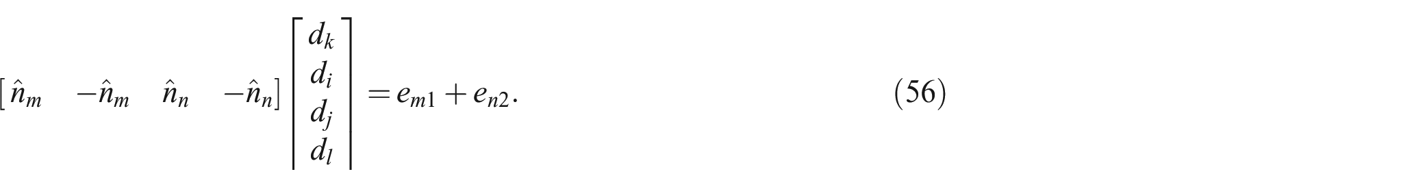
Considering results of Equation (55):

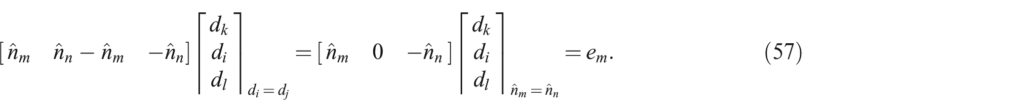
[\begin{matrix} {\hat{n}}_{m} & {\hat{n}}_{n} - {\hat{n}}_{m} & - {\hat{n}}_{n} \end{matrix}] {⌈ \begin{matrix} d_{k} \\ d_{i} \\ d_{l} \end{matrix} ⌉}_{d_{i} = d_{j}} = [\begin{matrix} {\hat{n}}_{m} & 0 & - {\hat{n}}_{n} \end{matrix}] {⌈ \begin{matrix} d_{k} \\ d_{i} \\ d_{l} \end{matrix} ⌉}_{{\hat{n}}_{m} = {\hat{n}}_{n}} = e_{m} .

(57)

where the associated subscript represents the applied condition. Ultimately, the matrix system represented by Equation (57) is simplified to:

[\begin{matrix} {\hat{n}}_{m} & - {\hat{n}}_{n} \end{matrix}] ⌈ \begin{matrix} d_{k} \\ d_{l} \end{matrix} ⌉ = e_{m} .

(58)

For the dummy node $si$ and $j$ , this, in effect, removes the associated DOFs from the assembly of the matrix system.

The preceding analysis indicates that in lattice structures, a substantial improvement is recorded for its matrix computation by adopting the proposed DNR technique. However, it is to be considered that the given methodology has been developed for a pin-jointed lattice structure, and any scenario where the DOFs linked with the dummy nodes fail to get eliminated would lead to unreliable outcomes.

5. Applications

5.1. Example 1

The lattice structure illustrated in Figure 5(a) is produced by utilizing unit cells A and B. This section outlines the process of evaluating the stiffness properties of the generated lattice structure. The unit cell depicted in Figure 5(c), denoted as A, comprises eight cell elements within the boundary of the cell envelope. The unit cell depicted in Figure 5(e), denoted as B, also comprises eight cell elements. Among these, four elements are within the boundary of the cell envelope, whereas the four elements are beyond the unit cell and coincide with the envelope. 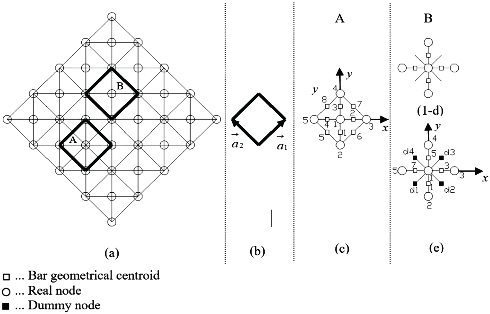The introduction of four dummy nodes, namely $d 1$ , $d 2$ , $d 3,$ and $d 4$ occurs within unit cell B. These nodes are situated at the points at which the cell elements coincide with the envelope and span across the adjacent cells.

Figure 5.

(a) lattice structure, (b) cell envelope, (c) unit cell B, (d) unit cell A without dummy nodes, and (e) unit cell A with dummy nodes [32].

This case study aims to showcase the precision of the developed elimination method and DNR, as two-unit cells, A and B, are utilized for the characterization process. The same process can be simple for most cases, such as unit cell A, and can be done based on literature results. In contrast, cases such as that of unit cell B necessitate the utilization of the DNR methodology. The proposed method has been demonstrated to be accurate, as both approaches yield similar lattice properties.

The first step in the characterization procedure is to specify the bases groups of the node, dummy node, and bar of unit cells A and B, respectively.

$G_{N}^{A} = {(0, 0), (0, - 1), (1, 0), (0, 1), (- 1, 0)}$ .

$G_{D}^{A} = Ø$ .

$G_{B}^{A} = {(0, - 0.5), (0.5, 0), (0, 0.5), (- 0.5, 0), (- 0.5, - 0.5), (0.5, - 0.5), (0.5, 0.5), (- 0.5, 0.5)}$ .

$G_{N}^{B} = {(0, 0), (0, - 1), (1, 0), (0, 1), (- 1, 0), (- 0.5, - 0.5), (0.5, - 0.5), (0.5, 0.5), (- 0.5, 0.5)}$ .

$G_{D}^{B} = {(- 0.5, - 0.5), (0.5, - 0.5), (0.5, 0.5), (- 0.5, 0.5)}$ .

$G_{B}^{B} = {(0, - 0.5), (0.5, - 0.5), (0.5, 0), (0.5, 0.5), (0, 0.5), (- 0.5, 0.5), (- 0.5, 0), (- 0.5, - 0.5)}$ .

The bases of the reciprocal lattice are as follows:

${\vec{b}}_{1} = (0.5, 0.5) .$

${\vec{b}}_{2} = (- 0.5, 0.5)$ .

With,

$j_{d 1} = b_{8} j_{d 1} = b_{8}$ .

$j_{d 2} = b_{2} j_{d 2} = b_{2}$ .

$j_{d 3} = b_{4} j_{d 3} = b_{4}$ .

$j_{d 4} = b_{6} j_{d 4} = b_{6}$ .

The formulation of the direct translational basis is as follows:

${\vec{a}}_{1} = (1, 1)$ .

${\vec{a}}_{2} = (- 1, 1)$ .

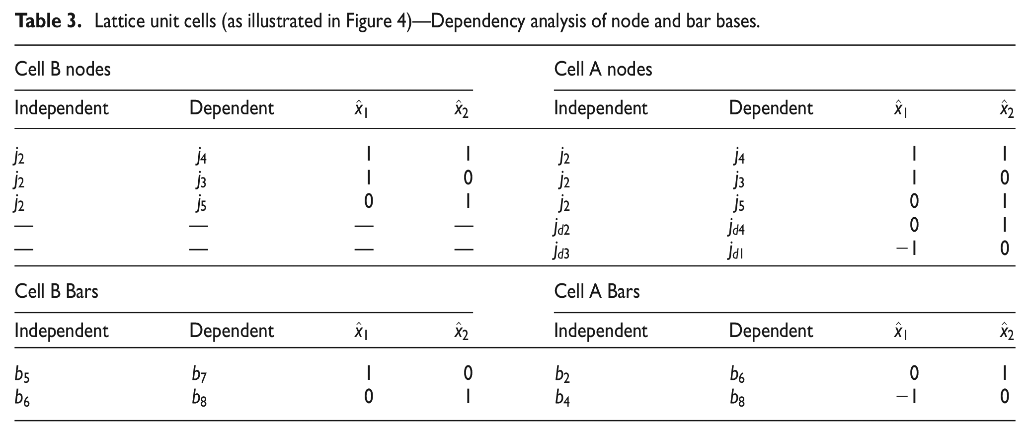
The dependency relations concerning the bar and node bases are listed in Table 3 and were determined using Equation (3).

Table 3.

Lattice unit cells (as illustrated in Figure 4)—Dependency analysis of node and bar bases.

Cell B nodes				Cell A nodes
Independent	Dependent	${\hat{x}}_{1}$	${\hat{x}}_{2}$	Independent	Dependent	${\hat{x}}_{1}$	${\hat{x}}_{2}$
$j_{2}$	$j_{4}$	1	1	$j_{2}$	$j_{4}$	1	1
$j_{2}$	$j_{3}$	1	0	$j_{2}$	$j_{3}$	1	0
$j_{2}$	$j_{5}$	0	1	$j_{2}$	$j_{5}$	0	1
—	—	—	—	$j_{d 2}$	$j_{d 4}$	0	1
—	—	—	—	$j_{d 3}$	$j_{d 1}$	−1	0
Cell B Bars				Cell A Bars
Independent	Dependent	${\hat{x}}_{1}$	${\hat{x}}_{2}$	Independent	Dependent	${\hat{x}}_{1}$	${\hat{x}}_{2}$
$b_{5}$	$b_{7}$	1	0	$b_{2}$	$b_{6}$	0	1
$b_{6}$	$b_{8}$	0	1	$b_{4}$	$b_{8}$	−1	0

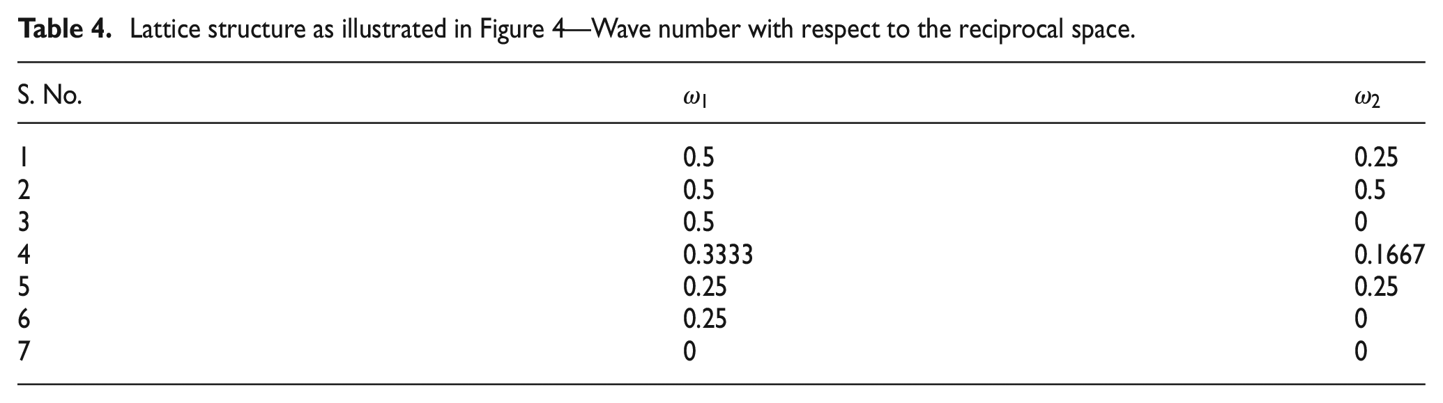
On the contrary, with respect to the lattice, the reciprocal space can be derived through the lattice reciprocal bases, and the IBZ, as illustrated in Figure 6, can be obtained through point group symmetry. Subsequently, as shown in Table 4, wave numbers can be derived, representing values at which the irreducible wave functions are analyzed through Bloch’s theorem.

Figure 6.

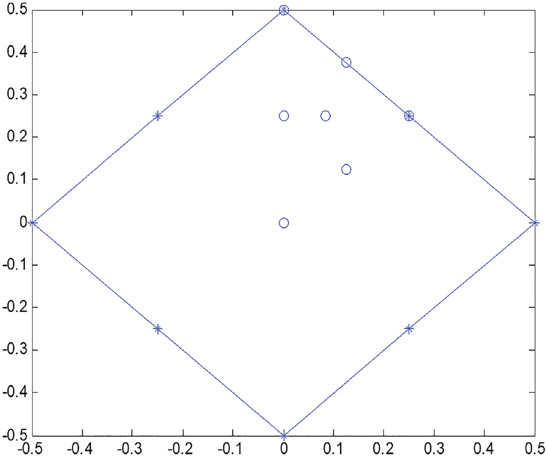
Lattice structure indicated in Figure 4(a)—First Brillouin zone and IBZ.

Table 4.

Lattice structure as illustrated in Figure 4—Wave number with respect to the reciprocal space.

S. No.	$ω_{1}$	$ω_{2}$
1	0.5	0.25
2	0.5	0.5
3	0.5	0
4	0.3333	0.1667
5	0.25	0.25
6	0.25	0
7	0	0

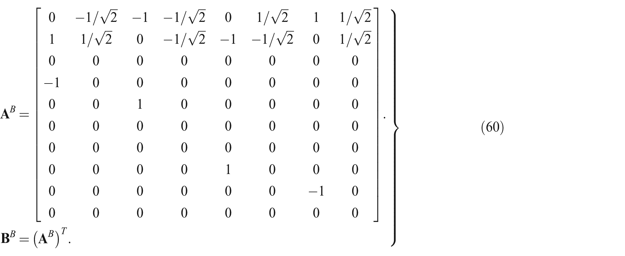
The kinematic and the equilibrium systems related to a unit cell’s finite structure can be obtained by using the bases groups defined earlier.

A^{A} = [\begin{matrix} 0 & - 1 & 1 & 0 & 0 & 0 & 0 & 0 \\ 1 & 0 & - 1 & 0 & 0 & 0 & 0 & 0 \\ 0 & 0 & 0 & 0 & 1 / \sqrt{2} & - 1 / \sqrt{2} & 0 & 0 \\ - 1 & 0 & 0 & 0 & - 1 / \sqrt{2} & 1 / \sqrt{2} & 0 & 0 \\ 0 & 1 & 0 & 0 & 0 & 1 / \sqrt{2} & 1 / \sqrt{2} & 0 \\ 0 & 0 & 0 & 0 & 0 & 1 / \sqrt{2} & - 1 / \sqrt{2} & 0 \\ 0 & 0 & 0 & 0 & 0 & 0 & - 1 / \sqrt{2} & 1 / \sqrt{2} \\ 0 & 0 & 1 & 0 & 0 & 0 & 1 / \sqrt{2} & 1 / \sqrt{2} \\ 0 & 0 & 0 & - 1 & - 1 / \sqrt{2} & 0 & 0 & - 1 / \sqrt{2} \\ 0 & 0 & 0 & 0 & 1 / \sqrt{2} & 0 & 0 & - 1 / \sqrt{2} \end{matrix}] . B^{A} = {(A^{A})}^{T} .

(59a)

A_{d}^{B} = [\begin{matrix} 0 & - 1 / \sqrt{2} & - 1 & - 1 / \sqrt{2} & 0 & 1 / \sqrt{2} & 1 & 1 / \sqrt{2} \\ 1 & 1 / \sqrt{2} & 0 & - 1 / \sqrt{2} & - 1 & - 1 / \sqrt{2} & 0 & 1 / \sqrt{2} \\ 0 & 0 & 0 & 0 & 0 & 0 & 0 & 0 \\ - 1 & 0 & 0 & 0 & 0 & 0 & 0 & 0 \\ 0 & 0 & 1 & 0 & 0 & 0 & 0 & 0 \\ 0 & 0 & 0 & 0 & 0 & 0 & 0 & 0 \\ 0 & 0 & 0 & 0 & 0 & 0 & 0 & 0 \\ 0 & 0 & 0 & 0 & 1 & 0 & 0 & 0 \\ 0 & 0 & 0 & 0 & 0 & 0 & - 1 & 0 \\ 0 & 0 & 0 & 0 & 0 & 0 & 0 & 0 \\ 0 & 0 & 0 & 0 & 0 & 0 & 0 & - 1 / \sqrt{2} \\ 0 & 0 & 0 & 0 & 0 & 0 & 0 & - 1 / \sqrt{2} \\ 0 & 1 / \sqrt{2} & 0 & 0 & 0 & 0 & 0 & 0 \\ 0 & - 1 / \sqrt{2} & 0 & 0 & 0 & 0 & 0 & 0 \\ 0 & 0 & 0 & 1 / \sqrt{2} & 0 & 0 & 0 & 0 \\ 0 & 0 & 0 & 1 / \sqrt{2} & 0 & 0 & 0 & 0 \\ 0 & 0 & 0 & 0 & 0 & - 1 / \sqrt{2} & 0 & 0 \\ 0 & 0 & 0 & 0 & 0 & 1 / \sqrt{2} & 0 & 0 \end{matrix}] . B_{d}^{B} = {(A_{d}^{B})}^{T} .

(59b)

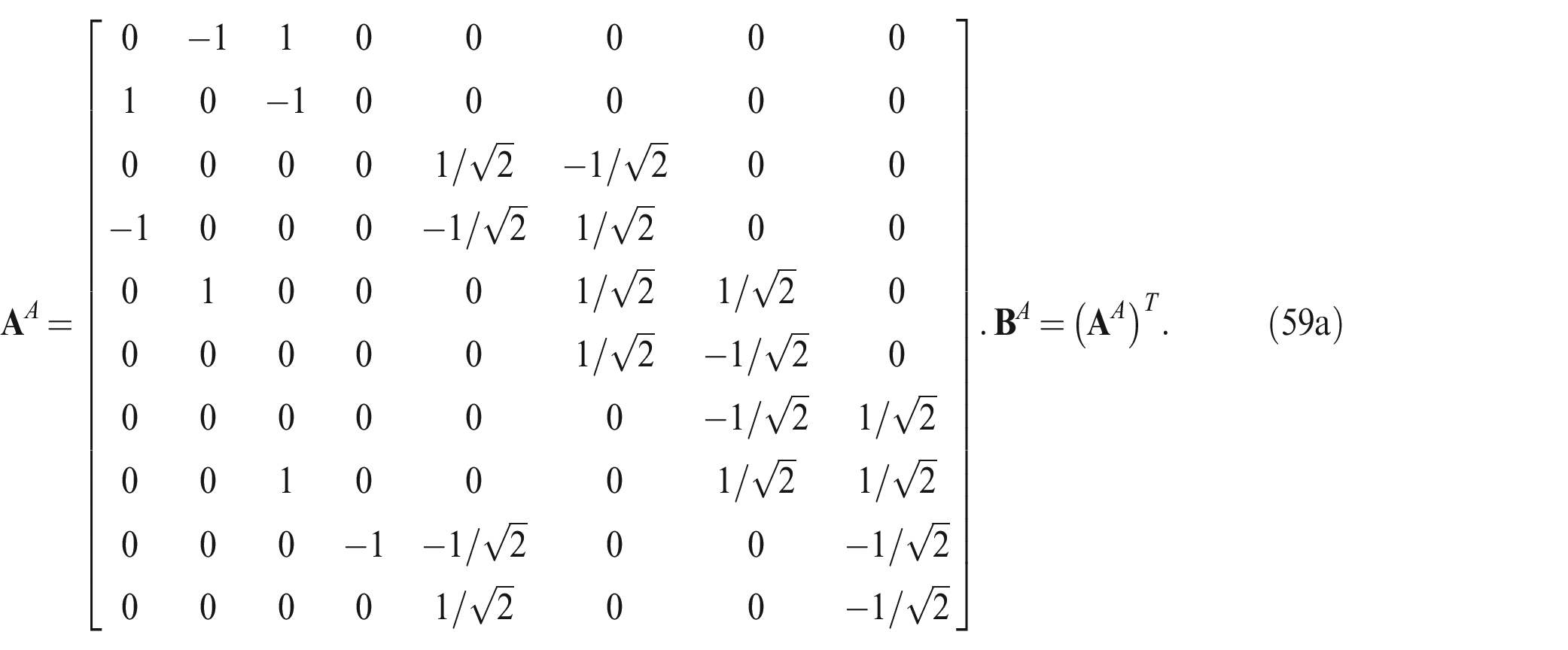
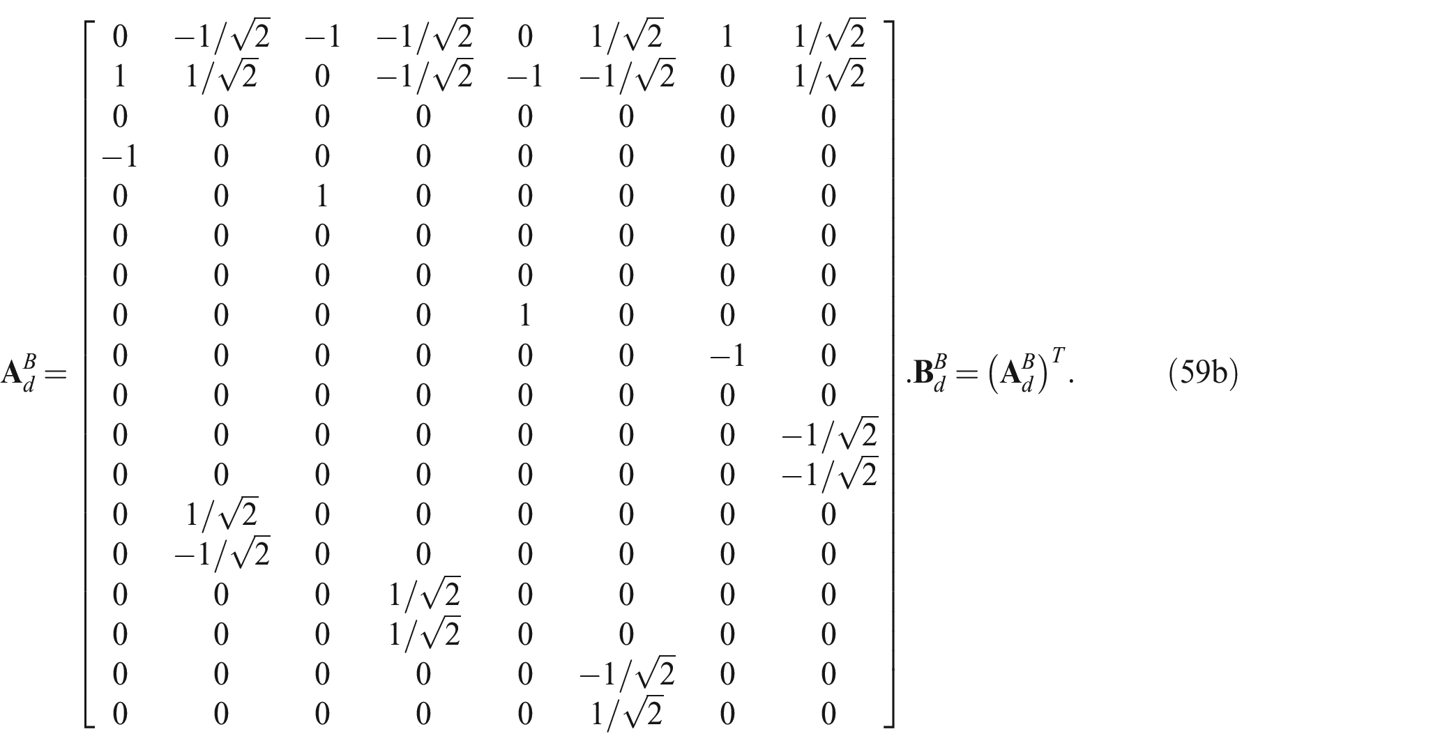
where the equilibrium and kinematic matrices are represented by A and B, respectively. Here, $d$ indicates the DOF related to the dummy nodes. The superscript symbol $T$ indicates the matrix transpose.

The matrix structure $A_{d}^{B}$ , as expressed in Equation (59b), features a dotted rectangle that signifies the modes present with respect to equilibrium matrix row space. These modes are linked to dummy nodes and are subsequently removed to derive the matrix outlined as $A^{B}$ in Equation (60). It is also noted that there is a transpose relation between the equilibrium and kinematic matrices, evident by the virtual work principle [42].

\begin{matrix} A^{B} = [\begin{matrix} 0 & - 1 / \sqrt{2} & - 1 & - 1 / \sqrt{2} & 0 & 1 / \sqrt{2} & 1 & 1 / \sqrt{2} \\ 1 & 1 / \sqrt{2} & 0 & - 1 / \sqrt{2} & - 1 & - 1 / \sqrt{2} & 0 & 1 / \sqrt{2} \\ 0 & 0 & 0 & 0 & 0 & 0 & 0 & 0 \\ - 1 & 0 & 0 & 0 & 0 & 0 & 0 & 0 \\ 0 & 0 & 1 & 0 & 0 & 0 & 0 & 0 \\ 0 & 0 & 0 & 0 & 0 & 0 & 0 & 0 \\ 0 & 0 & 0 & 0 & 0 & 0 & 0 & 0 \\ 0 & 0 & 0 & 0 & 1 & 0 & 0 & 0 \\ 0 & 0 & 0 & 0 & 0 & 0 & - 1 & 0 \\ 0 & 0 & 0 & 0 & 0 & 0 & 0 & 0 \end{matrix}] . \\ B^{B} = {(A^{B})}^{T} . \end{matrix}}

(60)

Upon formulating the equilibrium and kinematic systems, the dependency relationships, as outlined in Table 3, are utilized to facilitate the implementation of Bloch’s wave reduction at respective wave numbers, as presented in Table 4. Subsequently, an analysis of determinacy is conducted on the infinite lattice structure. The results of this analysis on a pin-jointed infinite lattice, as illustrated in Figure 5(a), indicate that the nature of the structure is statically indeterminate but, on the contrary, kinematically determinate. Thus, this classification observed can guide us in concluding that structure is stretching-dominated.

In the subsequent phase, the kinematic boundary based on the Cauchy–Born condition discussed in Equation (25) was utilized to formulate matrix $E$ as:

E^{B} = [\begin{matrix} 0 & 0 & 0 \\ 0 & 0 & 0 \\ 0 & 0 & 0 \\ 0 & 0 & 0 \\ 1 & 0 & 0.5 \\ 0 & 1 & 0.5 \\ 0 & 0 & 1 \\ 0 & 2 & 0 \\ - 1 & 0 & 0.5 \\ 0 & 1 & - 0.5 \\ 0 & 0 & 0 \\ 0 & 0 & 0 \\ 0 & 0 & 0 \\ 0 & 0 & 0 \\ 1 & 0 & 0.5 \\ 0 & 1 & 0.5 \\ - 1 & 0 & 0.5 \\ 0 & 1 & - 0.5 \end{matrix}] . E^{A} = [\begin{matrix} 0 & 0 & 0 \\ 0 & 0 & 0 \\ 0 & 0 & 0 \\ 0 & 0 & 0 \\ 1 & 0 & 0.5 \\ 0 & 1 & 0.5 \\ 0 & 0 & 1 \\ 0 & 2 & 0 \\ - 1 & 0 & 0.5 \\ 0 & 1 & - 0.5 \end{matrix}] .

(61)

The matrix system deduced from the above-derived transformation matrix $E$ is given in Equation (26). The procedure is as follows:

[\begin{matrix} 0 & 1 & 0 & - 1 \\ - 1 & 0 & 1 & 0 \\ 0 & - 1 & 0 & 1 \\ 1 & 0 & - 1 & 0 \\ 0 & 0 & 0 & 0 \\ 0 & 0 & 0 & 0 \\ 0 & 0 & 0 & 0 \\ 0 & 0 & 0 & 0 \end{matrix}] {⌈ \begin{matrix} d_{1 x} \\ d_{1 y} \\ d_{2 x} \\ d_{2 y} \end{matrix} ⌉}^{A} + [\begin{matrix} 0 & 0 & 0 \\ 1 & 0 & 0.5 \\ 0 & 2 & 0 \\ 1 & 0 & - 0.5 \\ 1 / \sqrt{2} & 1 / \sqrt{2} & - 1 / \sqrt{2} \\ 1 / \sqrt{2} & 1 / \sqrt{2} & 1 / \sqrt{2} \\ 1 / \sqrt{2} & 1 / \sqrt{2} & - 1 / \sqrt{2} \\ 1 / \sqrt{2} & 1 / \sqrt{2} & 1 / \sqrt{2} \end{matrix}] ⌈ \begin{matrix} {\bar{ε}}_{xx} \\ {\bar{ε}}_{yy} \\ {\bar{ε}}_{xy} \end{matrix} ⌉ = {⌈ \begin{matrix} e_{1} \\ e_{2} \\ e_{3} \\ e_{4} \\ e_{5} \\ e_{6} \\ e_{7} \\ e_{8} \end{matrix} ⌉}^{A} .

(62a)

[\begin{matrix} 0 & 1 & 0 & - 1 \\ - 1 / \sqrt{2} & 1 / \sqrt{2} & 0 & 0 \\ - 1 & 0 & 1 & 0 \\ - 1 / \sqrt{2} & - 1 / \sqrt{2} & 0 & 0 \\ 0 & - 1 & 0 & 1 \\ 1 / \sqrt{2} & - 1 / \sqrt{2} & 0 & 0 \\ 1 & 0 & - 1 & 0 \\ 1 / \sqrt{2} & 1 / \sqrt{2} & 0 & 0 \end{matrix}] {⌈ \begin{matrix} d_{1 x} \\ d_{1 y} \\ d_{2 x} \\ d_{2 y} \end{matrix} ⌉}^{B} + [\begin{matrix} 0 & 0 & 0 \\ 0 & 0 & 0 \\ 1 & 0 & 0.5 \\ 1 / \sqrt{2} & 1 / \sqrt{2} & 1 / \sqrt{2} \\ 0 & 2 & 0 \\ 1 / \sqrt{2} & 1 / \sqrt{2} & - 1 / \sqrt{2} \\ 1 & 0 & - 0.5 \\ 0 & 0 & 0 \end{matrix}] ⌈ \begin{matrix} {\bar{ε}}_{xx} \\ {\bar{ε}}_{yy} \\ {\bar{ε}}_{xy} \end{matrix} ⌉ = {⌈ \begin{matrix} e_{1} \\ e_{2} \\ e_{3} \\ e_{4} \\ e_{5} \\ e_{6} \\ e_{7} \\ e_{8} \end{matrix} ⌉}^{B} .

(62b)

The above matrices aid in the description of the element deformations as a function of the macroscopic strain field as:

{⌈ \begin{matrix} e_{1} \\ e_{2} \\ e_{3} \\ e_{4} \\ e_{5} \\ e_{6} \\ e_{7} \\ e_{8} \end{matrix} ⌉}^{B} = [\begin{matrix} 0 & 1 & 0 \\ 1 / (2 \sqrt{2}) & 1 / (2 \sqrt{2}) & - 1 / (2 \sqrt{2}) \\ 1 & 0 & 0 \\ 1 / (2 \sqrt{2}) & 1 / (2 \sqrt{2}) & 1 / (2 \sqrt{2}) \\ 0 & 1 & 0 \\ 1 / (2 \sqrt{2}) & 1 / (2 \sqrt{2}) & - 1 / (2 \sqrt{2}) \\ 1 & 0 & 0 \\ 1 / (2 \sqrt{2}) & 1 / (2 \sqrt{2}) & 1 / (2 \sqrt{2}) \end{matrix}] ⌈ \begin{matrix} {\bar{ε}}_{xx} \\ {\bar{ε}}_{yy} \\ {\bar{ε}}_{xy} \end{matrix} ⌉ .

{⌈ \begin{matrix} e_{1} \\ e_{2} \\ e_{3} \\ e_{4} \\ e_{5} \\ e_{6} \\ e_{7} \\ e_{8} \end{matrix} ⌉}^{A} = [\begin{matrix} 0 & 1 & 0 \\ 1 & 0 & 0 \\ 0 & 1 & 0 \\ 1 & 0 & 0 \\ 1 / \sqrt{2} & 1 / \sqrt{2} & - 1 / \sqrt{2} \\ 1 / \sqrt{2} & 1 / \sqrt{2} & 1 / \sqrt{2} \\ 1 / \sqrt{2} & 1 / \sqrt{2} & - 1 / \sqrt{2} \\ 1 / \sqrt{2} & 1 / \sqrt{2} & 1 / \sqrt{2} \end{matrix}] ⌈ \begin{matrix} {\bar{ε}}_{xx} \\ {\bar{ε}}_{yy} \\ {\bar{ε}}_{xy} \end{matrix} ⌉ .

(63)

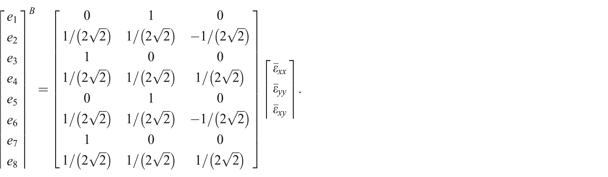
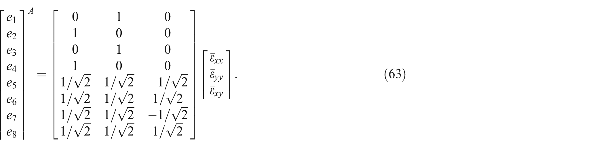
The strain energy densities of unit cells A and B are obtained by utilizing the deformation vectors of respective cell elements. These deformation vectors are indicated in Equation (63). The next step involves the application of Castigliano’s theorem to the lattice, forming the homogenized stiffness matrix. For the lattice material, it can be determined that the fourth order, homogenized stiffness tensor obtained from both the deformation vectors are similar.

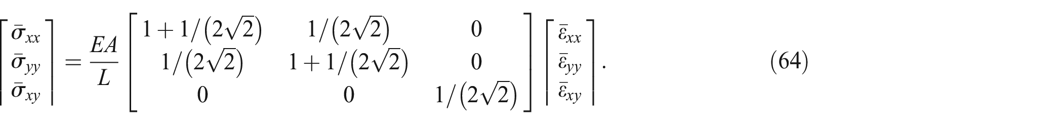
⌈ \begin{matrix} {\bar{σ}}_{xx} \\ {\bar{σ}}_{yy} \\ {\bar{σ}}_{xy} \end{matrix} ⌉ = \frac{EA}{L} [\begin{matrix} 1 + 1 / (2 \sqrt{2}) & 1 / (2 \sqrt{2}) & 0 \\ 1 / (2 \sqrt{2}) & 1 + 1 / (2 \sqrt{2}) & 0 \\ 0 & 0 & 1 / (2 \sqrt{2}) \end{matrix}] ⌈ \begin{matrix} {\bar{ε}}_{xx} \\ {\bar{ε}}_{yy} \\ {\bar{ε}}_{xy} \end{matrix} ⌉ .

(64)

The outcome presented herein showcases the precision of the DNR and the elimination methodology.

5.2. Example 2—Lattice structure with Schlafli symbol of 3³.4²

The lattice structure indicated in Figure 7 is analyzed in this section.

Figure 7.

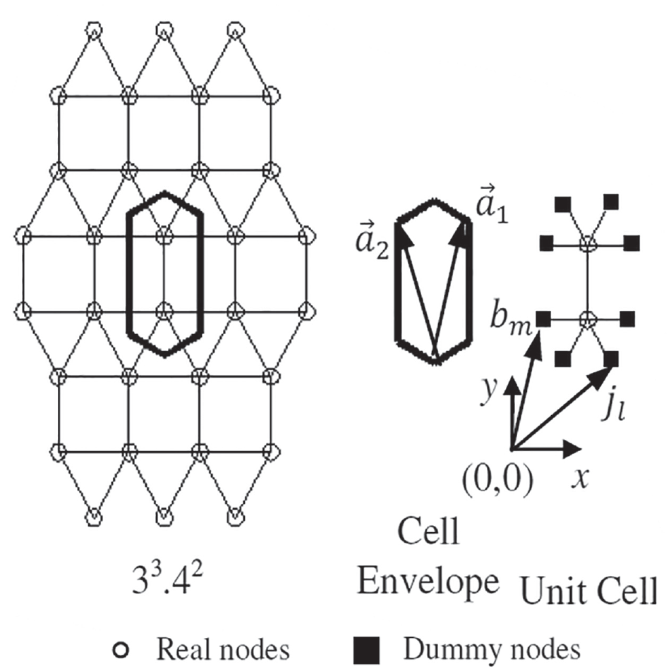
2D semi-regular 3³.4² lattice structure.

5.2.1. Equilibrium System at the Unit Cell level

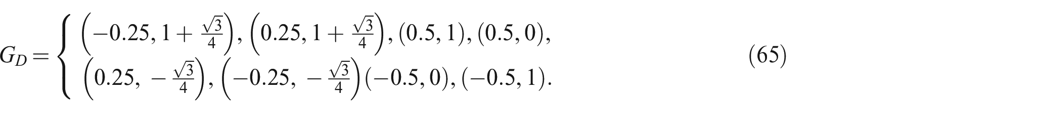
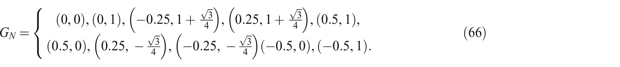
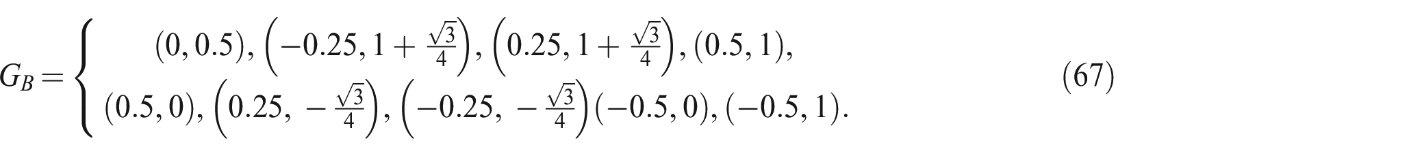
The bases groups involved in the unit cell finite structure include

Dummy node bases group $(G_{D}$ ):

G_{D} = {\begin{matrix} (- 0.25, 1 + \frac{\sqrt{3}}{4}), (0.25, 1 + \frac{\sqrt{3}}{4}), (0.5, 1), (0.5, 0), \\ (0.25, - \frac{\sqrt{3}}{4}), (- 0.25, - \frac{\sqrt{3}}{4}) (- 0.5, 0), (- 0.5, 1) . \end{matrix}

(65)

Node bases group ( $G_{N}$ ):

G_{N} = {\begin{matrix} (0, 0), (0, 1), (- 0.25, 1 + \frac{\sqrt{3}}{4}), (0.25, 1 + \frac{\sqrt{3}}{4}), (0.5, 1), \\ (0.5, 0), (0.25, - \frac{\sqrt{3}}{4}), (- 0.25, - \frac{\sqrt{3}}{4}) (- 0.5, 0), (- 0.5, 1) . \end{matrix}

(66)

Bar bases group (G_B):

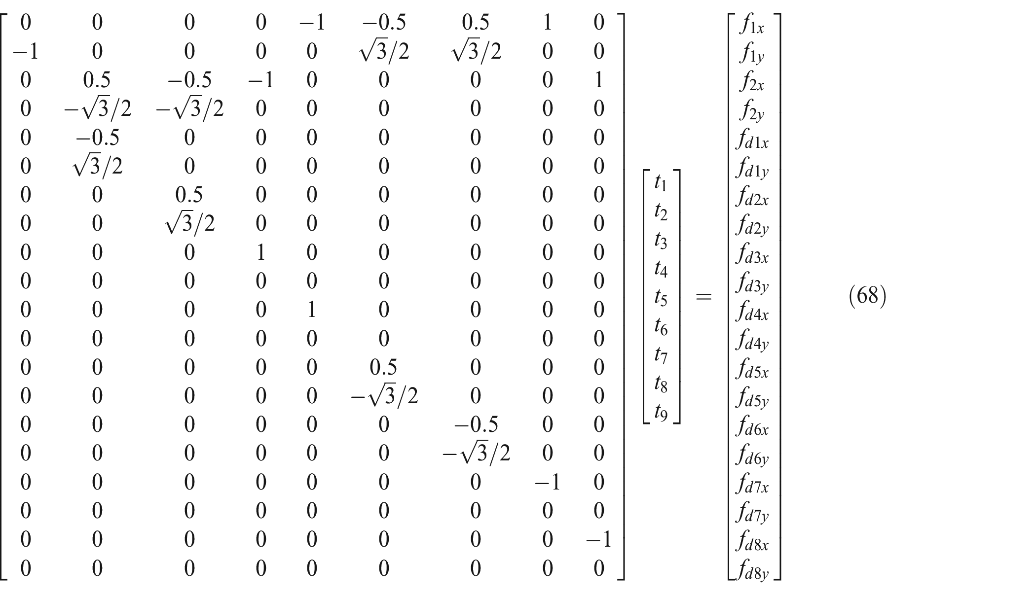
G_{B} = {\begin{matrix} (0, 0.5), (- 0.25, 1 + \frac{\sqrt{3}}{4}), (0.25, 1 + \frac{\sqrt{3}}{4}), (0.5, 1), \\ (0.5, 0), (0.25, - \frac{\sqrt{3}}{4}), (- 0.25, - \frac{\sqrt{3}}{4}) (- 0.5, 0), (- 0.5, 1) . \end{matrix}

(67)

The equilibrium system of the unit cell is obtained below after the application of the DNR approach, where the DOFs of the dummy are also included.

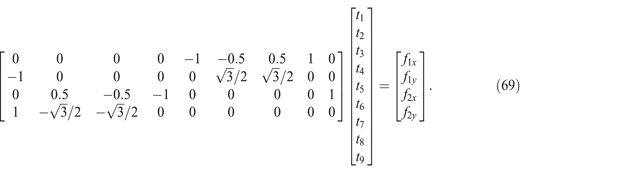
[\begin{matrix} 0 & 0 & 0 & 0 & - 1 & - 0.5 & 0.5 & 1 & 0 \\ - 1 & 0 & 0 & 0 & 0 & \sqrt{3} / 2 & \sqrt{3} / 2 & 0 & 0 \\ 0 & 0.5 & - 0.5 & - 1 & 0 & 0 & 0 & 0 & 1 \\ 0 & - \sqrt{3} / 2 & - \sqrt{3} / 2 & 0 & 0 & 0 & 0 & 0 & 0 \\ 0 & - 0.5 & 0 & 0 & 0 & 0 & 0 & 0 & 0 \\ 0 & \sqrt{3} / 2 & 0 & 0 & 0 & 0 & 0 & 0 & 0 \\ 0 & 0 & 0.5 & 0 & 0 & 0 & 0 & 0 & 0 \\ 0 & 0 & \sqrt{3} / 2 & 0 & 0 & 0 & 0 & 0 & 0 \\ 0 & 0 & 0 & 1 & 0 & 0 & 0 & 0 & 0 \\ 0 & 0 & 0 & 0 & 0 & 0 & 0 & 0 & 0 \\ 0 & 0 & 0 & 0 & 1 & 0 & 0 & 0 & 0 \\ 0 & 0 & 0 & 0 & 0 & 0 & 0 & 0 & 0 \\ 0 & 0 & 0 & 0 & 0 & 0.5 & 0 & 0 & 0 \\ 0 & 0 & 0 & 0 & 0 & - \sqrt{3} / 2 & 0 & 0 & 0 \\ 0 & 0 & 0 & 0 & 0 & 0 & - 0.5 & 0 & 0 \\ 0 & 0 & 0 & 0 & 0 & 0 & - \sqrt{3} / 2 & 0 & 0 \\ 0 & 0 & 0 & 0 & 0 & 0 & 0 & - 1 & 0 \\ 0 & 0 & 0 & 0 & 0 & 0 & 0 & 0 & 0 \\ 0 & 0 & 0 & 0 & 0 & 0 & 0 & 0 & - 1 \\ 0 & 0 & 0 & 0 & 0 & 0 & 0 & 0 & 0 \end{matrix}] [\begin{matrix} t_{1} \\ t_{2} \\ t_{3} \\ t_{4} \\ t_{5} \\ t_{6} \\ t_{7} \\ t_{8} \\ t_{9} \end{matrix}] = [\begin{matrix} f_{1 x} \\ f_{1 y} \\ f_{2 x} \\ f_{2 y} \\ f_{d 1 x} \\ f_{d 1 y} \\ f_{d 2 x} \\ f_{d 2 y} \\ f_{d 3 x} \\ f_{d 3 y} \\ f_{d 4 x} \\ f_{d 4 y} \\ f_{d 5 x} \\ f_{d 5 y} \\ f_{d 6 x} \\ f_{d 6 y} \\ f_{d 7 x} \\ f_{d 7 y} \\ f_{d 8 x} \\ f_{d 8 y} \end{matrix}]

(68)

After the elimination of the DOFs of the dummy nodes, the matrix reduces to:

[\begin{matrix} 0 & 0 & 0 & 0 & - 1 & - 0.5 & 0.5 & 1 & 0 \\ - 1 & 0 & 0 & 0 & 0 & \sqrt{3} / 2 & \sqrt{3} / 2 & 0 & 0 \\ 0 & 0.5 & - 0.5 & - 1 & 0 & 0 & 0 & 0 & 1 \\ 1 & - \sqrt{3} / 2 & - \sqrt{3} / 2 & 0 & 0 & 0 & 0 & 0 & 0 \end{matrix}] [\begin{matrix} t_{1} \\ t_{2} \\ t_{3} \\ t_{4} \\ t_{5} \\ t_{6} \\ t_{7} \\ t_{8} \\ t_{9} \end{matrix}] = [\begin{matrix} f_{1 x} \\ f_{1 y} \\ f_{2 x} \\ f_{2 y} \end{matrix}] .

(69)

5.2.2. Determinacy Analysis of Unit Cell Finite Structure

After computing the four fundamental subspaces of the equilibrium matrix of the unit cell, it can be inferred that the unit cell is statically determinate and kinematically indeterminate with 11 modes of mechanisms, of which three are rigid-body mechanisms and eight are internal mechanisms.

5.2.3. Infinite Lattice Determinacy Analysis

Direct translational bases:

${\vec{a}}_{1} = (0.5, 1 + \frac{\sqrt{3}}{2})$ .

${\vec{a}}_{2} = (- 0.5, 1 + \frac{\sqrt{3}}{2})$ .

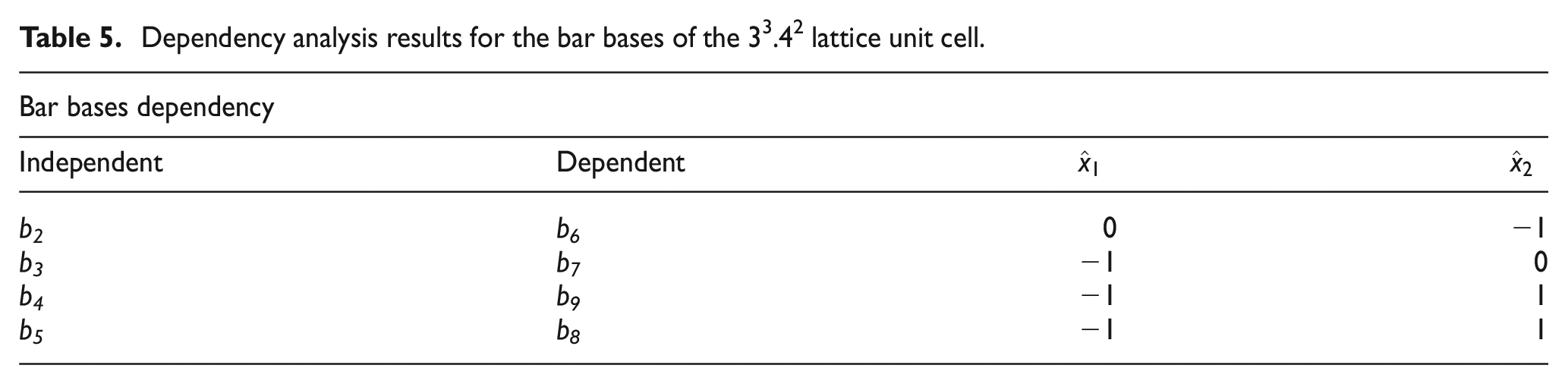
It is deduced that all real nodes are independent of the dependency analysis of the bar and node bases groups. The bar dependency relations are indicated in Table 5.

Table 5.

Dependency analysis results for the bar bases of the 3³.4² lattice unit cell.

Bar bases dependency
Independent	Dependent	${\hat{x}}_{1}$	${\hat{x}}_{2}$
b ₂	b ₆	0	−1
b ₃	b ₇	−1	0
b ₄	b ₉	−1	1
b ₅	b ₈	−1	1

The reciprocal lattice bases:

${\vec{b}}_{1}$ = (1, 0.2679).

${\vec{b}}_{2}$ = (− 1, 0.2679).

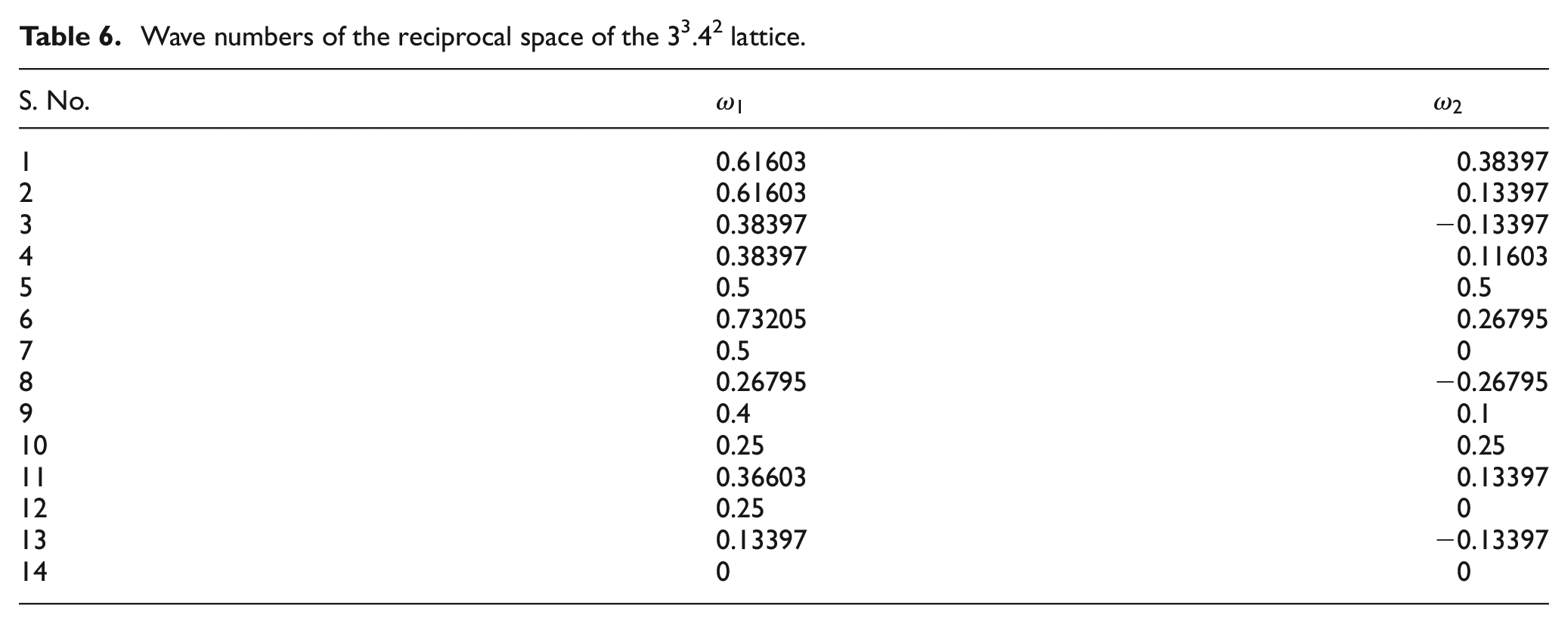
The reciprocal lattice bases are used to construct the reciprocal lattice and the first Brillouin zone, whereas the point group symmetry is used to determine the first IBZ as shown in Figure 8. The associated wave numbers are listed in Table 6.

Figure 8.

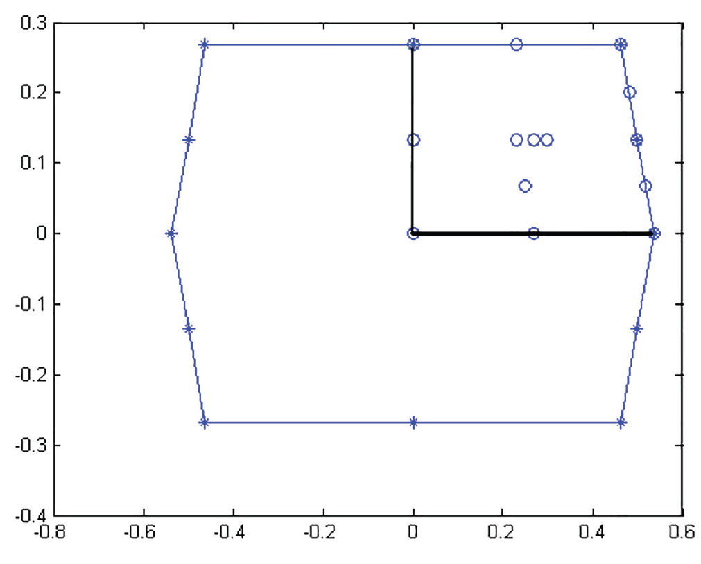
The first Brillouin zone and the first irreducible Brillouin zone of the 3³.4² lattice.

Table 6.

Wave numbers of the reciprocal space of the 3³.4² lattice.

S. No.	$ω_{1}$	$ω_{2}$
1	0.61603	0.38397
2	0.61603	0.13397
3	0.38397	−0.13397
4	0.38397	0.11603
5	0.5	0.5
6	0.73205	0.26795
7	0.5	0
8	0.26795	−0.26795
9	0.4	0.1
10	0.25	0.25
11	0.36603	0.13397
12	0.25	0
13	0.13397	−0.13397
14	0	0

From the dependency relations listed in Table 5, transformation matrices are formed which are required to reduce the equilibrium system of the unit cell to the irreducible form of the infinite lattice at each wave number, as given in Table 6. These are then used for the determinacy analysis of the infinite lattice structure. The results of the determinacy analysis of the infinite 3³.4² lattice are listed in Table 7.

Table 7.

Determinacy analysis results for the 3³.4² lattice.

Wave numbers		SSS	SIM
$ω_{1}$	$ω_{2}$	SSS	SIM
0.61603	0.38397	1	0
0.61603	0.13397	1	0
0.38397	−0.13397	1	0
0.38397	0.11603	1	0
0.5	0.5	2	1
0.73205	0.26795	1	0
0.5	0	1	0
0.26795	−0.26795	1	0
0.4	0.1	1	0
0.25	0.25	2	1
0.36603	0.13397	1	0
0.25	0	1	0
0.13397	−0.13397	1	0
0	0	3	2

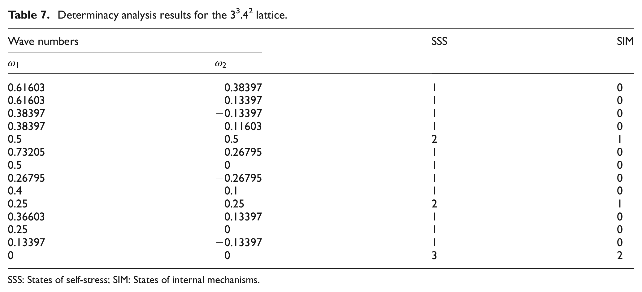
SSS: States of self-stress; SIM: States of internal mechanisms.

The results indicate that the 3³.4² infinite lattice is statically and kinematically indeterminate at wave numbers $ω$ = (0.25,0.25), $ω$ = (0.5,0.5), and $ω$ = (0,0); and statically indeterminate and kinematically determinate at all other wave numbers.

6. Conclusion

The paper presents the DNR as a method for evaluating the effective properties of pin-jointed lattice structures that feature the envelope of the unit cells coinciding with the constituent cell elements at points not essentially at the end nodes, thereby expanding the efficiency and modeling capability for geometries of complex nature. In the case of certain lattices, the article, in addition, introduced an approach for implementing the principle in assessing determinacy and the homogenization of the stiffness properties. Two examples of lattice structures have been described in detail, with the agreement of the obtained results to those existing in the literature, validating the methodology described in this paper. Any pin-jointed lattice topology may be analyzed and characterized in an automated manner utilizing the DNR. The DNR approach can also be utilized to evaluate the dynamic characteristics of any discretized mechanical system. The approach is important where periodicity can be applied to the field variables of the kinematic matrix, mass matrix, and equation of motion in the discretized mechanical system. Although this paper considered only 2D pin-jointed lattice structures, future studies can include cases involving 3D pin-jointed lattice geometries, which can also be analyzed straightforwardly by an extension of the developed approach.

Footnotes

Declaration of conflicting interests

The author(s) declared no potential conflicts of interest with respect to the research, authorship, and/or publication of this article.

Funding

The author(s) received no financial support for the research, authorship, and/or publication of this article.

ORCID iDs

Sandeep Suresh Babu

Abdel-Hamid Ismail Mourad

References

Elsayed

MSA

Pasini

. Characterization and performance optimization of 2D lattice materials with hexagonal Bravais lattice symmetry. In: International design engineering technical conferences and computers and information in engineering conference, San Diego, CA, 30 August–2 September 2009, pp. 1315–1323. New York: ASME.

Elsayed

MSA

Pasini

Analysis of the elastostatic specific stiffness of 2D stretching-dominated lattice materials. Mech Mater 2010; 42(7): 709–725.

Wagner

Lumpe

Chen

, et al. Programmable, active lattice structures: unifying stretch-dominated and bending-dominated topologies. Extrem Mech Lett 2019; 29: 100461.

Deshpande

Ashby

Fleck

NA.

Foam topology: bending versus stretching dominated architectures. Acta Mater 2001; 49(6): 1035–1040.

Alkhader

Nazzal

Louca

Design of bending dominated lattice architectures with improved stiffness using hierarchy. Proc Inst Mech Eng Part C J Mech Eng Sci 2019; 233(11): 3976–3993.

Zhong

Song

, et al. The Gibson-Ashby model for additively manufactured metal lattice materials: its theoretical basis, limitations and new insights from remedies. Curr Opin Solid State Mater Sci 2023; 27(3): 101081.

Maxwell

JC.

L. on the calculation of the equilibrium and stiffness of frames. London Edinburgh. Dublin Philos Mag J Sci 1864; 27(182): 294–299.

Chen

Watts

Jackson

, et al. Stiff isotropic lattices beyond the Maxwell criterion. Sci Adv 2019; 5(9): eaaw1937.

Calladine

CR.

Buckminster Fuller’s “tensegrity” structures and Clerk Maxwell’s rules for the construction of stiff frames. Int J Solids Struct 1978; 14(2): 161–172.

10.

Pellegrino

Calladine

CR.

Matrix analysis of statically and kinematically indeterminate frameworks. Int J Solids Struct 1986; 22(4): 409–428.

11.

Arabnejad

Pasini

Mechanical properties of lattice materials via asymptotic homogenization and comparison with alternative homogenization methods. Int J Mech Sci 2013; 77: 249–262.

12.

Dos Reis

Karathanasopoulos

Inverse metamaterial design combining genetic algorithms with asymptotic homogenization schemes. Int J Solids Struct 2022; 250: 111702.

13.

Barchiesi

Eugster

dell’Isola

, et al. Large in-plane elastic deformations of bi-pantographic fabrics: asymptotic homogenization and experimental validation. Math Mech Solids 2020; 25(3): 739–767.

14.

Barchiesi

Spagnuolo

Placidi

Mechanical metamaterials: a state of the art. Math Mech Solids 2018; 24(1): 212–234.

15.

Boutin

Hans

Homogenisation of periodic discrete medium: application to dynamics of framed structures. Comput Geotech 2003; 30(4): 303–320.

16.

Hans

Boutin

Dynamics of discrete framed structures: a unified homogenized description. J Mech Mater Struct 2008; 3(9): 1709–1739.

17.

D’Annibale

Ferretti

Luongo

Static and dynamic responses of micro-structured beams. Appl Sci 2020; 10(19): 6836.

18.

Ferretti

D’Annibale

Buckling of planar micro-structured beams. Appl Sci 2020; 10(18): 6506.

19.

Sepehri

Mashhadi

Fakhrabadi

MMS

. Size-dependent wave propagation in two-dimensional functionally graded lattice materials. Int J Mech Sci 2022; 232: 107605.

20.

Gasparetto

VEL

ElSayed

MSA

. Multiscale optimization of specific elastic properties and microscopic frequency band-gaps of architectured microtruss lattice materials. Int J Mech Sci 2021; 197: 106320.

21.

Herzog-Arbeitman

Chew

Bernevig

BA.

Magnetic Bloch theorem and reentrant flat bands in twisted bilayer graphene at 2 π flux. Phys Rev B 2022; 106(8): 085140.

22.

Sepehri

Mashhadi

Fakhrabadi

MMS

. Out-of-plane wave propagation in two-dimensional micro-lattices. Phys Scr 2021; 96(8): 085704.

23.

Pan

Han

Design and optimization of lattice structures: a review. Appl Sci 2020; 10(18): 6374.

24.

Born

Wave propagation in periodic structures. Nature 1946; 158(4026): 926.

25.

Wang

Cai

Zhou

, et al. Homogenization in a simpler way: analysis and optimization of periodic unit cells with Cauchy–Born hypothesis. Struct Multidiscip Optim 2021; 64: 3911–3935.

26.

Andrea

Margherita

, et al. Beyond the classical Cauchy-Born rule. arXiv preprint, 2022, https://arxiv.org/abs/2210.06147

27.

Dai

Wang

Yang

, et al. On the Cauchy-Born approximation at finite temperature for alloys. Discret Contin Dyn Syst 2022; 27(6): 3131–3153.

28.

Somnic

BW.

Status and challenges in homogenization methods for lattice materials. Materials 2022; 15(2): 605.

29.

Somnic

BW.

Homogenization methods of lattice materials. Encyclopedia 2022; 2(2): 1091–1102.

30.

Chen

Yan

Sareh

, et al. Nodal flexibility and kinematic indeterminacy analyses of symmetric tensegrity structures using orbits of nodes. Int J Mech Sci 2019; 155: 41–49.

31.

Xia

Xiao

Chen

, et al. Determination of static and kinematic determinacy of pin-jointed assemblies using rigid-body displacements as primary unknown variables. Eng Struct 2019; 181: 643–652.

32.

Elsayed

MSA.

Multiscale mechanics and structural design of periodic cellular materials. Montreal, QC, Canada: McGill University, 2010.

33.

Bhattacharya

Microstructure of martensite: why it forms and how it gives rise to the shape-memory effect. Vol. 2. Oxford: Oxford University Press, 2003.

34.

Maconachie

Leary

Lozanovski

, et al. SLM lattice structures: properties, performance, applications and challenges. Mater Des 2019; 183: 108137.

35.

Dang

Duan

, et al. Deployment kinematics of axisymmetric Miura origami: unit cells, tessellations, and stacked metamaterials. Int J Mech Sci 2022; 232: 107615.

36.

Zhang

Guo

, et al. Numerical investigation of impact behavior of strut-based cellular structures designed by spatial Voronoi tessellation. Metals 2022; 12(7): 1189.

37.

Hutchinson

Fleck

NA.

The structural performance of the periodic truss. J Mech Phys Solids 2006; 54(4): 756–782.

38.

Bhat

Kumar

Lin

, et al. A novel bioinspired architectured materials with interlocking designs based on tessellation. Addit Manuf 2022; 58: 103052.

39.

Jorgensen

Christensen

Jarvis

, et al. A general algorithm for calculating irreducible Brillouin zones. arXiv Preprint, 2021, https://arxiv.org/abs/2104.05856

40.

Vasseur

JO.

Periodic structures, irreducible Brillouin zone, dispersion relations and the plane wave expansion method. In: Jiménez

Umnova

Groby

J-P

(eds) Acoust Waves Period Struct Metamaterials, Porous Media. New York: Springer, 2021, pp. 3–42.

41.

Yang

Yun

Cao

YJ.

Irreducible first Brillouin zone for two-dimensional magnonic crystals with asymmetric complex lattices. Mod Phys Lett B 2021; 35(10): 2150170.

42.

Elsayed

MSA

Pasini

. The Bloch’s Theorem, Technical Report No. TR-MDOG-09-01, 2009. Montreal, QC, Canada: McGill University.

43.

De Gennaro

Colonna

Linscott

, et al. Bloch’s theorem in orbital-density-dependent functionals: band structures from Koopmans spectral functionals. Phys Rev B 2022; 106(3): 035106.

44.

Hosseini

Zhang

Band structure analysis of Green-Naghdi-based thermoelastic wave propagation in cylindrical phononic crystals with energy dissipation using a meshless collocation method. Int J Mech Sci 2021; 209: 106711.

45.

Zhang

Bloch’s band structures of a pair of interacting electrons in simple one-and two-dimensional lattices. Phys Lett A 2021; 414: 127634.

46.

Kuznetsov

EN.

On the evaluation of statical-kinematic stiffness matrix for underconstrained structural systems. Int J Solids Struct 2000; 37(15): 2215–2223.

47.

Kuznetsov

EN.

Orthogonal load resolution and statical-kinematic stiffness matrix. Int J Solids Struct 1997; 34(28): 3657–3672.

Extended Dummy Node Rule for analysis and characterization of pin-jointed periodic cellular materials: An approach based on Bloch-wave method

Abstract

Keywords

1. Introduction

2. Mathematical description of a lattice structure

2.1. Lattice bases

2.1.1. Dummy Node Bases Group

2.1.2. Node Bases Group

A.3 Bar Bases Group

2.2. Direct translational bases

2.3. Direct translational vector

2.4. Position vectors

2.5. Direct lattice

2.6. Reciprocal lattice

2.7. Bloch’s theorem

2.7.1. Bloch wave function

3. The DNR

3.1. Proof of the DNR

4. Dummy node elimination scheme—DNR application

4.1. Determinacy analysis of lattice structure

4.1.1. Equilibrium and Kinematic Matrices—Formulation with respect to a unit cell

4.2. Derivation of the Cauchy–Born kinematic boundary condition: Homogenization of the mechanical properties of the lattice microstructure

4.3. Elimination scheme—proof and validation

4.3.1. Equilibrium Analysis

4.3.2. Kinematic Analysis

5. Applications

5.1. Example 1

5.2. Example 2—Lattice structure with Schlafli symbol of 33.42

5.2.1. Equilibrium System at the Unit Cell level

5.2.2. Determinacy Analysis of Unit Cell Finite Structure

5.2.3. Infinite Lattice Determinacy Analysis

6. Conclusion

Footnotes

Declaration of conflicting interests

Funding

ORCID iDs

References

5.2. Example 2—Lattice structure with Schlafli symbol of 3³.4²