Metal plasticity and nonlocal damage modeling: A thermodynamically consistent GSM approach with computational implications

Abstract

This paper presents a comprehensive analysis of generalized standard materials (GSMs), with a particular focus on their application to metal plasticity and nonlocal damage models. Building on the foundational work of Halphen and Nguyen, the GSM framework is explored in the contexts of both small strain von Mises plasticity and advanced models for ductile fracture, such as the GLD framework, which incorporates cavity shape effects and nonlocal interactions. The study addresses key challenges, including the numerical stability and convergence of finite element implementations, with simulations of compact tension (CT) specimen fracture tests for two different steels demonstrating the accuracy and predictive capability of the GLD model. In addition, the paper delves into nonlocal damage models, presenting two key theoretical results: the attenuation of high-frequency components, where Gaussian kernels act as low-pass filters, and the connection of nonlocal formulations to a diffusion-like equation. A modified evolution equation with logarithmic terms is proposed to address excessive smoothing, and a sensitivity analysis of the length scale parameter l provides practical guidelines for optimizing nonlocal formulations for realistic damage simulation while maintaining numerical stability.

Keywords

Generalized standard materials thermodynamic consistency plasticity projection problem metal plasticity nonlocal damage models

1. Introduction

The formalism of generalized standard materials (GSMs) was first introduced by Halphen and Nguyen [1] in the context of elasto-plasticity. In short, the constitutive equations of GSM are described by the expressions of the elastic energy density (also called reversible elastic potential) and the dissipation potential. The elastic energy density, stored in the material by its deformation under external stimuli, provides by derivation of the Cauchy stress and the thermodynamics forces, while the dissipation potential, gives rise to the evolution equations of the internal state variables. The formalism GSM was developed within the framework of linearized theory and is suitable for rate-independent materials. Although these two restrictions may limit the use of this formalism to describe a vast majority of materials and their behaviors under various external conditions, the success credited to the GSM approach is tremendous in view of the nice local and global stability properties it offers for robust numerical implementations in finite-element subroutines. Of course, for other materials, additional precautions are required to guarantee local and global stabilities of numerical schemes, since the tangent stiffness matrix can become non-invertible during nonlinear analyses.

Initially developed in the context of small strain rate independent elasto-plasticity by Halphen and Nguyen [1] and later on reviewed by Ziegler and Wehrli [2], the GSM formalism was extended to finite strain elasto-plasticity by Hackl [3]. The later extension was proposed as an alternative theoretical framework to overcome the usual problems encountered in the use of classical finite elasto-plasticity models. These problems include arbitrariness in the choice of yield functions and flow rules, difficulty to obtain a clear distinction between the concept of frame indifference and material symmetry which is complicated by the unclear role played by the introduction of the intermediate configuration¹, and generally non-equivalence between the yield functions obtained in the different configurations introduced by the adoption of a multiplicative decomposition of the deformation gradient, refer Lee [4]. Once developed, the GSM framework has continuously played a key role in the modeling of materials, refer Hackl [3], Fremond [5], Maugin [6] among other authors, and ductile fracture in porous solids, refer Enakoutsa et al. [7]. The application of this formalism to metal plasticity, whether governed by the classical von Mises model or advanced models such as the nonolocal GLD framework for ductile fracture, which incorporates cavity shape effects under the linearized theory assumption, or within the context of J₂ plasticity, has been sparsely explored in the literature. The limited attention given to these formulations highlights the need for further investigation into their thermodynamics consistency and numerical implementation. This study aims to rigorously bridge this gap by developing a comprehensive analysis of these models and their implications. In particular, we will analyze the relationship between the GSMs framework and metal plasticity models, focusing on the von Mises yield criterion as a foundational case, and extending the analysis to the more complex GLD model for ductile fracture, incorporating cavity shape effects and nonlocal effects.

Moreover, nonlocal damage models have emerged as robust tools in computational mechanics to address challenges associated with mesh sensitivity in simulations involving material softening and strain localization. These models, characterized by their integral-based formulations, effectively regularize the solution by incorporating spatial interactions over a finite domain governed by a kernel function. While this regularization mitigates numerical pathologies such as spurious mesh dependency, it introduces a new challenge: excessive smoothing of the damage variable. This smoothing, often mathematically analogous to diffusion, can lead to physical inconsistencies, such as delayed crack initiation or overly homogenized damage patterns near critical regions like crack tips.

The theoretical basis for this behavior stems from the attenuation of high-frequency components and the implicit connection to diffusion-like processes. Theoretical results presented in this work establish that the Gaussian kernel used in nonlocal models acts as a low-pass filter, suppressing high-wavenumber contributions exponentially. Furthermore, a connection between nonlocal formulations and diffusion equations is derived, offering insights into the regularization mechanism and its implications for numerical stability and accuracy. This understanding lays the groundwork for developing enhanced nonlocal models that balance regularization with physical fidelity.

To address the limitations of excessive smoothing, modifications to the evolution equation are explored. Specifically, a logarithmic reformulation of the damage variable introduces stability while preserving spatial consistency in damage evolution. A rigorous stability analysis confirms that the modified formulation retains its ability to attenuate high-frequency perturbations while avoiding over-smoothing.

Finally, this paper examines the sensitivity of nonlocal models to the length scale parameter l, which governs the spatial extent of nonlocal interactions. Analytical tools, including the second moment of the kernel, provide a quantitative measure of the kernel’s influence radius and its impact on the diffusive behavior of the model. By exploring the trade-offs introduced by varying l, this work offers practical guidelines for optimizing nonlocal models to achieve realistic damage simulations.

The outline of the paper is as follows.

Section 2 gives an overview of some of the work of Halphen and Nguyen [1] and Nguyen [8] on GSMs.

Section 3 demonstrates how the constitutive relations of the classical small strain the von Mises model with isotropic hardening defines a generalized standard material. In addition, we discuss the benefits of this property on the numerical implementation of von Mises model into a numerical subroutine using the well-known projection algorithm.

Section 4 offers a thorough analysis of the interaction between the GSMs framework and the constitutive equations of the GLD model for ductile fracture, with a particular emphasis on the mathematical formulation of cavity shape effects. In addition, we address the projection problem that arises in the numerical implementation of the model within a finite-element framework. We establish that, under the assumptions of fixed porosity and a constant cavity shape factor, the projection problem results in a unique solution, thereby ensuring numerical stability and convergence. Furthermore, as a practical application of the GLD model, we present simulations of the fracture behavior of a Compact Test specimen subjected to tensile loading. These simulations align closely with experimental data for the 16 MND and SS 315L stainless steels.

Nonlocal damage models are effective in addressing mesh sensitivity in computational mechanics but often suffer from excessive smoothing, similar to a diffusion process, which may result in unrealistic damage distributions. In Section 4, a theoretical analysis demonstrates that Gaussian kernels in these models exponentially attenuate high-frequency components and closely approximate a diffusion-like equation. To address this issue, a modified evolution equation incorporating logarithmic terms is proposed, enhancing stability and maintaining spatial consistency. In addition, sensitivity analysis of the length-scale parameter l offers practical guidelines for optimizing the balance between regularization and physical accuracy in nonlocal formulations.

2. Overview of the formalism of GSM

In this section, we give a brief summary of some aspects of the works of Halphen and Nguyen [1] and Nguyen [8] on GSM. The theory is applicable only in the context of linearized theory.

The constitutive law of a generalized standard material is described by two thermodynamic potentials. The first one is the free energy $ψ (ϵ, α)$ , which is a function of the strain tensor ϵ and a family of internal variables collectively denoted α . This function must be convex with respect to both the variables ϵ and α taken separately. (Convexity with respect to the global variable $(ϵ, α)$ is not required). The stress tensor σ and the thermodynamic force F associated to α are then given by

σ \equiv \frac{\partial ψ}{\partial ϵ} (ϵ, α); F \equiv - \frac{\partial ψ}{\partial α} (ϵ, α) .

(1)

The second thermodynamic potential is the dissipation potential $ϕ (\dot{α})$ . This function must be convex, non-negative, and zero for $\dot{α} = 0$ . It governs the evolution equations of the internal variables through the equivalent equations

F \in \partial ϕ (\overset{\cdot}{α}) \Leftrightarrow \overset{\cdot}{α} \in \partial \tilde{ϕ} (F)

(2)

where $\tilde{ϕ}$ denotes the Legendre-Fenchel transform of ϕ, and $\partial ϕ$ and $\partial \tilde{ϕ}$ the sub-differentials of ϕ and $\tilde{ϕ}$ . In the case of a time-independent behavior, as considered in this paper, ϕ is a positively homogeneous function of degree 1 of $\dot{α}$ . Its Legendre–Fenchel transform $\tilde{ϕ}$ is then the indicator function of a closed convex set $C$ (the reversibility domain) in the space of thermodynamic forces F. This set is defined by an inequality of the type $Φ (F) \leq 0$ for some function Φ, the sub-differential $\partial \tilde{ϕ} (F)$ consists of the sole vector 0 if F lies in the interior of $C$ , of the half-straight line ${η (\partial Φ / \partial F) (F), η \geq 0}$ if F lies on the boundary of $C$ , and is empty if F lies outside $C$ . The evolution law (2)₂ of α may thus be re-written in the equivalent form

\dot{α} = η \frac{\partial Φ}{\partial F} (F), η {\begin{cases} = 0 if Φ (F) < 0 \\ \geq 0 if Φ (F) = 0 . \end{cases}

(3)

This means that the evolution of α obeys a kind of “generalized normality property”.

Generalized standard materials obey several nice properties. The first one is that the evolution equation (2)₂ of α automatically warrants non-negativeness of the dissipation $D$ , and thus thermodynamic consistency of the model.

The second property is given as follows. Let quantities at time t be denoted with an upper index ⁰ and quantities at $t + Δ t$ without any special symbol. Then, provided that the evolution equation (2) of α is discretized in time with an implicit scheme, the determination of the value of $α \equiv α (t + Δ t)$ from those of $ϵ^{0} \equiv ϵ (t)$ , $α^{0} \equiv ϵ (t)$ and $Δ ϵ \equiv ϵ (t + Δ t) - ϵ (t) \equiv ϵ - ϵ^{0}$ (projection problem) is equivalent to minimizing the function

χ (e, a^{0}, Δ a) \equiv ψ (e, a^{0} + Δ a) + ϕ (Δ a)

(4)

with respect to $Δ α$ .

The third property which is a consequence of the second one, is that of symmetry of the tangent matrix of the global elasto-plastic iterations.

The proofs of the three previous properties were widely discussed by Enakoutsa et al. [7] in the context of ductile fracture of porous solids and are not repeated here.

3. Example 01: von Mises model and the class of GSM

The objective of this section is to demonstrate that the constitutive relations of the von Mises plasticity model with isotropic hardening define a generalized standard material. We begin by recalling the constitutive equations of this model which consist of several elements.

● The first element, the von Mises yield criterion with isotropic hardening, reads

σ_{eq} \equiv {[\frac{3}{2} σ_{ij}^{'} σ_{ij}^{'}]}^{\frac{1}{2}} \leq σ (ε_{eq}) = \bar{σ} .

(5)

In this equation, $σ_{eq}$ denotes the “von Mises equivalent stress”, $σ^{'}$ is the deviatoric stress tensor, and $σ (ε_{eq})$ represents the yield stress in simple tension which depends on the “von Mises cumulative equivalent plastic strain” $ε_{eq}$ defined by:

ε_{e q} \equiv \int_{0}^{t} {\overset{\cdot}{ε}}_{e q} (r) dr, {\overset{\cdot}{ε}}_{e q} \equiv {[\frac{2}{3} {\overset{\cdot}{ε}}_{i j} {\overset{\cdot}{ε}}_{i j}]}^{\frac{1}{2}}

(6)

where ${\overset{\cdot}{ε}}_{eq}$ is the “von Mises equivalent plastic strain rate”. The parameter $σ (ε_{eq})$ is usually determined experimentally by means of simple tension tests. For the sake of simplicity, we idealize this function by a linear formula in the form:

σ (ε_{eq}) = σ_{0} + h ε_{eq}

(7)

where $σ_{0}$ represents the initial (obtained before the appearance of any strain hardening) yield stress in simple tension tests, and H is a positive hardening slope.

● The second element is the Prandlt–Reuss flow rule which obeys the “normality rule” and is defined as:

{\overset{\cdot}{ε}}^{p} = \frac{3}{2} \frac{{\overset{\cdot}{ε}}_{eq}}{σ_{eq}} σ^{'}, {\overset{\cdot}{ε}}_{eq} {\begin{matrix} = 0 & if & σ_{eq} < σ (ε_{eq}) \\ \geq 0 & if & σ_{eq} = σ (ε_{eq}) . \end{matrix}

(8)

We shall now show that these equations satisfy the required properties to fit in the class of generalized standard materials. To that end, we must first define the state variables and the free energy or the elastic potential of the material, then check that the latter meets the required properties defined in Section 2.

3.1. SGM of the von Mises model

The state of the material is described by the following variables: the components of the total strain ε and a set of internal variables including the components of the plastic deformation $ε^{p}$ and the mean equivalent plastic strain. The free energy is defined as an elastic deformation energy plus a “blocked” strain hardening energy

ψ (ε, ε^{p}, ε_{e q}) = \frac{1}{2} (ε - ε^{p}) : C : (ε - ε^{p}) + \int_{0}^{ε_{e q}} σ (ε) d ε

(9)

where C is the fourth-rank elastic stiffness matrix and $σ (ε_{eq})$ is the yield stress which depends upon the cumulative plastic strain.

With this definition, it is obvious that the free energy ψ is strictly convex with respect to the internal variable ε , the quadratic form defined by C being positive-definite. The free energy is also strictly convex with respect to $ε^{p}$ for the same reason, as previously invoked. Thanks to the fact that the hardening slope is positive, the free energy is also strictly convex with respect to the variable $ε_{eq}$ . Furthermore, the free energy is the sum of two strictly convex functions depending upon $ε^{p}$ and $ε_{eq}$ ; consequently, the free energy is strictly convex with respect to the global variable $(ε^{p}, ε_{eq})$ as desired.

The derivative of ψ with respect to ε is equal to σ , as also desired, and the thermodynamic forces $F^{ε^{p}}$ and $F^{ε_{eq}}$ , associated with the internal variables $ε^{p}$ and $ε_{eq}$ , are given by

{\begin{matrix} F^{ε^{p}} = - \frac{\partial ψ}{\partial ε^{p}} = C : (ε - ε^{p}) = σ \\ F^{ε_{eq}} = - \frac{\partial ψ}{\partial ε_{eq}} = - σ (ε_{eq}) \equiv σ \end{matrix}

(10)

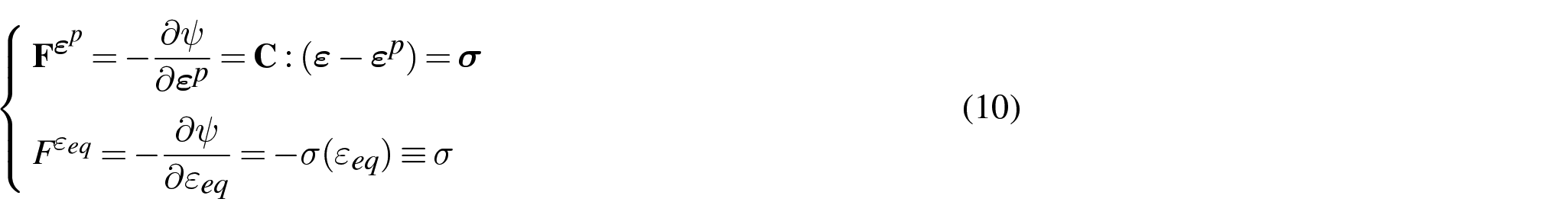
(by definition of the current yield stress $\bar{σ}$ ). In addition, the derivative of ψ with respect to ε gives σ , as required. Indeed, we have $\frac{\partial ψ}{\partial ε} = C : (ε - ε^{p}) = σ$ . The thermodynamic forces associated with the internal variable $ε^{p}$ are given by $F \equiv - \frac{\partial ψ}{\partial ε^{p}} = C : (ε - ε^{p}) - c ε^{p} = σ - α$ , $α = c ε^{p}$ , as also desired.

The next task to complete is to check that the reversibility domain defined by von Mises yield criterion with isotropic hardening in the space of thermodynamic forces (by expressing von Mises yield function as a function of the variables $F^{ε^{p}}$ and $F^{ε_{eq}}$ , instead of the variables σ and σ) is convex. The transformation of the variables ( σ , σ) to ( $F^{ε^{p}}$ , $F^{ε_{eq}}$ ) = ( $σ, - σ$ ) being linear, it suffices to show that the reversibility domain in the space of the first variables, $C \equiv {(σ, σ); Φ (σ, σ) \leq 0}$ , is convex. This is obvious due to the fact that von Mises yield function Φ² is a convex function with respect to the global variable ( σ , σ). Indeed,

Φ (σ, \bar{σ}) = Φ (F^{ε^{p}}, F^{ε_{eq}}) = σ_{eq} - \bar{σ} = ‖ F^{{ε^{p}}^{'}} ‖ + F^{ε_{eq}}

(11)

where the symbol $‖ . ‖$ denotes the Eucludian norm. It follows that von Mises yield function Φ is convex; hence, by the linearity of the transformation of the variables ( σ , $\bar{σ}$ ) to ( $F^{ε^{p}}$ , $F^{ε_{eq}}$ )=( $σ, - \bar{σ}$ ), the reversibility domain is convex with respect to the global variable ( σ , $\bar{σ}$ ).

The last thing to check is that the evolution equations associated to the internal variables $ε^{p}$ and $ε_{eq}$ satisfy the “generalized normality rule” with respect to the von Mises yield function, expressed as a function of the thermodynamic forces, i.e.:

{\begin{matrix} {\dot{ε}}^{p} = η \frac{\partial Φ}{\partial F^{ε^{p}}} \equiv η \frac{\partial Φ}{\partial σ} \\ {\overset{\cdot}{ε}}_{eq} = η \frac{\partial Φ}{\partial F^{ε_{eq}}} \equiv - η \frac{\partial Φ}{\partial σ} \end{matrix}

(12)

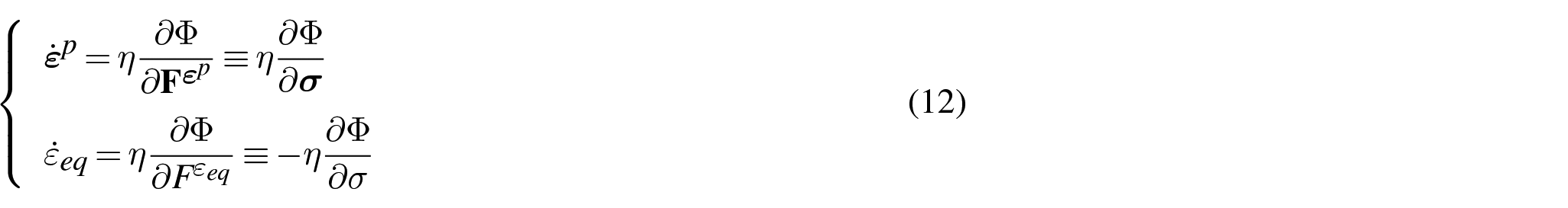
Note that the evolution equation (12)₁ is equivalent to the flow rule associated with the yield criterion by the normality property. It suffices, to complete the verification, to check that the evolution equation (12)₂ is satisfied. And yet

Φ (σ, σ) = σ_{eq} - σ \Rightarrow \frac{\partial Φ}{\partial σ_{ij}} = \frac{3}{2} \frac{{σ_{ij}}^{'}}{σ_{eq}} and \frac{\partial Φ}{\partial σ} = - 1 .

The relation (12)₁ then gives

{\overset{\cdot}{ε}}_{ij}^{p} = η \frac{3}{2} \frac{σ_{ij}^{'}}{σ_{eq}} .

(13)

Taking the magnitude of both sides of equation (13), we get

η = {\overset{\cdot}{ε}}_{eq},

which is precisely the value of η given by equation (12)₂. Hence, the “generalized normality rule” with respect to the global variable $(ε, ε_{eq})$ is satisfied. This proves that the small strain von Mises plasticity model with isotropic hardening can be described within the context of generalized standard materials, which guarantees that this model is automatically thermodynically consistent. From the numerical point of view, the generalized standard character of von Mises model ensures that the tangent matrix associated with the global elasto-plastic iterations is symmetric; this should avoid spurious problems of non-invertible matrix arising during nonlinear analyses. The property also warrants that the problem of projection of the elastically computed stress tensor onto the yield locus (plastic correction of the elastic predictor) admits a unique solution, provided that the equations of this problem are obtained through implicit time-discretization with respect to the components of the plastic strain and the hardening parameter.

3.2. Implications in terms of numerical implementation of the von Mises Model into a finite-element code

3.2.1. Description of the algorithm

The implementation of the global step may introduce complexities; however, this is not a concern when integrating a new plasticity model into a computational code, as the global step is entirely independent of the discretization (mesh) used. The primary focus should be on the local step, which requires careful attention. Specifically, only the material points (integration points) where the elastic and plastic strain increments, as well as the associated stress and strain tensors, are computed will be considered.

In practice, all Gauss points across the structure are processed sequentially, but this is handled automatically by the software, so there is no need for concern. The emphasis will remain on the local step. Quantities denoted by $(0)$ correspond to time t, while those without indices represent time $t + Δ t$ . Known quantities include $σ^{(0)}$ , $ε_{eq}^{(0)}$ , and $Δ ε$ (the total strain increment between time t and $t + Δ t$ ). The uniform application of the following formula is then carried out

σ^{*} = σ^{(0)} + λ (tr (Δ ε)) I + 2 μ Δ ε

where $σ^{*}$ is called the ”elastically computed stress” or ”elastic predictor”; it represents the final value of the stress, assuming that the total strain increment is purely elastic.

There are several technical reasons for considering $σ^{★}$ instead of handling $σ^{0}$ and $Δ ε$ separately. One key reason is that in the absence of plastic deformation between times t and $t + Δ t$ , the final stress σ simply equals $σ^{★}$ .

(Note that if plasticity is involved, $σ^{★}$ will not converge to σ at the end of the iterative process, as $σ^{★}$ represents the stress assuming purely elastic behavior, which is not applicable in the presence of plasticity.)

The task is to compute the elastic and plastic strain increments $(Δ ε^{e} + Δ ε^{p})$ , the equivalent strain increment $Δ ε_{eq}$ , and the final stress. We first employ the elasticity constitutive law:

ε^{e} = \frac{1 + ν}{E} σ - \frac{ν}{E} (tr (σ)) I

and the assumption of the additivity of the deformation.

\begin{matrix} σ = σ^{(0)} + λ (tr (Δ ε^{e})) I + 2 μ Δ ε^{e} \\ = σ^{(0)} + λ (tr (Δ ε - Δ ε^{p})) I + 2 μ (Δ ε - Δ ε^{p}) \\ = σ^{(0)} + λ (tr (Δ ε)) I + 2 μ Δ ε - (λ tr (Δ ε^{p}) I + 2 μ Δ ε^{p}) \\ = σ^{(0)} + λ (tr (Δ ε)) I + 2 μ Δ ε - 2 μ Δ ε^{p} \\ = σ^{★} - 2 μ Δ ε^{p} \end{matrix}

(14)

The term $2 μ Δ ε^{p}$ is referred to as the ”plastic correction.” This correction is applied to the elastic predictor to obtain the final stress value.

Second, the plastic flow rule will be used, discretized with an implicit scheme (note that $σ_{eq}$ and s are evaluated at time $t + Δ t$ ):

\begin{matrix} Δ ε^{p} = \frac{3}{2} (\frac{Δ ε_{eq}}{σ_{eq}}) s; \\ Δ ε_{eq} = \frac{2}{3} (Δ ε_{ij}^{p} Δ ε_{ij}^{p}) \end{matrix}

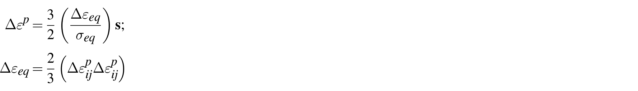
The last equation represents one of the von Mises criteria, evaluated at time $t + Δ t$ .

σ_{eq} = σ_{y} (ε_{eq}) = σ_{y} (ε_{eq}^{(0)} + Δ ε_{eq}) = σ_{y} (ε_{eq}^{(0)}) + h Δ ε_{eq}

in other words,

σ_{y} (ε_{eq}^{(0)} + Δ ε_{eq}) = σ_{y} (ε_{eq}^{(0)}) + σ_{y} (Δ ε_{eq})

The equations for this phase to consider are therefore as follows:

S : {\begin{matrix} σ & = σ^{★} - 2 μ Δ ε^{p} \\ Δ ε^{p} & = \frac{3}{2} \frac{Δ ε_{eq}}{σ_{eq}} s \\ σ_{eq} & = σ_{y} (ε_{eq}^{(0)}) + h Δ ε_{eq} \end{matrix}

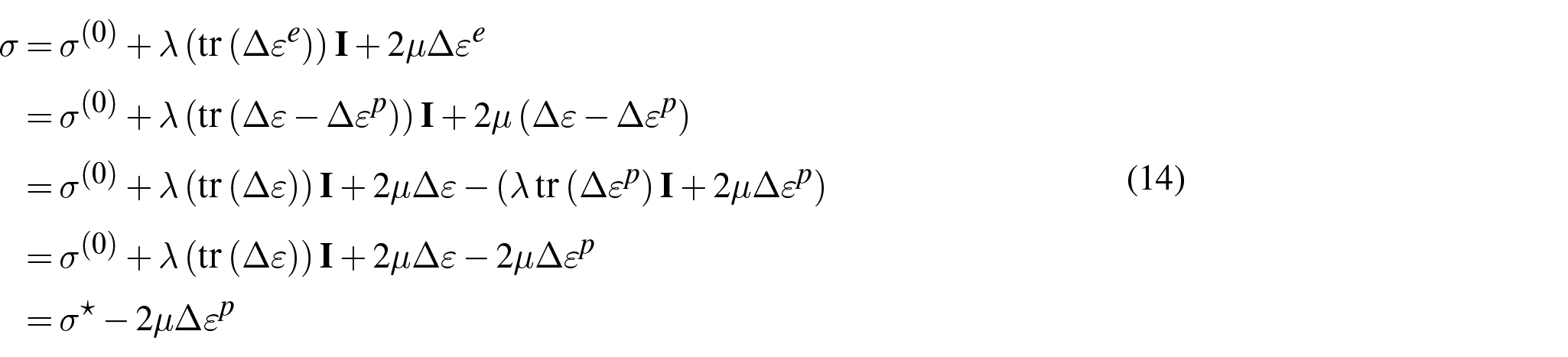
Of course, the previous equations help to better understand the meaning of this section. The algorithm is implicit due to $Δ ε^{p} = \frac{3}{2} \frac{Δ ε_{eq}}{σ_{eq}} s$ , which involves an implicit scheme.

The elastically computed stresses, denoted as $σ^{★}$ , are projected onto the von Mises criterion. Specifically, the final stresses σ are derived from the elastically computed stresses $σ^{★}$ by subtracting $2 μ Δ ε^{p}$ , which is collinear with σ and thus orthogonal to the yield surface defined by the von Mises criterion at the stress point σ .

Let us now solve the system $(S)$ . By differentiating the first equation of the system and combining it with the second equation, we obtain:

\begin{matrix} s = s^{★} - 2 μ Δ ε^{p} \\ = s^{★} - 2 μ (\frac{3}{2} \frac{Δ ε_{eq}}{σ_{eq}}) s \\ = s^{★} - 3 μ \frac{Δ ε_{eq}}{σ_{eq}} s \Rightarrow s^{★} = (1 + 3 μ \frac{Δ ε_{eq}}{σ_{eq}}) s \end{matrix}

where s represents the derivative of the elastically computed stress tensor. The equation illustrates a fundamental characteristic of the implicit algorithm and its projection onto the criterion: the derivative of the final stress tensor is positively collinear with σ . This property significantly simplifies the solution process, as it reduces the problem to iteratively solving a scalar equation for the unknown $Δ ε_{eq}$ . This simplification is not generally available with other types of plasticity criteria, nor with explicit algorithmic approaches.

For example, if we were to explicitly write out the time discretization of the flow rule (i.e., using an explicit scheme for the time discretization of the flow rule), we would have

Δ ε^{p} = \frac{3}{2} \frac{Δ ε_{eq}}{σ_{eq}^{(0)}} s^{(0)}

which would have implied

s = s^{★} - 3 μ \frac{Δ ε_{eq}}{σ_{eq}^{(0)}} s^{(0)}

and we would have lost the collinearity of s and $s^{★}$ .

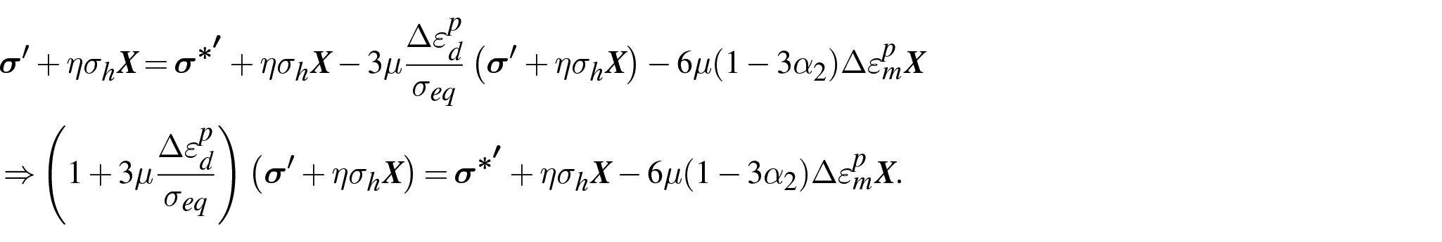
Taking the von Mises norm of the expression $s^{★} = (μ + 3 μ \frac{Δ ε_{eq}}{σ_{eq}}) s$ , we get

\begin{matrix} {(\frac{3}{2})}^{1 / 2} {(s^{★} : s^{★})}^{1 / 2} = (1 + 3 μ \frac{Δ ε_{eq}}{σ_{eq}}) {(\frac{3}{2} s_{ij} s_{ij})}^{1 / 2} \\ σ_{eq}^{★} = (1 + 3 μ \frac{Δ ε_{eq}}{σ_{eq}}) σ_{eq} \\ = σ_{eq} + 3 μ Δ ε_{eq} . \end{matrix}

Using the expression:

σ_{eq} = σ_{y} (ε_{eq}^{(0)}) + h Δ ε_{eq}

we get

\begin{matrix} σ_{eq}^{★} = σ_{y} (ε_{eq}^{(0)}) + h Δ ε_{eq} + 3 μ Δ ε_{eq} \\ = σ_{eq} (ε_{eq}^{(0)}) + (h + 3 μ) Δ ε_{eq} \end{matrix}

which implies that

Δ ε_{eq} = \frac{σ_{eq}^{★} - σ_{eq} (ε_{eq}^{(0)})}{h + 3 μ} .

When $Δ ε_{eq}$ is known, $ε_{eq}$ is immediately incremented as:

ε_{eq} = ε_{eq}^{(0)} + Δ ε_{eq} .

Similarly $Δ ε^{p}$ is given by

\begin{matrix} Δ ε^{p} = \frac{3}{2} \frac{Δ ε_{eq}}{σ_{eq}} s \\ s^{★} = (1 + 3 μ \frac{Δ ε_{eq}}{σ_{eq}}) s \end{matrix}

which implies

s = (\frac{1}{1 + 3 μ \frac{Δ ε_{eq}}{σ_{eq}}}) s^{★} .

From there we have

Δ ε^{p} = \frac{3}{2} \frac{Δ ε_{eq}}{σ_{eq}^{★}} s^{★} .

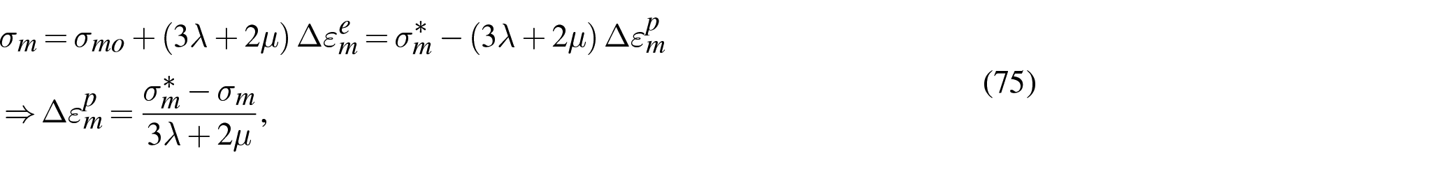
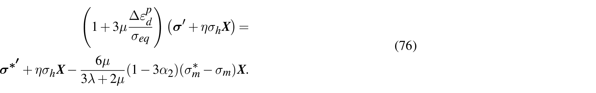
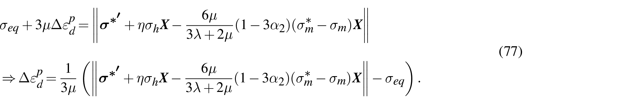
From the equation

σ = σ^{★} - 2 μ Δ ε^{p}

(15)

we deduce the value of σ .

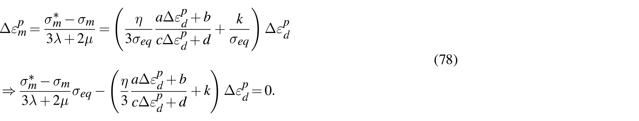
In fact, the preceding analysis only accounts for the scenario where plasticity occurs within the interval $[t, t + Δ t]$ . This happens when the equivalent stress is slightly below the threshold $(σ_{eq}^{★} - σ_{y}^{(0)})$ .

More precisely, this implies that the equivalent stress at $[t, t + Δ t]$ , computed under the assumption of purely elastic behavior, exceeds the yield strength for the current value of the accumulated strain $ε_{eq}^{(0)}$ .

There may be cases where the stress is marginally below the threshold $tr \leq 0$ , indicating the absence of plastic deformation between t and $t + Δ t$

In such situations, we impose $(Δ ε_{eq} = 0; ε_{eq} = ε_{eq}^{(0)} and σ = σ^{★}) .$

Thus, it follows that $Δ ε_{eq} = 0$ , $ε_{eq} = ε_{eq}^{(0)}$ and $σ = σ^{★}$ .

It is important to note that the algorithm remains agnostic as to whether the material exhibits plastic behavior at time t. Indeed, it only evaluates the von Mises yield criterion at $t + Δ t$ , rather than at the initial time t.

The algorithm is applied without modification, even if the material is elastic at time t and becomes plastic at time $t + Δ t$ , such that $t^{'} \in [t, t + Δ t]$ .

3.3. Implications on the numerical implementation into a finite-element code

As established in Section 4, the von Mises model characterizes a generalized standard material, incorporating plastic strain as an internal state variable. This formulation guarantees the existence and uniqueness of the solution to the associated projection problem, provided the evolution equations governing plastic strain is temporally discretized using an implicit integration scheme. However, the analysis presented in Section 4 is restricted to the context of a linearized kinematic framework, which can be overly simplistic for plasticity simulations involving large deformations. By extending the approach of Enakoutsa et al. [7], it is possible to remove the limitations imposed by the linearized theory, allowing for the investigation of how large deformation gradients, including both displacements and strains, affect the numerical stability and accuracy of the implementation:

At time step $t + Δ t$ , the equilibrium equations must be solved by updating the configuration of the geometry at this instant. This update is performed exclusively at the beginning of each outer elasto-plastic iteration, ensuring that the geometry remains fixed during the resolution of the subsequent projection problem. As a result, the projection problem is formulated with a frozen geometry, ensuring that the mathematical properties, such as existence, uniqueness, and stability of the solution, remain invariant under the geometric update at $t + Δ t$

For large strains and displacements, the classical elasticity law must be replaced by a hypoelastic formulation, utilizing an objective stress rate such as the Jaumann derivative. This objective derivative accounts not only for the conventional material time derivative but also incorporates non-trivial contributions involving the Cauchy stress tensor, the deformation gradient, and the velocity gradient. As demonstrated by Enakoutsa et al. [7], discretizing these additional terms using an explicit time-stepping scheme introduces known quantities that remain fixed throughout each global elasto-plastic iteration. These terms effectively serve as corrective modifications to the elastic stress predictor and do not impact the mathematical properties, such as the existence or uniqueness, of the local projection problem.

3.4. Uniqueness of the return mapping solution

To prove the uniqueness of the solution in the return mapping algorithm, we rely on the following points:

3.4.1. Convexity of the return map

The plastic potential $f (σ, σ_{Y})$ is convex meaning that when the trial stress violates the yield condition, there is a unique way for the stress state to return to the yield surface. This ensures that the stress correction $σ (t + Δ t)$ is unique.

3.4.2. Monotonicity of the hardening law

The isotropic hardening law $σ (ε_{eq})$ is monotonic, meaning that the yield stress always increases with increasing plastic strain (or remains constant in the case of perfect plasticity). This prevents oscillations or multiple solutions for the updated yield stress and plastic strain.

3.4.3. Positive definite tangent modulus

In the Newton–Raphson iterative scheme used to solve the nonlinear system in the return mapping algorithm, the key quantity is the consistent tangent modulus, which governs how the stress and plastic strain are updated at each iteration. For von Mises plasticity, the consistent tangent operator is positive definite, meaning that the Newton–Raphson iterations will always converge to a unique solution.

The consistent tangent modulus is derived from the stress–strain relationship and the plastic flow rule. It takes the form:

C_{\tan} = C - \frac{(C : n) \otimes (C : n)}{n : C : n + h}

(16)

where n is the normal to the yield surface, and h is the hardening modulus.

Since C (the elastic stiffness tensor) is positive definite and $h \geq 0$ (for isotropic hardening), the consistent tangent modulus remains positive definite, ensuring that the return mapping algorithm converges to a unique solution.

3.4.4. Existence of the solution

The return mapping algorithm ensures the existence of a solution by construction. The trial stress state is always projected back onto the yield surface in the direction of plastic flow, meaning that a solution always exists for the updated stress and plastic strain at each time increment.

In conclusion, by leveraging the convexity of the yield function, the positive definiteness of the tangent modulus, and the monotonicity of the hardening law, the return mapping algorithm for von Mises plasticity with isotropic hardening is guaranteed to have a unique solution. The iterative process used in the return mapping algorithm converges reliably due to these properties, ensuring that the stress and plastic strain are updated in a well-posed and physically consistent manner at each time step.

4. Example 02: GLD model and the class of GSM

4.1. Governing equations of the GLD model

In the model proposed by Gologanu et al. [9], the cavities are assumed to be ellipsoidal and axisymmetric, and aligned in the third direction of the cartesian system of coordinates ( $e_{1}$ , $e_{2}$ , $e_{3}$ ). The porosity f is defined as the ratio of the cavities volume to the total volume of the matter and the cavities. The shape factor of cavities is defined as the logarithm of the ratio of the axis of a cavity in the direction $e_{3}$ and a perpendicular direction.

Just like the majority of classical plasticity models in large deformation, the GLD model introduces an assumption of additive decomposition of the Eulerian strain rate into elastic and plastic parts, $ε \equiv ε^{e} + ε^{p}$ , and a hypoelasticity law connecting the elastic strain rate $ε^{e}$ to some objective time-derivative of the Cauchy stress tensor σ . We shall not insist on these standard features but focus on the new elements of the model, which are defined below.

4.1.1. Yield criterion

The yield criterion is given by the relation

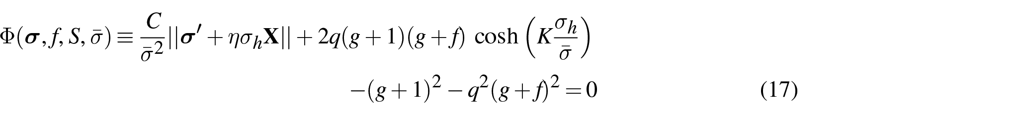
\begin{matrix} Φ (σ, f, S, \bar{σ}) \equiv \frac{C}{{\bar{σ}}^{2}} ‖ σ^{'} + η σ_{h} X ‖ + 2 q (g + 1) (g + f) \cosh (K \frac{σ_{h}}{\bar{σ}}) \\ - {(g + 1)}^{2} - q^{2} {(g + f)}^{2} = 0 \end{matrix}

(17)

where

σ ′ represents the deviatoric part of the stress tensor σ ;

X is the tensor defined as

X = \frac{1}{3} (- e_{1} \otimes e_{1} - e_{2} \otimes e_{2} + 2 e_{3} \otimes e_{3})

(18)

(the unit vector $e_{3}$ is parallel to the axis of the cavities);

‖·‖ is the von Mises magnitude symbol given by

‖ T ‖ \equiv {(\frac{3}{2} T^{'} : T^{'})}^{1 / 2}

(19)

(we shall adopt in the subsequent simplified notation

σ_{eq} = ‖ σ^{'} + η σ_{h} X ‖)

(20)

$\bar{σ}$ represents some average value of the yield stress in the heterogeneous metallic matrix;

C, η, K, g are the GLPD model parameters that depend on the porosity f and the shape factor of the cavities S; their expressions can be found by Gologanu et al. [9] and are not repeated here;

the stress $σ_{h}$ is defined as:

σ_{h} = α_{2} (σ_{11} + σ_{22}) + (1 - 2 α_{2}) σ_{33}

(21)

where $α_{2}$ is a parameter depending on the porosity f and the shape factor of the cavities S;

finally, q is the Tvergaard [10] parameter.

4.1.2. Evolution equations of the internal variables

The evolution equation for the porosity, calculated from the approximate incompressibility (the elasticity being neglected) assumption of the sane matrix material, is given by

\overset{\cdot}{f} \equiv 3 (1 - f) {\overset{\cdot}{ε}}_{m}^{p} + A {\overset{\cdot}{ε}}_{eq}

(22)

with ${\overset{\cdot}{ε}}_{m}^{p} = 1 / 3 tr {\overset{\cdot}{ϵ}}^{p}$ denoting the mean part of the plastic deformation rate ${\overset{\cdot}{ϵ}}^{p}$ , ${\overset{\cdot}{ε}}_{eq}$ , the equivalent plastic strain rate, and A, a model parameter connected to cavities nucleation.

The rate of the shape factor of the cavities is defined as

\overset{\cdot}{S} = \frac{3}{2} h {\overset{\cdot}{ε}}_{33}^{p^{'}} + 3 (\frac{1 - 3 α_{1}}{f} + 3 α_{2} - 1) {\overset{\cdot}{ε}}_{m}^{p}

(23)

where ${\overset{\cdot}{e}}^{p^{'}}$ denotes the deviatoric part of the plastic deformation rate ${\overset{\cdot}{e}}^{p}$ , ${\overset{\cdot}{ε}}_{m}^{p} = \frac{1}{3} tr ({\overset{\cdot}{e}}^{p})$ is its mean part, and $α_{1}$ is a parameter that is a function of the porosity f and the shape factor of the cavities S. Finally, h is a parameter which depends on the porosity f, the shape factor of the cavities, in addition to the triaxiality T defined by:

T = \frac{σ_{m}}{‖ σ^{'} ‖}, σ_{m} = \frac{1}{3} tr σ .

(24)

The variable $\bar{σ}$ is given by

\bar{σ} \equiv σ (\bar{ϵ})

(25)

where $σ (ϵ)$ is the function giving the yield limit as a function of the equivalent cumulated plastic strain ϵ, and $\bar{ϵ}$ denotes the average value of this equivalent strain in the heterogeneous matrix. The evolution equation of $\bar{ϵ}$ obeys the following law:

(1 - f) \bar{σ} \dot{\bar{ϵ}} = σ : ϵ^{p},

(26)

following an earlier suggestion of Gurson. Finally, the rate of change of the vector $e_{3}$ parallel to the axis of the cavities is defined as

{\overset{\cdot}{e}}_{3} = Ω e_{3}

(27)

where Ω is the rotation rate of the matter (for example the skew-symmetric part of the velocity gradient).

4.1.3. Flow rule

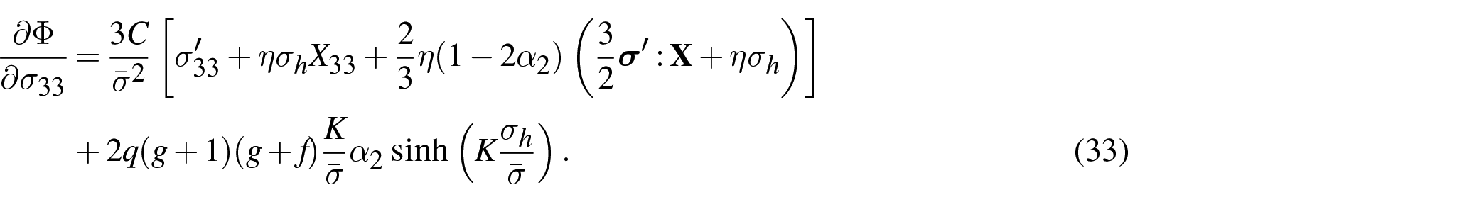
The plastic part of the additive decomposition of the deformation, deduced from the normality property, is obtained as

{\overset{\cdot}{ϵ}}^{p} = λ \frac{\partial Φ}{\partial σ}, λ \geq 0

(28)

where Φ denotes the GLP yield function (see equation (17)) and λ is the plastic multiplier. We shall now derive the explicit expressions of the plastic flow rule, equation (28). To that end, we begin by calculating the derivative

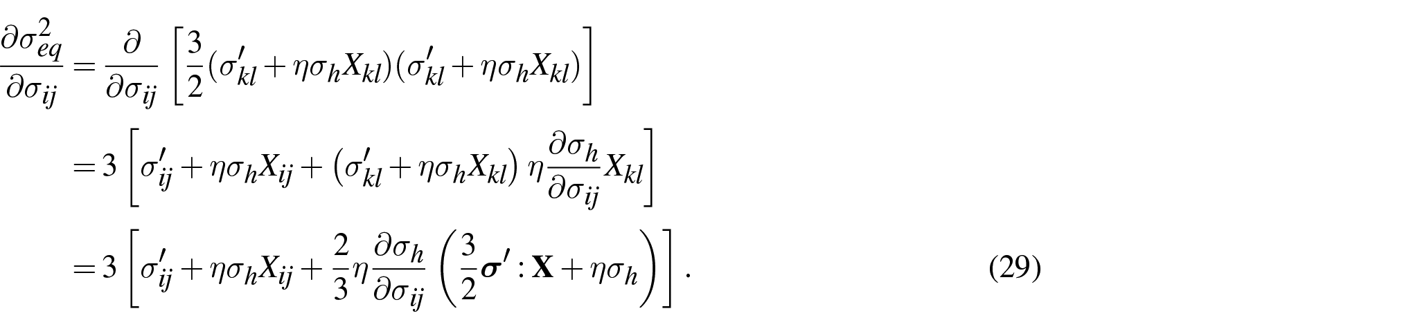
\begin{matrix} \frac{\partial σ_{eq}^{2}}{\partial σ_{ij}} = \frac{\partial}{\partial σ_{ij}} [\frac{3}{2} (σ_{kl}^{'} + η σ_{h} X_{kl}) (σ_{kl}^{'} + η σ_{h} X_{kl})] \\ = 3 [σ_{ij}^{'} + η σ_{h} X_{ij} + (σ_{kl}^{'} + η σ_{h} X_{kl}) η \frac{\partial σ_{h}}{\partial σ_{ij}} X_{kl}] \\ = 3 [σ_{ij}^{'} + η σ_{h} X_{ij} + \frac{2}{3} η \frac{\partial σ_{h}}{\partial σ_{ij}} (\frac{3}{2} σ^{'} : X + η σ_{h})] . \end{matrix}

(29)

Assuming that the Greek indices take only the values 1 and 2 and accounting for the following relations

\frac{\partial σ_{h}}{\partial σ_{α β}} = α_{2} δ_{α β}, \frac{\partial σ_{h}}{\partial σ_{α 3}} = 0, \frac{\partial σ_{h}}{\partial σ_{33}} = 1 - 2 α_{2},

(30)

\begin{matrix} \frac{\partial Φ}{\partial σ_{α β}} = \frac{3 C}{{\bar{σ}}^{2}} [σ_{α β}^{'} + η σ_{h} X_{α β} + \frac{2}{3} η (1 - 2 α_{2}) (\frac{3}{2} σ^{'} : X + η σ_{h})] \\ + 2 q (g + 1) (g + f) \frac{K}{\bar{σ}} (1 - 2 α_{2}) \sinh (K \frac{σ_{h}}{\bar{σ}}), \end{matrix}

(31)

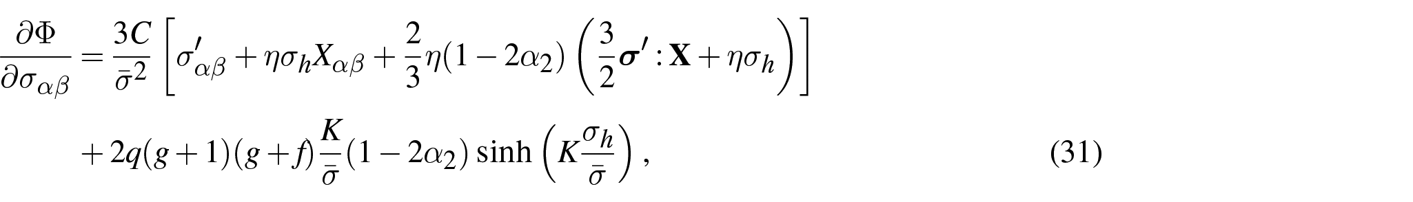
and

\frac{\partial Φ}{\partial σ_{α 3}} = \frac{C}{{\bar{σ}}^{2}} σ_{α 3}

(32)

we obtain

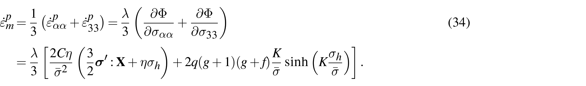
\begin{matrix} \frac{\partial Φ}{\partial σ_{33}} = \frac{3 C}{{\bar{σ}}^{2}} [σ_{33}^{'} + η σ_{h} X_{33} + \frac{2}{3} η (1 - 2 α_{2}) (\frac{3}{2} σ^{'} : X + η σ_{h})] \\ + 2 q (g + 1) (g + f) \frac{K}{\bar{σ}} α_{2} \sinh (K \frac{σ_{h}}{\bar{σ}}) . \end{matrix}

(33)

We can then compute the mean part of the plastic deformation rate ${\overset{\cdot}{ϵ}}^{p}$ as

\begin{matrix} {\overset{\cdot}{ε}}_{m}^{p} = \frac{1}{3} ({\overset{\cdot}{ε}}_{α α}^{p} + {\overset{\cdot}{ε}}_{33}^{p}) = \frac{λ}{3} (\frac{\partial Φ}{\partial σ_{α α}} + \frac{\partial Φ}{\partial σ_{33}}) \\ = \frac{λ}{3} [\frac{2 C η}{{\bar{σ}}^{2}} (\frac{3}{2} σ^{'} : X + η σ_{h}) + 2 q (g + 1) (g + f) \frac{K}{\bar{σ}} \sinh (K \frac{σ_{h}}{\bar{σ}})] . \end{matrix}

(34)

Also, combining the relations (28), (33), and (34), we get

{\begin{matrix} {\overset{\cdot}{ε}}_{α β}^{p} = λ \frac{3 C}{{\bar{σ}}^{2}} (σ_{α β}^{'} + η σ_{h} X_{α β}) + 3 α_{2} δ_{α β} {\overset{\cdot}{ε}}_{m}^{p} \\ {\overset{\cdot}{ε}}_{α 3}^{p} = λ \frac{3 C}{{\bar{σ}}^{2}} σ_{α 3} \\ {\overset{\cdot}{ε}}_{33}^{p} = λ \frac{3 C}{{\bar{σ}}^{2}} (σ_{33}^{'} + η σ_{h} X_{33}) + 3 (1 - 2 α_{2}) {\overset{\cdot}{ε}}_{m}^{p} . \end{matrix}

(35)

In the subsequent, let assume that

{\overset{\cdot}{ϵ}}_{d}^{p} = {\overset{\cdot}{ϵ}}^{p} - 3 α_{2} {\overset{\cdot}{ε}}_{m}^{p} e_{α} \otimes e_{α} - 3 (1 - α_{2}) {\overset{\cdot}{ε}}_{m}^{p} e_{3} \otimes e_{3} .

(36)

(Note that ${\overset{\cdot}{ϵ}}_{d}^{p}$ is a purely deviatoric tensor, i.e. $tr {\overset{\cdot}{ϵ}}_{d}^{p} = 0$ ). Combining the relations (35) and (36) we get

{\overset{\cdot}{ϵ}}_{d}^{p} = λ \frac{3 C}{{\bar{σ}}^{2}} (σ^{'} + η σ_{h} X) .

(37)

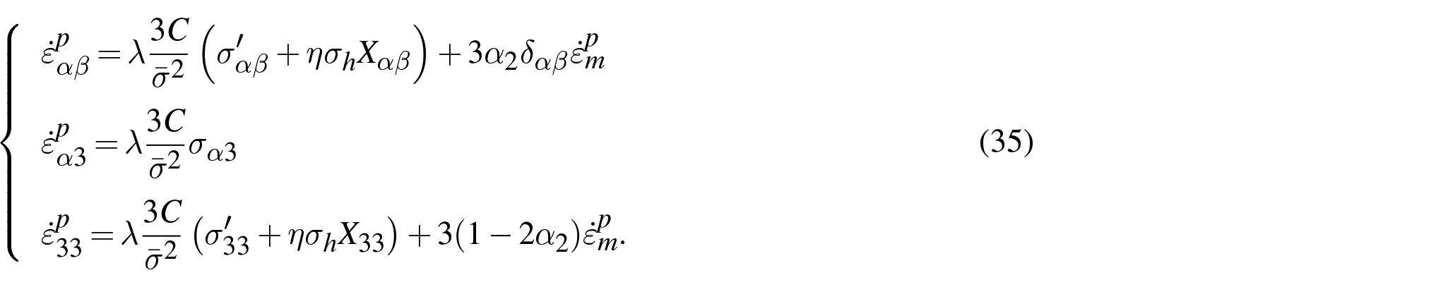
Thus, the tensors ${\overset{\cdot}{ϵ}}_{d}^{p}$ and $σ^{'} + η σ_{h} X$ are positively collinear. It follows that

{\overset{\cdot}{ϵ}}_{d}^{p} = \frac{3}{2} \frac{{\overset{\cdot}{ε}}_{d}^{p}}{σ_{eq}} (σ^{'} + η σ_{h} X),

(38)

with

{\overset{\cdot}{ε}}_{d}^{p} = {(\frac{2}{3} {\overset{\cdot}{ϵ}}_{d}^{p} : {\overset{\cdot}{ϵ}}_{d}^{p})}^{2}

(39)

( ${\overset{\cdot}{ε}}_{d}^{p}$ is equal to 2/3 of the von Mises norm of ${\overset{\cdot}{ϵ}}_{d}^{p}$ ) and $σ_{eq}$ is given by equation (21). Furthermore, we get

λ = \frac{1}{2 C} \frac{{\bar{σ}}^{2} {\overset{\cdot}{ε}}_{d}^{p}}{σ_{eq}};

(40)

adding this result to equation (34) yields

\frac{{\overset{\cdot}{ε}}_{m}^{p}}{{\overset{\cdot}{ε}}_{d}^{p}} = \frac{η}{3 σ_{eq}} (\frac{3}{2} σ^{'} : X + η σ_{h}) + 2 q (g + 1) (g + f) \frac{K}{3 C} \frac{\bar{σ}}{σ_{eq}} \sinh (K \frac{σ_{h}}{\bar{σ}}) .

To summarize, the explicit equation of the flow rule is given by the relations

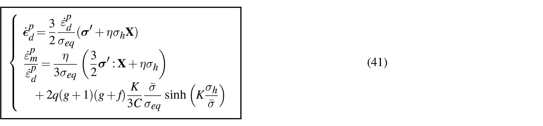
{\begin{array}{l} {\overset{\cdot}{ϵ}}_{d}^{p} = \frac{3}{2} \frac{{\overset{\cdot}{ε}}_{d}^{p}}{σ_{e q}} (σ^{'} + η σ_{h} X) \\ \frac{{\overset{\cdot}{ε}}_{m}^{p}}{{\overset{\cdot}{ε}}_{d}^{p}} = \frac{η}{3 σ_{e q}} (\frac{3}{2} σ^{'} : X + η σ_{h}) \\ + 2 q (g + 1) (g + f) \frac{K}{3 C} \frac{\bar{σ}}{σ_{e q}} \sinh (K \frac{σ_{h}}{\bar{σ}}) \end{array}

(41)

Note that in the case of a spherical cavity, $η = 0, C = 1, α_{2} = 0, g = 0$ , equation (41)₂ reduces the relation

\frac{{\overset{\cdot}{ε}}_{m}^{p}}{{\overset{\cdot}{ε}}_{d}^{p}} = 2 qf \frac{K}{3} \frac{\bar{σ}}{σ_{eq}} \sinh (K \frac{σ_{h}}{\bar{σ}}),

(42)

which corresponds to the theoretical equation of the flow rule for the Gurson model, see Gurson [11]. Remarkably, ${\overset{\cdot}{ε}}_{m}^{p}$ is non-zero in equation (42) since the porosity and the mean stress $σ_{h}$ are generally non-zero; thus, there is a plastic volume change of the cavity, which corresponds to an increase in the porosity for $σ_{h} > 0$ or a decrease of the porosity if $σ_{h} < 0$ . Hence, the model accounts very well for the growth and closure of cavities.

4.1.4. Parameterization of the yield surface

The numerical implementation of the GLD model requires solving the complex problem of projection of the elastic stress predictor onto the yield surface. One key point of the procedure of solution of the projection problem, aimed at reducing the number of unknowns, lies in a suitable parametrization of the yield locus defined by the yield function (17). This parametrization is inspired by the classical one for an ellipse and obtained by looking for the maximum possible value of the quantity $C \frac{σ_{eq}^{2}}{{\bar{σ}}^{2}}$ corresponding to $σ_{h} = 0$ , i.e. $(K \frac{σ_{h}}{\bar{σ}}) = 1$ . Using equation (17), we find

C \frac{σ_{eq}^{2}}{{\bar{σ}}^{2}} = {(g + 1)}^{2} + q^{2} {(g + f)}^{2} - 2 q (g + 1) (g + f) = [g + 1 - q (g + f)]^{2} .

(43)

Assuming that

C \frac{σ_{eq}^{2}}{{\bar{σ}}^{2}} = [g + 1 - q (g + f)]^{2} \cos^{2} (ϕ),

(44)

we obtain

σ_{eq} = \frac{\bar{σ}}{\sqrt{C}} [g + 1 - q (g + f)]^{2} \cos (ϕ)

(45)

where ϕ represents some angle with positive cosine. Hence, equation (17) yields

\begin{matrix} 2 q (g + 1) (g + f) \cosh (K \frac{σ_{h}}{\bar{σ}}) \\ = {(g + 1)}^{2} + q^{2} {(g + f)}^{2} - [g + 1 - q (f + g)]^{2} \cos^{2} (ϕ) \\ = 2 q (g + 1) (g + f) + [g + 1 - q (f + g)]^{2} \sin^{2} (ϕ) . \end{matrix}

(46)

Solving equation (46) for the parameter $σ_{h}$ we get

σ_{h} = \frac{\bar{σ}}{K} sgn (ϕ) \cosh^{- 1} (1 + \frac{{[g + 1 - q (g + f)]}^{2}}{2 q (g + 1) (g + f)} \sin^{2} (ϕ)) .

(47)

The sign of ϕ is introduced into equation (47) to allow for negative as well as positive values of $σ_{h}$ . Finally, the equations of the parametrization of the yield surface are given by

{\begin{array}{l} σ_{e q} = \frac{\bar{σ}}{\sqrt{C}} {[g + 1 - q (g + f)]}^{2} c o s (ϕ) \\ σ_{h} = \frac{\bar{σ}}{K} s g n (ϕ) \cosh^{- 1} (1 + \frac{{[g + 1 - q (g + f)]}^{2}}{2 q (g + 1) (g + f)} \sin^{2} (ϕ)) \end{array}

(48)

4.1.5. Nonlocal damage model based on the GLD model

The nonlocal damage model based on the Gologanu–Leblond–Devaux (GLD) model extends the classical [11] model by incorporating void shape evolution, which captures how voids elongate or flatten during plastic deformation, and a nonlocal treatment of damage, significantly improving the accuracy of simulations in ductile fracture, where the shape and distribution of voids play a critical role in material behavior.

Nonlocal approach

In traditional local damage models, damage evolution is computed at a specific material point based on local stress and strain states. However, a nonlocal damage model introduces spatial averaging, so the damage at any point also depends on the behavior of surrounding material points. This approach resolves issues like mesh sensitivity and unrealistic localization of damage.

Convolution of the evolution equation of the damage

The nonlocal aspect is introduced using a convolution operator, which spreads the effect of damage over a spatial domain. This convolution integrates the damage variable over neighboring points, ensuring that damage evolution considers both local and surrounding states. The mathematical representation of the convolution is given by:

\dot{\bar{f}} (x) = \int_{Ω} A (x, x^{'}) \overset{\cdot}{f} (x^{'}) d x^{'}

where $\dot{\bar{f}} (x)$ represents the nonlocal damage at point x, $\overset{\cdot}{f} (x^{'})$ is the local damage at a neighboring point $x^{'}$ , and $A (x, x^{'})$ is a weighting function (or kernel) that controls how much influence neighboring points have on the damage at x.

Mathematical formulation

The nonlocal GLD model replaces the local damage variable with a nonlocal one, introducing spatial averaging via the convolution operation. The mathematical form of the nonlocal damage variable is given by:

\dot{\bar{f}} (x) = \int_{Ω} A (x, x^{'}) \overset{\cdot}{f} (x^{'}) d x^{'}

where:

$\dot{\bar{f}} (x)$ is the nonlocal damage at point x,

$\overset{\cdot}{f} (x^{'})$ is the local damage at a neighboring point $x^{'}$ ,

$A (x, x^{'})$ is a weighting function that defines the influence of damage at point $x^{'}$ on point x,

Ω is the domain over which the convolution is computed.

The kernel function $A (x, x^{'})$ is chosen based on the material’s characteristic length scale and plays a crucial role in controlling the spatial distribution of damage. Theoretical Insights into Diffusion Analogy in Nonlocal Damage Models Nonlocal damage models, particularly those employing integral formulations, are known for their ability to mitigate mesh sensitivity in numerical simulations. However, these models often exhibit excessive smoothing, which is mathematically analogous to a diffusion process. This section formulates and proves two theorems that characterize the diffusive behavior of such models, providing a rigorous mathematical foundation for understanding their effects.

4.2. Excessive smoothing of the damage variable: theoretical results

Nonlocal damage models, particularly those employing integral formulations, are known for their ability to mitigate mesh sensitivity in numerical simulations. However, these models often exhibit excessive smoothing, which is mathematically analogous to a diffusion process. This section formulates and proves two theorems that characterize the diffusive behavior of such models, providing a rigorous mathematical foundation for understanding their effects. The first theorem establishes exponential attenuation of high-frequency components, while the second connects the nonlocal model to a diffusion-like equation. These insights are crucial for improving the design of nonlocal formulations to balance numerical stability and physical accuracy.

4.2.1. Attenuation of high-frequency components

Theorem 1. (Attenuation of high-frequency components). In the Fourier domain, the nonlocal damage model described by the convolution equation:

f (x, t) = \frac{1}{B (x)} \int_{Ω} A (x - y) f_{loc} (y, t) d V_{y},

with a Gaussian kernel $A (x - y) = \exp (- \frac{∥ x - y ∥^{2}}{l^{2}})$ , attenuates high-frequency components of the local damage $f_{loc}$ exponentially with a rate proportional to the square of the wavenumber p and the square of the kernel length scale l.

Proof. 1. Taking the Fourier transform of the convolution equation:

\hat{f} (p, t) = \hat{A} (p) {\hat{f}}_{loc} (p, t),

where $\hat{f} (p, t)$ and ${\hat{f}}_{loc} (p, t)$ are the Fourier transforms of the nonlocal and local damage, respectively, and $\hat{A} (p)$ is the Fourier transform of the Gaussian kernel:

\hat{A} (p) = \exp (- \frac{p^{2} l^{2}}{4}) .

2. The term $\hat{A} (p)$ acts as a multiplicative filter. For high wavenumbers p, the term $- \frac{p^{2} l^{2}}{4}$ dominates, leading to:

\hat{A} (p) \to \exp (- \frac{p^{2} l^{2}}{4}) as p \to \infty .

3. The exponential attenuation implies that:

| \hat{f} (p, t) | << | {\hat{f}}_{loc} (p, t) | for large p .

4. Therefore, high-frequency components (short-wavelength features) are exponentially suppressed, while low-frequency components remain relatively unaffected.

This completes the proof. □

4.2.2. Diffusion approximation of nonlocal damage

Theorem 2. (Diffusion Approximation). The nonlocal damage model:

f (x, t) = \frac{1}{B (x)} \int_{Ω} A (x - y) f_{loc} (y, t) d V_{y},

with a Gaussian kernel $A (x - y) = \exp (- \frac{∥ x - y ∥^{2}}{l^{2}})$ , is approximately governed by a diffusion-like equation:

f (x, t) \approx f_{loc} (x, t) - \frac{l^{2}}{4} \nabla^{2} f_{loc} (x, t),

where the term $\frac{l^{2}}{4} \nabla^{2} f_{loc} (x, t)$ represents the diffusive correction.

Proof. 1. Using the Fourier transform analysis, approximate the Gaussian kernel in the Fourier domain:

\hat{A} (p) = \exp (- \frac{p^{2} l^{2}}{4}) \approx 1 - \frac{p^{2} l^{2}}{4} + O (p^{4}),

for small p (long-wavelength components).

2. Substituting this into the Fourier-transformed equation for ϕ:

\hat{f} (p, t) \approx {\hat{f}}_{loc} (p, t) (1 - \frac{p^{2} l^{2}}{4}) .

3. Taking the inverse Fourier transform:

f (x, t) \approx f_{loc} (x, t) - \frac{l^{2}}{4} \nabla^{2} f_{loc} (x, t) .

4. The correction term $- \frac{l^{2}}{4} \nabla^{2} f_{loc} (x, t)$ introduces a diffusion-like behavior, where $\frac{l^{2}}{4}$ serves as the effective diffusion coefficient.

5. Therefore, the nonlocal model can be interpreted as a diffusive system where the Gaussian kernel introduces smoothing effects analogous to a diffusion process.

This completes the proof. □

4.3. Modified nonlocal evolution equation

4.3.1. Stability analysis of the modified nonlocal evolution equation

The excessive smoothing of damage in nonlocal models has long been a challenge in the numerical simulation of material behavior. This phenomenon, often attributed to the diffusive nature of the integral-type evolution equations, can lead to unrealistic results, such as delayed crack initiation and homogenized damage distributions near crack tips. To address this, a modified nonlocal evolution equation was proposed by Enakoutsa et al. [7], Enakoutsa [12], incorporating the logarithm of the damage variable. This section aims to rigorously analyze the stability of this revised formulation under small perturbations.

Mathematical formulation

The modified nonlocal evolution equation is given by:

\frac{d (\ln f)}{dt} (x) = \frac{1}{B (x)} \int_{Ω} A (x - y) {\frac{d (\ln f)}{dt}}_{loc} (y) d V_{y},

(49)

where $f (x, t)$ represents the damage variable, $A (x - y)$ is a Gaussian weighting kernel, and $B (x)$ is a normalization factor defined as:

B (x) = \int_{Ω} A (x - y) d V_{y} .

(50)

This formulation ensures that the damage evolution remains consistent across the domain while mitigating excessive smoothing.

Linearization

Let the damage variable $f (x, t)$ be perturbed around a steady-state solution $f_{0} (x)$ as:

f (x, t) = f_{0} (x) + δ f (x, t),

(51)

where $δ f (x, t)$ is a small perturbation. Taking the logarithm and expanding in a Taylor series:

\ln f (x, t) \approx \ln f_{0} (x) + \frac{δ f (x, t)}{f_{0} (x)} .

(52)

Substituting this into equation (49), we obtain the perturbation equation:

\frac{d (δ ψ (x, t))}{dt} = \frac{1}{B (x)} \int_{Ω} A (x - y) \frac{d (δ ψ (y, t))}{dt} d V_{y},

(53)

where $δ ψ (x, t) = \frac{δ f (x, t)}{f_{0} (x)}$ .

4.3.2. Fourier transform analysis

Applying the Fourier transform with respect to the spatial variable x:

\frac{\partial \hat{δ ψ} (p, t)}{\partial t} = \hat{A} (p) \frac{\partial \hat{δ ψ} (p, t)}{\partial t},

(54)

where $\hat{A} (p)$ is the Fourier transform of the Gaussian kernel $A (x - y)$ , given by:

\hat{A} (p) = \exp (- \frac{p^{2} l^{2}}{4}) .

(55)

Growth rate analysis

Rewriting the perturbation growth rate:

\frac{\partial \hat{δ ψ} (p, t)}{\partial t} (1 - \hat{A} (p)) = 0 .

(56)

For non-trivial solutions, stability requires $1 - \hat{A} (p) > 0$ , which holds for all $p \neq 0$ because $\hat{A} (p) < 1$ for $p \neq 0$ . The stability condition is therefore:

\sup_{p} | \hat{A} (p) | < 1 .

(57)

This analysis demonstrates that the modified nonlocal evolution equation avoids the excessive smoothing observed in the original formulation. The Gaussian kernel ensures that short-wavelength perturbations decay faster than long-wavelength ones, maintaining a realistic damage distribution.

Sensitivity Analysis of Length Scales in Nonlocal Damage Models Nonlocal damage models have gained prominence in computational mechanics due to their ability to address mesh sensitivity in simulations involving softening and localization phenomena. Central to these models is the length scale parameter l, which governs the extent of nonlocal interactions. While increasing l enhances regularization, it may also result in excessive smoothing, delaying the onset of localization and altering physical interpretations. This section investigates the impact of l on the model’s behavior, introducing a rigorous framework based on the second moment of the kernel to quantify the kernel’s spatial influence.

4.4. Effective smoothing radius and the second moment of a Kernel

The effective smoothing radius, $R_{eff}$ , quantifies the spatial extent of influence of the kernel function $A (x - y)$ . It is derived from the kernel’s second moment, defined as:

R_{eff}^{2} = \frac{\int_{Ω} ∥ x - y ∥^{2} A (x - y) d V_{y}}{\int_{Ω} A (x - y) d V_{y}} .

This definition includes:

Numerator: $\int_{Ω} ∥ x - y ∥^{2} A (x - y) d V_{y}$ , the weighted squared distance,

Denominator: $\int_{Ω} A (x - y) d V_{y}$ , the total volume of the kernel, ensuring normalization.

The second moment provides a rigorous and natural measure of the kernel’s spatial influence.

4.4.1. Application to the Gaussian Kernel

For the Gaussian kernel:

A (x - y) = \exp (- \frac{∥ x - y ∥^{2}}{l^{2}}),

we compute $R_{eff}$ as follows:

(a) Denominator: Total Volume

The total volume of the Gaussian kernel is:

\int_{Ω} A (x - y) d V_{y} = \int_{R^{d}} \exp (- \frac{∥ x - y ∥^{2}}{l^{2}}) d V_{y} = {(2 π)}^{d / 2} l^{d} .

(b) Numerator: Weighted Squared Distance

The numerator is:

\int_{Ω} ∥ x - y ∥^{2} A (x - y) d V_{y} = d \cdot \frac{l^{2}}{2} \cdot {(2 π)}^{d / 2} l^{d},

where d is the spatial dimensionality.

(c) Effective Radius

The effective smoothing radius is:

R_{eff} = \sqrt{\frac{\int_{Ω} ∥ x - y ∥^{2} A (x - y) d V_{y}}{\int_{Ω} A (x - y) d V_{y}}} = \sqrt{\frac{d \cdot l^{2}}{2}} .

In one-dimensional space ( $d = 1$ ):

R_{eff} = \frac{l}{\sqrt{2}} .

4.4.2. Sensitivity to Length Scale l

Critical length scale

A critical length scale $l_{c}$ is defined where high-frequency attenuation becomes significant. For a threshold wavenumber $p_{c}$ , the attenuation is:

\hat{A} (p_{c}) = \exp (- \frac{p_{c}^{2} l^{2}}{4}) \approx ϵ,

yielding:

l_{c} = \frac{2}{p_{c}} \sqrt{(\frac{1}{ϵ})} .

Impact on damage evolution

The length scale l also influences the diffusive correction term:

f (x, t) \approx f_{loc} (x, t) - \frac{l^{2}}{4} \nabla^{2} ϕ_{loc} (x, t) .

As l increases, the term $- \frac{l^{2}}{4} \nabla^{2} f_{loc} (x, t)$ becomes significant, leading to delayed damage localization and excessive smoothing.

A quick illustration

Consider a one-dimensional damage profile:

f_{loc} (x) = \exp (- x^{2}) .

The nonlocal damage profile $f (x)$ for various l is:

f (x) = \frac{1}{B (x)} \int_{- \infty}^{\infty} A (x - y) f_{l o c} (y) d y .

These results show that as l increases:

The damage profile broadens,

Peak damage values decrease,

Smoothing becomes more pronounced.

The effective smoothing radius $R_{eff}$ , derived from the second moment of the kernel, provides a rigorous measure of the kernel’s spatial influence. Analytical studies and examples reveal that increasing l enhances smoothing but may delay localization. Practical guidelines ensure an optimal balance between numerical stability and physical accuracy.

4.5. The GLD model and the class of generalized standard materials

In this section, we aim to examine the generalized standard nature of the GLP model under the assumption of small deformations. It should be noted that the formalism of generalized standard materials only applies under this assumption.

The examination demonstrates that, at a fixed porosity, the constitutive equations of the GLD model possess the required properties to ensure the model’s classification within the GSM class.

In the following section, we will explore the implications of this property concerning the numerical implementation of the model.

It is important to immediately note that this property applies equally to both the original local version of the model and its non-local modified version presented in Section 4, as fixing the porosity disregards its evolution equation, which is the only differing point between the two versions.

The presentation begins with a very brief general overview of some aspects of the work by Halphen and Nguyen [1], and Son [13] on the Generalized Strain Gradient (GSM). It continues by providing a simple example of MSG before delving into the main result of this section: the generalized standard nature of the GLP model when the porosity, the orientation, and the shape factor components in the model are assumed to be discretized with an explicit numerical scheme.

To begin with, it is necessary to define the state variables and the expression for the free energy, and then ensure that the latter satisfies the required properties (see Appendix 1).

The state of the material is described by the following state variables: the components of total deformation ε and a set of internal variables including the components of plastic deformation $ε^{p}$ and the cumulative equivalent plastic deformation.

We then propose the following free energy potential, which is the sum of elastic deformation energy and ”locked” hardening energy:

ψ (ε, ε^{p}, ε_{e q}) = \frac{1}{2} (ε - ε^{p}) : C : (ε - ε^{p}) + λ \int_{0}^{ε_{e q}} σ (ε) d ε .

(58)

In this equation, C represents the fourth-order elastic stiffness tensor, and $σ (ε_{eq})$ is the yield stress in simple tension, a function of cumulative plastic deformation.

It is easy to see, with this definition, that the free energy ψ is strictly convex with respect to the internal variable ε, as the quadratic form defined by C is positive definite. The free energy is also strictly convex with respect to $ε^{p}$ for the same reason as mentioned earlier. It is also strictly convex with respect to the variable $ε_{eq}$ due to the positivity of the hardening slope. Furthermore, it is a sum of strictly convex functions of $ε^{p}$ and $ε_{eq}$ (with ε fixed). Therefore, the free energy is strictly convex with respect to the global internal variable $(ε^{p}, ε_{eq})$ , as desired.

Moreover, the derivative of ψ with respect to ε is equal to σ , as desired as well, and the thermodynamic forces $F^{ε^{p}}$ and $F^{ε_{eq}}$ associated with the internal variables $ε^{p}$ and $ε_{eq}$ are given by:

{\begin{matrix} F^{ε^{p}} = - \frac{\partial ψ}{\partial ε^{p}} = C : (ε - ε^{p}) = s \\ F^{ε_{eq}} = - \frac{\partial ψ}{\partial ε_{eq}} = - σ (ε_{eq}) \equiv σ \end{matrix}

(59)

The second thing to do is to demonstrate that the reversibility domain defined by GLD criterion in the space of thermodynamic forces (expressing GLD’s charge function Φ in terms of the variables $F^{ε^{p}}$ and $F^{\bar{ϵ}}$ instead of σ and $\bar{σ}$ ) is convex.

The transformation from the variables ( σ , $\bar{σ}$ ) to the variables ( $F^{ε^{p}}$ , $F^{\bar{ϵ}}$ ) = ( $σ, - λ \bar{σ}$ ) is, however, linear. Therefore, it will be sufficient to prove that the reversibility domain in the space of the first variables,

C \equiv (σ, \bar{σ}); Φ (σ, \bar{σ}, S, f) \leq 0,

is convex.

This would result immediately from the convexity of GLD’s charge function Φ with respect to the global internal variable ( σ , $\bar{σ}$ ), if this function were convex.

The second element consists of checking that the evolution equations of the internal variables $ε^{p}$ and $\bar{ϵ}$ comply with the generalized normality property with respect to the GLD’s yield function, expressed in terms of thermodynamic forces:

{\begin{matrix} {\overset{\cdot}{ε}}^{p} = η \frac{\partial Φ}{{\partial F}^{ε^{p}}} \equiv η \frac{\partial Φ}{\partial σ} \\ \dot{\bar{ϵ}} = η \frac{\partial Φ}{\partial F^{\bar{ε}}} \equiv - \frac{η}{λ} \frac{\partial Φ}{\partial \bar{σ}} \end{matrix}

(60)

The two previous elements of this proof were extensively discussed by Enakoutsa et al. [7] in the context of the Gurson’s [11] model, and for this reason will not be repeated here.

All the necessary conditions for the GLD model with fixed porosity and the shape factor of the cavities to define a generalized standard material are thus satisfied.

The essential point here is that the evolution equation of the hardening parameter $\bar{ϵ}$ is such that the internal variables $ε^{p}$ and $\bar{ϵ}$ collectively satisfy a certain normality law. This property does not appear to be extendable to the case where the evolution of porosity and the shape factor of the cavities are taken into account, because the right-hand sides of these equations bear no relation to the derivative of the criterion with respect to the porosity and the shape factor of the cavity.

4.5.1. Implications in terms of numerical implementation of the GLD model: numerical algorithm

Projection onto the yield surface

The key challenge in the numerical implementation of an elastoplastic model lies in accurately projecting onto the yield surface. Specifically, the task is as follows: given the outcome of a ”large elastoplastic iteration” (where elastic deformation is solved over the entire structure, considering initial plastic strains), which yields the total strain increment $\nabla \dot{ε}$ over the time step from t to $t + \nabla t$ , we must determine the decomposition of $\dot{ε}$ into its elastic $\overset{e}{ε}$ and plastic $\overset{p}{ε}$ components. This decomposition must satisfy the yield criterion at $t + \nabla t$ and the flow rule governing plastic behavior during the time step, ultimately leading to the updated stress at $t + \nabla t$ .

In the following, quantities without indices refer to their values at time $t + Δ t$ , while those with the subscript ’0’ correspond to their values at time t (representing known quantities).

Let us begin by defining a parametrization of the original Gurson criterion using an angle ϕ, following the approach of the original model. This ensures automatic satisfaction of the criterion. The flow rules will then provide an equation for ϕ, which can be solved numerically.

To find this parametrization, let us look for the maximum value of $C \frac{σ_{eq}^{2}}{{\bar{σ}}^{2}}$ corresponding to $σ_{h} = 0 \Rightarrow (K \frac{σ_{h}}{\bar{σ}}) = 1$ ; according to equation (17)

C \frac{σ_{eq}^{2}}{{\bar{σ}}^{2}} = {(g + 1)}^{2} + q^{2} {(g + f)}^{2} - 2 q (g + 1) (g + f) = [g + 1 - q (g + f)]^{2} .

It is therefore natural to assume that

\begin{matrix} C \frac{σ_{eq}^{2}}{{\bar{σ}}^{2}} = [g + 1 - q (g + f)]^{2} co s^{2} φ \\ \Rightarrow σ_{eq} = \frac{\bar{σ}}{\sqrt{C}} [g + 1 - q (g + f)] \cos φ \end{matrix}

(61)

where φ is some angle with positive cosine. We get from equation (17)

\begin{matrix} 2 q (g + 1) (g + f) \cosh (K \frac{σ_{h}}{\bar{σ}}) & = {(g + 1)}^{2} + q^{2} {(g + f)}^{2} - [g + 1 - q (g + f)]^{2} co s^{2} φ \\ = {(g + 1)}^{2} + q^{2} {(g + f)}^{2} - [g + 1 - q (g + f)]^{2} \\ + [g + 1 - q (g + f)]^{2} si n^{2} φ \\ = 2 q (g + 1) (g + f) + [g + 1 - q (g + f)]^{2} si n^{2} φ \end{matrix}

(62)

\begin{matrix} \Rightarrow \cosh (K \frac{σ_{h}}{\bar{σ}}) = 1 + \frac{{[g + 1 - q (g + f)]}^{2}}{2 q (g + 1) (g + f)} si n^{2} φ \end{matrix}

\begin{matrix} \Rightarrow σ_{h} = \frac{\bar{σ}}{K} sgn (φ) \cos h^{- 1} (1 + \frac{{[g + 1 - q (g + f)]}^{2}}{2 q (g + 1) (g + f)} si n^{2} φ) \end{matrix}

We introduce $sgn (ϕ)$ (the sign of ϕ) to ensure that $σ_{h}$ can assume both positive and negative values. Equations (61) and (62) provide the parametrization for the criterion we seek. The angle ϕ is considered within the interval $[- \frac{π}{2}, \frac{π}{2}]$ , which allows $\cos (ϕ)$ to cover all positive values or zero, and $sgn (ϕ)$ to assume values of $\pm 1$ . Before expressing the flow rule in its discretized form, we first need to establish the relationships between $σ_{h}$ and $σ_{m}$ , and between ${\overset{\cdot}{ε}}_{d}^{p}$ and ${\overset{\cdot}{ε}}^{p'}$ as:

\begin{matrix} σ_{h} = α_{2} σ_{α α} + (1 - 2 α_{2}) σ_{33} = \frac{1}{3} (σ_{α α} + σ_{33}) + (α_{2} - \frac{1}{3}) σ_{α α} + 2 (\frac{1}{3} - α_{2}) σ_{33} \\ = σ_{m} + (1 - 3 α_{2}) (- \frac{1}{3} σ_{α α} + \frac{2}{3} σ_{33}) \end{matrix}

which gives, from the definition equation (18) of the tensor X :

σ_{h} = σ_{m} + (1 - 3 α_{2}) σ^{'} : X .

(63)

In addition, from equation (36),

\begin{matrix} {\overset{\cdot}{ε}}_{d}^{p} & = {\overset{\cdot}{ε}}^{p} - 3 α_{2} {\overset{\cdot}{ε}}_{m}^{p} {\hat{e}}_{α} \otimes {\hat{e}}_{α} - 3 (1 - 2 α_{2}) {\overset{\cdot}{ε}}_{m}^{p} {\hat{e}}_{3} \otimes {\hat{e}}_{3} \\ = {\overset{\cdot}{ε}}^{p} - {\overset{\cdot}{ε}}_{m}^{p} {\hat{e}}_{α} \otimes {\hat{e}}_{α} - {\overset{\cdot}{ε}}_{m}^{p} {\hat{e}}_{3} \otimes {\hat{e}}_{3} + (1 - 2 α_{2}) {\overset{\cdot}{ε}}_{m}^{p} {\hat{e}}_{α} \otimes {\hat{e}}_{α} + 2 (3 α_{2} - 1) {\overset{\cdot}{ε}}_{m}^{p} {\hat{e}}_{3} \otimes {\hat{e}}_{3} \\ = {\overset{\cdot}{ε}}^{p} - 3 (1 - 3 α_{2}) {\overset{\cdot}{ε}}_{m}^{p} X . \end{matrix}

(64)

Let us now write the flow rule in discretized form. $Δ ε_{d}^{p}$ being related to $Δ ε^{p^{'}}$ par the relationship

Δ ε_{d}^{p} = Δ ε^{p^{'}} - 3 (1 - 3 α_{2}) Δ ε_{m}^{p} X

(65)

(which is the discretized equivalent form of equation (64), we get:

Δ ε_{d}^{p} = \frac{3}{2} \frac{Δ ε_{d}^{p}}{σ_{eq}} (σ^{'} + η σ_{h} X)

(66)

where

Δ ε_{d}^{p} = {(\frac{3}{2} Δ ε_{d}^{p} : Δ ε_{d}^{p})}^{1 / 2} .

(67)

Note that these equations correspond to an implicit algorithm with respect to all parameters except the porosity f. The symbol $\tilde{f}$ represents an explicit approximation of porosity on the half-interval $t + \frac{Δ t}{2}$ given by

\frac{Δ ε_{m}^{p}}{Δ ε_{d}^{p}} = \frac{η}{3 σ_{eq}} (\frac{3}{2} σ^{'} : X + η σ_{h}) + q (g + 1) (g + \tilde{f}) \frac{K}{3 C} \frac{\bar{σ}}{σ_{eq}} \sinh (K \frac{σ_{h}}{\bar{σ}}) .

(68)

The explicit character of the algorithm with respect to f (parameter governing softening) ensures its convergence, taking $\tilde{f}$ at $t + \frac{Δ t}{2}$ , and not at t or $t + Δ t$ , allowing us to optimize the precision of the algorithm:

\tilde{f} = f_{0} + {\overset{\cdot}{f}}_{0} \frac{Δ t}{2} .

(69)

Assume $σ_{o}^{'}$ and $σ_{m}^{★}$ the deviatoric and the mean parts of the stresses tensor (at $t + Δ t$ ) $σ^{★}$ ”elastically calculated,” that is by assuming that the increment of deformation $Δ ε$ is purely elastic; we get

σ^{*^{'}} = σ_{o}^{'} + 2 μ Δ ε^{'} and σ_{m} = σ_{m_{o}} + (3 λ + 2 μ) Δ ε_{m} .

(70)

$σ_{o}^{'}$ and $σ_{m}^{★}$ are the known quantities during the operation of the ”projection on the yield surface.” Now let us evaluate $σ^{'}$ using equations (65, 66, 70)

\begin{matrix} σ^{'} & = σ_{o}^{'} + 2 μ Δ ε^{e^{'}} = σ_{o}^{'} + 2 μ Δ ε^{'} - 2 μ Δ ε^{p^{'}} = σ^{*^{'}} - 2 μ Δ ε^{p^{'}} \\ = σ^{*^{'}} - 2 μ Δ ε_{d}^{p} - 6 μ (1 - 3 α_{2}) Δ ε_{m}^{p} X \\ = σ^{*^{'}} - 3 μ \frac{Δ ε_{d}^{p}}{σ_{eq}} (σ^{'} + η σ_{h} X) - 6 μ (1 - 3 α_{2}) Δ ε_{m}^{p} X . \end{matrix}

(71)

Contracting this equation with the tensor $\frac{3}{2} X$ using equation (68)

k = q (g + 1) (g + \tilde{f}) \frac{K}{3 C} \bar{σ} \sinh (K \frac{σ_{h}}{\bar{σ}});

(72)

we get

\begin{matrix} \frac{3}{2} σ^{'} : X = \frac{3}{2} σ^{*^{'}} : X - 3 μ \frac{Δ ε_{d}^{p}}{σ_{eq}} (\frac{3}{2} σ^{'} : X + η σ_{h}) \\ - 6 μ (1 - 3 α_{2}) [\frac{η}{3 σ_{eq}} (\frac{3}{2} σ^{'} : X + η σ_{h}) + \frac{k}{σ_{eq}}] Δ ε_{d}^{p} \end{matrix}

thus, adding $η σ_{h}$ to the two sides of the equations, we get:

\begin{matrix} \frac{3}{2} σ^{'} : X + η σ_{h} & = \frac{3}{2} σ^{*^{'}} : X + η σ_{h} - 3 μ \frac{Δ ε_{d}^{p}}{σ_{eq}} (\frac{3}{2} σ^{'} : X + η σ_{h}) \\ - 2 μ \frac{η}{σ_{eq}} (1 - 3 α_{2}) (\frac{3}{2} σ^{'} : X + η σ_{h}) Δ ε_{d}^{p} - 6 μ (1 - 3 α_{2}) \frac{k}{σ_{eq}} Δ ε_{d}^{p} \\ \Rightarrow [1 + 3 μ \frac{Δ ε_{d}^{p}}{σ_{eq}} + 2 μ η (1 - 3 α_{2}) \frac{Δ ε_{d}^{p}}{σ_{eq}}] (\frac{3}{2} σ^{'} : X + η σ_{h}) \\ = \frac{3}{2} σ^{*^{'}} : X + η σ_{h} - 6 μ k (1 - 3 α_{2}) \frac{Δ ε_{d}^{p}}{σ_{eq}} \\ \Rightarrow \frac{3}{2} σ^{'} : X + η σ_{h} = \frac{a Δ ε_{d}^{p} + b}{c Δ ε_{d}^{p} + d} \end{matrix}

(73)

where

\begin{matrix} a = - 6 μ k (1 - 3 α_{2}); b = (\frac{3}{2} σ^{*^{'}} : X + η σ_{h}) σ_{eq}; \\ c = 3 μ + 2 μ η (1 - 3 α_{2}); d = σ_{eq} . \end{matrix}

(74)

Let us go back now to equation (71) by adding $η σ_{h} X$ to the two sides of the equations; we obtain

\begin{matrix} σ^{'} + η σ_{h} X = σ^{*^{'}} + η σ_{h} X - 3 μ \frac{Δ ε_{d}^{p}}{σ_{eq}} (σ^{'} + η σ_{h} X) - 6 μ (1 - 3 α_{2}) Δ ε_{m}^{p} X \\ \Rightarrow (1 + 3 μ \frac{Δ ε_{d}^{p}}{σ_{eq}}) (σ^{'} + η σ_{h} X) = σ^{*^{'}} + η σ_{h} X - 6 μ (1 - 3 α_{2}) Δ ε_{m}^{p} X . \end{matrix}

In addition, by equation (71) we have

\begin{matrix} σ_{m} = σ_{mo} + (3 λ + 2 μ) Δ ε_{m}^{e} = σ_{m}^{*} - (3 λ + 2 μ) Δ ε_{m}^{p} \\ \Rightarrow Δ ε_{m}^{p} = \frac{σ_{m}^{*} - σ_{m}}{3 λ + 2 μ}, \end{matrix}

(75)

thus, by reporting in the previous equation, we get

\begin{matrix} (1 + 3 μ \frac{Δ ε_{d}^{p}}{σ_{eq}}) (σ^{'} + η σ_{h} X) = \\ σ^{*^{'}} + η σ_{h} X - \frac{6 μ}{3 λ + 2 μ} (1 - 3 α_{2}) (σ_{m}^{*} - σ_{m}) X . \end{matrix}

(76)

Taking the von Mises norm $‖ ‖$ of the two sides of the equation, we get

\begin{matrix} σ_{eq} + 3 μ Δ ε_{d}^{p} = ∥ σ^{*^{'}} + η σ_{h} X - \frac{6 μ}{3 λ + 2 μ} (1 - 3 α_{2}) (σ_{m}^{*} - σ_{m}) X ∥ \\ \Rightarrow Δ ε_{d}^{p} = \frac{1}{3 μ} (∥ σ^{*^{'}} + η σ_{h} X - \frac{6 μ}{3 λ + 2 μ} (1 - 3 α_{2}) (σ_{m}^{*} - σ_{m}) X ∥ - σ_{eq}) . \end{matrix}

(77)

Finally, using the flow rule equation (68) together with equations (72, 73, 75) we obtain

\begin{matrix} Δ ε_{m}^{p} = \frac{σ_{m}^{*} - σ_{m}}{3 λ + 2 μ} = (\frac{η}{3 σ_{eq}} \frac{a Δ ε_{d}^{p} + b}{c Δ ε_{d}^{p} + d} + \frac{k}{σ_{eq}}) Δ ε_{d}^{p} \\ \Rightarrow \frac{σ_{m}^{*} - σ_{m}}{3 λ + 2 μ} σ_{eq} - (\frac{η}{3} \frac{a Δ ε_{d}^{p} + b}{c Δ ε_{d}^{p} + d} + k) Δ ε_{d}^{p} = 0 . \end{matrix}

(78)

Let us observe that $Δ ε_{d}^{p}$ can be expressed as a function of ϕ and $\frac{3}{2} σ^{'} : X$ thanks to equation (77), considering equations (61, 62, 63). Thus, we can choose ϕ and $\frac{3}{2} σ^{'} : X$ as principal unknowns. These equations satisfy equations (73, 78) where the coefficients $a, b, c, d$ are given by equation (74) (k itself being given by equation (72)) .

These equations can be solved numerically by Newton’s method: the quantity $\frac{3}{2} σ^{'} : X$ can be evaluated by solving equation (73), ϕ being calculated at each Newton’s iteration on $\frac{3}{2} σ^{'} : X$ by solving equation (78) by Newton iteration on ϕ. Once ϕ and $\frac{3}{2} σ^{'} : X$ are determined, we deduced $σ_{eq}$ , $σ_{h}$ , and $σ_{m}$ by equations (61, 62, 63), and $Δ ε_{m}^{p}$ and $Δ ε_{d}^{p}$ by equations (75, 77), $σ^{'} + η σ_{h} X$ (and hence $σ^{'}$ ) by equation (76), $Δ ε_{m}^{p}$ by equation (66) and $Δ {ε^{p}}^{'}$ by equation (65). Thus, the operation of projection onto the yield locus has been carried out.

Evolution equations for the internal parameters

The first internal parameter we consider is the porosity f. Using an implicit algorithm for this parameter leads to significant convergence difficulties that are often challenging to resolve. Consequently, we employ an explicit algorithm in which f—as shown in equations (61) and (62)—does not represent the actual porosity value at time $t + Δ t$ . Instead, it approximates the porosity based on the previous time step:

f = f_{o} + {\overset{\cdot}{f}}_{o} Δ t

(79)

(f is therefore fixed throughout the passage from the instant t to instant $t + Δ t$ ).

Of course, after convergence of the large elastic plastic iterations from t to $t + Δ t$ , f is updated for the next step thanks to the following formula, discretized equivalent of equation (22)

f (t + Δ t) = 3 (1 - \tilde{f}) Δ ε_{m}^{p} .

(80)

The (approximate) value $\tilde{f}$ of the porosity in the half-interval (see equation (69)) is used here in order to improve the accuracy of the algorithm. A stability analysis for the nonlocal case is provided by Appendix D for the nonlocal update of the evolution equation of the porosity.

The second internal parameter is the shape factor S, also unknown “a priori”. To determine it, we adopt an iterative algorithm of a ”fixed point” type. The law of evolution of this parameter is the discretized equivalent of equation (23)

Δ S = \frac{3}{2} h Δ ε_{33}^{p^{'}} + 3 (\frac{1 - 3 α_{1}}{f} + 3 α_{2} - 1) Δ ε_{m}^{p} .

(81)

We recall that h is an independent parameter, besides f and S, of the triaxiality T defined by equation (24). It is therefore necessary to calculate, in addition to $σ_{m}$ as we saw above, $∥ σ^{'} ∥$ , a quantity which, we recall, is not equal to $σ_{eq} = (∥ σ^{'} + η σ_{h} X ∥)$ . By definition of the von Mises norm $‖ ‖$ defined by

\begin{matrix} σ_{eq}^{2} = ∥ σ^{'} + η σ_{h} X ∥^{2} = \frac{3}{2} (σ^{'} + η σ_{h} X) : (σ^{'} + η σ_{h} X) \\ = \frac{3}{2} σ^{'} : σ^{'} + 3 η σ_{h} σ^{'} : X + η^{2} + σ_{h}^{2} = ∥ σ^{'} ∥^{2} + 2 η σ_{h} (\frac{3}{2} σ^{'} : X + η σ_{h}) - η^{2} σ_{h}^{2} \\ \Rightarrow ∥ σ^{'} ∥ = {[σ_{eq}^{2} - 2 η σ_{h} (\frac{3}{2} σ^{'} : X + η σ_{h}) + η^{2} σ_{h}^{2}]}^{1 / 2} . \end{matrix}

(82)

This equation allows to evaluate $∥ σ^{'} ∥$ and therefore the triaxiality T, the quantities $σ_{eq}$ , $σ_{h}$ , $\frac{3}{2} σ^{'} : X + η σ_{h}$ being known elsewhere.

The third internal parameter is the hardening parameter $\bar{σ}$ , or what amounts to the same via equation (26), the mean equivalent deformation $\bar{ε}$ . We use a fixed point algorithm to calculate this parameter, as for the shape form factor. The law of evolution used, the discretized equivalent of equation (26), is

(1 - \tilde{f}) \bar{σ} Δ \bar{ε} = σ : Δ ε^{p} .

(83)

Its use requires the calculation of $σ : Δ ε^{p}$ according to known quantities. We get, from equations (63, 65) and equation (66),

\begin{matrix} σ : Δ ε^{p} & = (σ^{'} + σ_{m} 1) : (Δ ε^{p^{'}} + Δ ε_{m}^{p} 1) = σ^{'} : Δ ε^{p^{'}} + 3 σ_{m} Δ ε_{m}^{p} \\ = σ^{'} : (Δ ε_{d}^{p} + 3 (1 - 3 α_{2}) Δ ε_{m}^{p} X) + 3 (σ_{h} - (1 - 3 α_{2}) σ^{'} : X) Δ ε_{m}^{p} \\ = σ^{'} : Δ ε_{d}^{p} + 3 σ_{h} Δ ε_{m}^{p} \\ = σ^{'} : \frac{3}{2} \frac{Δ ε_{d}^{p}}{σ_{eq}} (σ^{'} + η σ_{h} X) + 3 σ_{h} Δ ε_{m}^{p} \\ = (σ^{'} + η σ_{h} X) : \frac{3}{2} \frac{Δ ε_{d}^{p}}{σ_{eq}} (σ^{'} + η σ_{h} X) - \frac{3}{2} \frac{Δ ε_{d}^{p}}{σ_{eq}} η σ_{h} X : (σ^{'} + η σ_{h} X) + 3 σ_{h} Δ ε_{m}^{p} \\ = σ_{eq} Δ ε_{d}^{p} + 3 σ_{h} Δ ε_{m}^{p} - η \frac{σ_{h}}{σ_{eq}} (\frac{3}{2} σ^{'} : X + η σ_{h}) Δ ε_{d}^{p} \end{matrix}

thus, the evolution equation of equation (83) of $\bar{ε}$ can be written as

Δ \bar{ε} = \frac{1}{(1 - \tilde{f}) \bar{σ}} [σ_{eq} Δ ε_{d}^{p} + 3 σ_{h} Δ ε_{m}^{p} - η \frac{σ_{h}}{σ_{eq}} (\frac{3}{2} σ^{'} : X + η σ_{h}) Δ ε_{d}^{p}]

(84)

where all the quantities on the right side of the equation are known quantities.

The fourth internal parameter is the vector $e_{3}$ parallel to the void axis. Its law of evolution equation (27) is discretized in an explicit way following the expression:

Δ e_{3} = Δ Ω \cdot {(e_{3})}_{o}

(85)

where $Δ e$ designates the rotation increment of the manner, equals for example to the anti-symmetric part of the gradient of the displacement increment. ${(e_{3})}_{o}$ designating the vector $e_{3}$ at the explicitly known instant t; therefore we can perform the correction of this vector given by equation (85) prior to any other calculation, without having to perform iterations.

4.6. Discretization of the convolution integral of the evolution equation of the damage

In this section, we describe the numerical implementation of the convolution integral used in the nonlocal damage model based on the Gologanu-Leblond-Devaux (GLD) model. The inclusion of nonlocal effects ensures that damage evolution is influenced by the surrounding material, thus preventing mesh dependency and enhancing the accuracy of ductile fracture simulations. The core of the nonlocal formulation is the convolution integral, which we discretize and implement in a finite element code. Below, we outline the key steps involved in this numerical procedure.

4.6.1. Governing convolution equation

In the nonlocal damage model, the nonlocal damage variable $\dot{\bar{f}} (x)$ at a point x is computed as a spatial average of the local damage field $\overset{\cdot}{f} (x^{'})$ over a certain neighborhood of x, defined by the characteristic length scale l. The convolution integral is given by:

\dot{\bar{f}} (x) = \int_{Ω} A (x, x^{'}) \overset{\cdot}{f} (x^{'}) d x^{'}

(86)

where $A (x, x^{'})$ is a weighting function that controls the influence of neighboring points $x^{'}$ on the damage at x. The function $A (x, x^{'})$ typically decays with distance, ensuring that points far away from x have less influence on $\dot{\bar{f}} (x)$ .

4.6.2. Discretization of the convolution integral

To implement this convolution in a finite element framework, we discretize the integral over the finite element mesh. Given that the domain Ω is divided into elements, the convolution at a point $x_{i}$ (which can represent a node or integration point) is approximated as:

\dot{\bar{f}} (x_{i}) \approx \sum_{j = 1}^{n} A (x_{i}, x_{j}) \overset{\cdot}{f} (x_{j}) V_{j}

(87)

where $\overset{\cdot}{f} (x_{j})$ is the local damage at point $x_{j}$ , $A (x_{i}, x_{j})$ is the weighting function between points $x_{i}$ and $x_{j}$ , and $V_{j}$ is the volume (or area in 2D) associated with point $x_{j}$ . This summation involves contributions from neighboring points that lie within the interaction range defined by the characteristic length l.

4.6.3. Choice of weighting function

The choice of the weighting function $A (x_{i}, x_{j})$ plays a crucial role in capturing the nonlocal effects. For this implementation, we select a Gaussian kernel, which provides a smooth decay of influence with distance:

A (x_{i}, x_{j}) = \exp (- \frac{{| x_{i} - x_{j} |}^{2}}{l^{2}})

(88)

This kernel ensures that points closer to $x_{i}$ have a stronger influence on the damage at $x_{i}$ , while distant points contribute less. The characteristic length l controls the extent of the neighborhood over which the convolution operates, and it is chosen based on material properties or experimental data.

4.6.4. Efficient neighbor search

In the finite element mesh, computing the convolution at every node requires identifying neighboring nodes within the characteristic length l. To optimize this process, we employ a nearest neighbor search algorithm, such as a k-d tree, to efficiently locate the neighboring points for each node. This reduces the computational cost by avoiding the need to evaluate the convolution over the entire mesh.

4.6.5. Quadrature for finite elements

To achieve higher accuracy in the finite element method, we use Gauss integration points within each element to compute the convolution. For each integration point $x_{i}$ , we calculate the nonlocal damage $\bar{f} (x_{i})$ by summing contributions from neighboring elements:

\dot{\bar{f}} (x_{i}) \approx \sum_{elements} \sum_{Gauss points} A (x_{i}, x_{j}) \overset{\cdot}{f} (x_{j}) W_{j}

(89)

where $W_{j}$ is the quadrature weight associated with point $x_{j}$ . This approach ensures that the convolution is accurately captured across the domain, even in regions with complex geometries or irregular element shapes.

4.6.6. Handling boundary conditions

Special care must be taken when implementing the convolution near the domain boundaries, as points near the boundary may not have sufficient neighboring points within the interaction radius l. To address this, we adopt a reflection technique, whereby points near the boundary are ”mirrored” across the boundary to provide additional neighbors. Alternatively, the weighting function can be modified near the boundaries to account for the missing contributions from outside the domain.

4.6.7. Algorithm for the numerical convolution

The overall algorithm for the numerical implementation of the convolution can be summarized as follows:

Preprocessing:

– Build the finite-element mesh.

– For each node or integration point $x_{i}$ , identify neighboring points $x_{j}$ within the interaction range using a nearest neighbor search algorithm.

At Each Time Step:

– For each node or integration point $x_{i}$ , compute the local damage $f (x_{i})$ using the damage evolution law.

– Compute the nonlocal damage $\bar{f} (x_{i})$ using the discretized convolution:

\dot{\bar{f}} (x_{i}) = \sum_{j} A (x_{i}, x_{j}) \overset{\cdot}{f} (x_{j}) V_{j}

(90)

– Update the material stiffness matrix and force vector to account for the effects of nonlocal damage.

Solve the Global System: Use a nonlinear solver, such as the Newton–Raphson method, to solve the global system of equations for displacements and other unknowns.

The numerical implementation of the convolution integral for the nonlocal damage model enhances the predictive capabilities of ductile fracture simulations by accounting for the spatial distribution of damage. By discretizing the convolution, selecting an appropriate weighting function, and employing efficient neighbor search and parallelization techniques, we achieve a robust and scalable implementation that can be integrated into existing finite element codes. This formulation helps mitigate mesh dependency and provides more accurate results, especially in the context of complex loading conditions and material behavior. A stability analysis of the numerical scheme proposed for the discretization of the nonlocal damage variable is given in Appendix 4.

4.7. Advantages of using the GSM framework

Generalized Standard Materials, as formulated by Halphen and Nguyen [1], and [13] in the context of infinitesimal strain theory, constitute a broad class of elastic-plastic solids. In these materials, both the plastic strain tensor and the set of internal state variables evolve according to an “extended normality rule,” a generalization of the classical normality condition in plasticity. This class is remarkable for several key reasons. One of the most significant results, demonstrated by Halphen and Nguyen [1], is that for the GSM, the local elastoplastic update problem at a material point—spanning a time increment $[t, t + Δ t]$ v can be recast as a minimization problem involving a strictly convex potential. This holds provided the flow rule is discretized using an implicit time integration scheme, typically the backward Euler method. In this formulation, the unknown stress tensor and internal variables at time $t + Δ t$ are determined implicitly, rather than relying on their known values at time t. The strict convexity of the objective functional guarantees the well-posedness of the minimization problem, ensuring both existence and uniqueness of the solution at the integration point, which is critical for ensuring the stability and robustness of the numerical algorithm in solving the local return-mapping equation.

It must be rigorously underscored that, although the convexity of the local projection problem ensures existence and uniqueness at the level of a single integration point, this property is restricted to the return-mapping algorithm and addresses only a discretized aspect of the global boundary-value problem (BVP). Specifically, this result does not extend to the global solution of the BVP, where issues of the existence and uniqueness remain fundamentally unresolved, particularly in the presence of material softening. Softening models, such as those investigated in the present study, induce strain localization phenomena that are intrinsically linked to a loss of ellipticity in the underlying system of partial differential equations. This breakdown in ellipticity typically manifests as ill-posedness of the global BVP, leading to non-existence or non-uniqueness of the solution, as well as pathological mesh sensitivity in numerical simulations. Consequently, the mathematical guarantees derived from the local projection problem are insufficient to ensure the well-posedness of the global problem, where additional factors such as regularization techniques or nonlocal formulations may be required to mitigate these effects.

Enakoutsa et al. [7] and Enakoutsa [12] rigorously established that Gurson [11] model can be embedded within the class of Generalized Standard Materials (GSM), contingent upon two specific conditions: (1) the analysis is carried out within the linearized regime, corresponding to the assumption of small strains and small displacements and (2) the internal state variables are limited to the plastic strain tensor components, $ε^{p}$ , and the isotropic hardening variable associated with the sound matrix material, $\bar{ε}$ . In this formulation, the porosity f, although typically treated as an evolving internal variable in Gurson-type models, is artificially constrained to be a fixed parameter, effectively reducing the dimensionality of the internal state space. This formal classification relies on the verification of three key structural properties intrinsic to the Gurson model:

The representation of strain hardening effects through a single scalar parameter, $\bar{σ}$ , provides a significant simplification in the constitutive modeling of material behavior. In this framework, the yield criterion can be expressed as a convex yield function $f (σ / \bar{σ})$ , where σ denotes the Cauchy stress tensor. This formulation encapsulates the essential characteristics of the hardening response while ensuring the convexity of the yield surface, a crucial requirement for the mathematical consistency and well-posedness of the associated plasticity model. The reduced stress tensor $σ / \bar{σ}$ effectively normalizes the stress state, allowing for a clear delineation of yielding behavior across varying loading conditions.

the normality property of the plastic flow rule

the evolution equation of the hardening parameter $\bar{ε}$ of the sound matrix, identical to equation (26).

Given that the GLD model presented here exhibits the same structural properties, it can be concluded that it belongs to the class of Generalized Standard Materials (GSM), subject to the same constraints as Gurson [11] model. Specifically, this classification holds under two key assumptions: (1) the model operates within the linearized framework (infinitesimal strains and displacements) and (2) the internal state variables are limited to the plastic strain, $ε^{p}$ , and the hardening parameter, $\bar{ϵ}$ , while treating both the porosity, f, and S that characterizes the voids’ shape and orientation) as fixed quantities. This artificial simplification restricts the evolving internal variables to $ε^{p}$ and $\bar{ϵ}$ , in line with the assumptions used in Gurson’s original formulation.

To fully exploit the beneficial properties of GSMs, particularly the guarantees of existence and uniqueness associated with the local projection problem, it is imperative to relax the two aforementioned constraints. This adjustment will facilitate a more comprehensive characterization of the material response and enable the application of advanced computational methods that align with the principles of GSM theory.

In the context of large displacements and strains, their impact on the numerical implementation within an Eulerian framework (as employed in this study) can be distilled into two critical aspects: (1) the equilibrium equations must be formulated in the context of the updated configuration at time $[t, t + Δ t]$ , necessitating the application of a finite deformation theory; and (2) the constitutive model, specifically the (hypo)elasticity law, must incorporate appropriate corrections to uphold objectivity and frame indifference. These corrections are crucial for maintaining the invariance of the material response under arbitrary configurations, ensuring that the numerical simulations accurately reflect the physical behavior of the material during large deformations.

The first consideration mandates that at the commencement of each global elastoplastic iteration, the computational domain must be reconfigured to reflect the displacement field associated with the configuration at time $t + Δ t$ . This involves recalibrating the shape function derivatives with respect to the updated geometry, ensuring that all spatial discretizations are accurately represented. Once this geometric update is executed, the configuration is held constant throughout the iterative solution of the projection problem at each integration point. Consequently, this approach effectively simulates a scenario devoid of geometric updates, thereby establishing that the imposed geometric modification does not compromise the existence or uniqueness of the solution to the local return-mapping problem, which remains invariant under such transformations.

The second consideration necessitates the incorporation of the Jaumann derivative of the stress tensor σ into the hypoelasticity law, as opposed to the conventional time derivative. The Jaumann derivative is distinguished from the standard derivative by the inclusion of terms that are functions of both the stress tensor σ and the velocity gradient tensor $\nabla u$ When discretizing these quantities using an explicit numerical scheme, they manifest as combinations of the stress tensor evaluated at time t and the gradient of the displacement increment $\nabla u = u (t + Δ t) - u (t)$ . Notably, these combinations remain constant throughout the duration of a given elastoplastic iteration, allowing them to be incorporated as pre-corrections to the elastic predictor at the commencement of the iteration. Thus, the algorithm employed to solve the projection problem at each integration point effectively mirrors the scenario in which these corrections are absent, confirming that their application does not compromise the existence or uniqueness of the solution to the local return-mapping problem.

In consideration of the variations in f and S, we assume that the projection problem is formulated utilizing an explicit numerical scheme that is predicated on the parameter values at time t. As a result, these parameters are effectively fixed throughout the entirety of the solution procedure at each integration point. This methodology renders the projection algorithm analogous to a case where f and S are treated as temporally invariant. The existence and uniqueness of the solution are guaranteed by the inherent properties of GSM, contingent upon the employment of an implicit scheme for the evolution of the internal state variables $ε^{p}$ and $\bar{ϵ}$ . This framework ensures that the mathematical rigor necessary for stability and convergence is upheld in the numerical formulation.

In conclusion, to exploit the guarantees of existence and Halphen and Nguyen [1] , and Son [13] for the solution to the local projection problem—albeit not to the global problem—articulated by within the theoretical framework of GSMs, it is essential to satisfy three foundational conditions in the formulation of the solution algorithm:

In the hypo-elasticity formulation, discretize the supplementary terms arising from the Jaumann stress derivative by employing the stress tensor σ evaluated at time t. This approach ensures that the numerical treatment accurately captures the kinematic effects associated with the material’s evolving configuration.

In the framework of the projection problem, employ an explicit numerical scheme for the discretization of the parameters f and S, ensuring that their values are consistently evaluated at each iteration of the algorithm.

in the same problem, use an implicit scheme with respect to the parameters σ and $\bar{ϵ}$

The GSM framework ensures that the model is thermodynamically consistent, meaning that: (1) the free energy is well-defined and convex with respect to the internal variables (e.g., strain and damage), (2) the evolution laws for damage (or other internal variables) are derived from a potential, ensuring irreversibility and non-negative dissipation.

This consistency simplifies the numerical algorithms by providing a clear framework for how internal variables evolve and interact with the stresses and strains. For instance: (1) damage evolution will always be incremental and irreversible, so you won’t need to implement checks to prevent damage reduction, (2) the use of potentials provides a systematic way to derive consistent incremental evolution equations for the internal variables.

Numerical schemes for solving the GLD model, particularly for damage evolution, can benefit from implicit time integration schemes because:

The evolution of internal variables like damage tends to be stiff, meaning damage can evolve very rapidly under certain conditions. Explicit schemes may require very small time steps to remain stable.

Implicit schemes are more robust and can handle larger time steps without compromising stability, especially when the dissipation potential ensures a thermodynamically admissible solution.

In implicit integration, the internal variables are updated at each time step by solving a system of nonlinear equations (often using Newton-Raphson methods). This can be efficiently handled because the convexity of the dissipation potential and the free energy guarantees the stability and convergence of the numerical solution.

In finite-element implementations, when solving for stresses and strains, you need the algorithmic tangent modulus (or consistent tangent operator) for faster convergence of the nonlinear solver (such as Newton-Raphson). For GSM models, including the GLD model, the tangent modulus is derived from the free energy and the evolution for the damage.

The consistent tangent modulus accounts for both the elastic behavior and the influence of damage, ensuring that the finite element solution converges efficiently. This is particularly important in nonlinear problems where damage evolution significantly alters the stiffness of the material.

One numerical challenge in the GLD model arises from the fact that local damage models (like the original Gurson model) can lead to mesh dependency and localization of damage, resulting in non-physical results (e.g., spurious mesh sensitivity). This is because the damage evolution may localize into a single element, which reduces the convergence of the solution. we mitigate this issue, you adopt the following strategy:

Implement nonlocal damage models or gradient-enhanced damage models, which introduces a length scale into the damage variable to spread the damage over a region, improving numerical robustness.

Alternatively, we could use regularization techniques that introduce additional terms in the free energy to avoid mesh dependence.

4.8. Numerical applications of the GLD nonlocal model

4.8.1. Application 1: simulation of a 2D compact tension (CTJ 25) specimen

In this section, the accuracy of the numerical implementation is assessed by replicating the fracture test performed by Devaux and Mottet [14]. The test utilized a CTJ 25 compact tension specimen fabricated from 16 MND 5 stainless steel, subjected to loading under plane strain conditions. The specimen’s nominal dimensions are 50 mm in width, 50 mm in height, and 25 mm in thickness. A rectangular notch with a width of 2 mm is machined into the top surface, transitioning near the root into a triangular configuration with an apex angle of 60°. In addition, a fatigue pre-crack, measuring 1.34 mm in length and propagating from the notch root, was introduced prior to testing, though it is not depicted in the figure.

Plane strain conditions were maintained due to the relatively large thickness of the specimen compared to its in-plane dimensions, constraining the deformation in the thickness direction and ensuring that the out-of-plane strain components are negligible. This constraint leads to a higher triaxial stress state at the crack tip, which is critical for accurately assessing the material’s fracture behavior and validating the numerical model’s predictive performance.

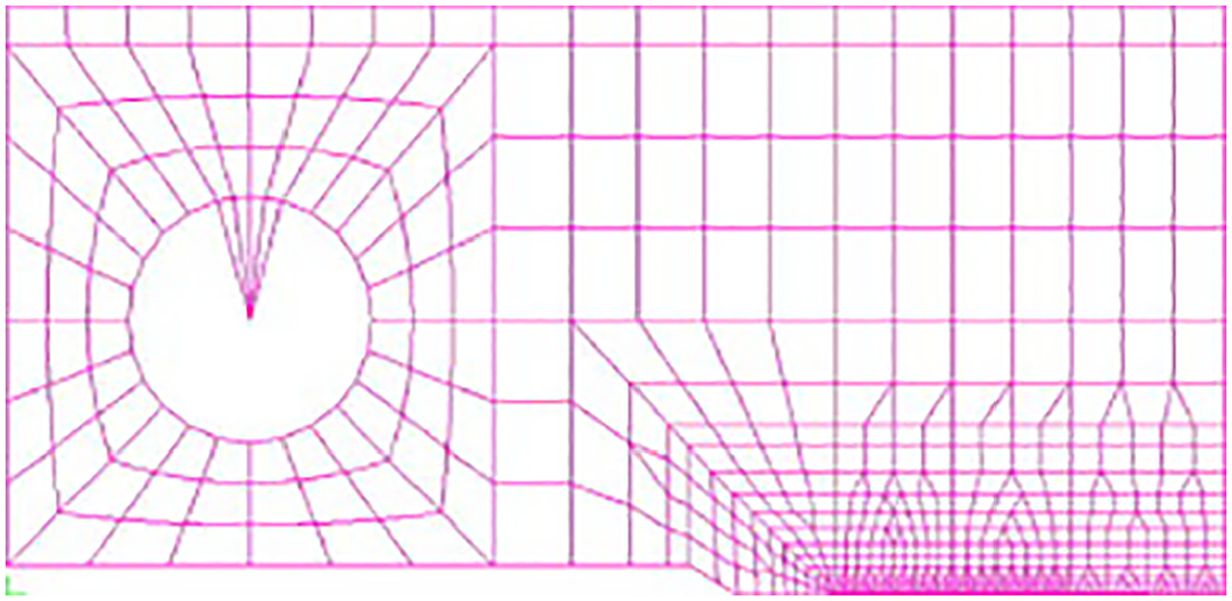
The discretized geometry of the specimen is depicted in Figure 1. To reduce computational complexity, the symmetry of the specimen about its vertical mid-plane is leveraged, allowing for a simulation of only the right half of the geometry. The triangular elements in the mesh represent a wedge idealized as an elastic continuum with equivalent isotropic elastic properties matching those of the 16 MND 5 steel. The center of the wedge corresponds to the centroid of the circular hole machined into the CT specimen. Boundary conditions are imposed by applying a controlled vertical displacement at the centroid of the wedge, simulating the load transfer mechanism and ensuring consistency with the experimental setup. This approach maintains the fidelity of the stress-strain response while optimizing computational resources.

In this study, a single 2D finite-element mesh is adopted, as a rigorous mesh sensitivity analysis was previously conducted in the numerical simulations of TA pre-cracked specimens, as reported by Enakoutsa et al. [7], Enakoutsa [12]. These earlier studies confirmed that the selected mesh density ensures sufficient spatial resolution for accurately capturing the localized stress and strain gradients near the crack tip, while maintaining computational efficiency. As a result, further mesh refinement or sensitivity analysis was deemed unnecessary for the present investigation, given the convergence and robustness demonstrated in prior work.

Figure 1.

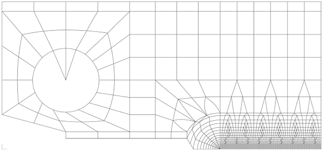
The figure presents the fine mesh configuration utilized in the computational analysis of the CTJ 25 pre-cracked specimen, which is critical for accurately capturing stress distribution and crack propagation. A refined mesh in finite element modeling enhances the simulation’s fidelity, particularly in areas with high stress gradients around the crack tip. This detailed mesh allows for precise calculations of the material’s mechanical response, facilitating a better understanding of how crack geometry and loading conditions affect fracture behavior. Ultimately, this careful meshing improves the accuracy of simulation results and aids in validating the modeling approach against experimental data.

In the experimental setup, the inclusion of lateral central triangular notches and the defined opening angle ensured that the region of crack propagation experienced near plane strain conditions, enabling a 2D numerical analysis. However, the assumption of ideal plane strain conditions is an approximation. To accurately correlate the simulation with the experimental results, the experimentally applied force must be normalized by an ”equivalent thickness” of the specimen, which accounts for deviations from the actual thickness in capturing the three-dimensional stress state. This correction has been rigorously investigated by Brosse [15], who determined an optimal equivalent thickness of 10.3 mm based on a detailed analysis of the stress distribution. This value is employed in the present study to enhance the fidelity of the simulation results. The material properties and constitutive parameters utilized in the model are listed in Table 2 in the Appendix 2. The hardening law is given as in the Figure 2. The elastic response is not explicitly represented, as its contribution is negligible and does not significantly influence the overall mechanical behavior of the material. 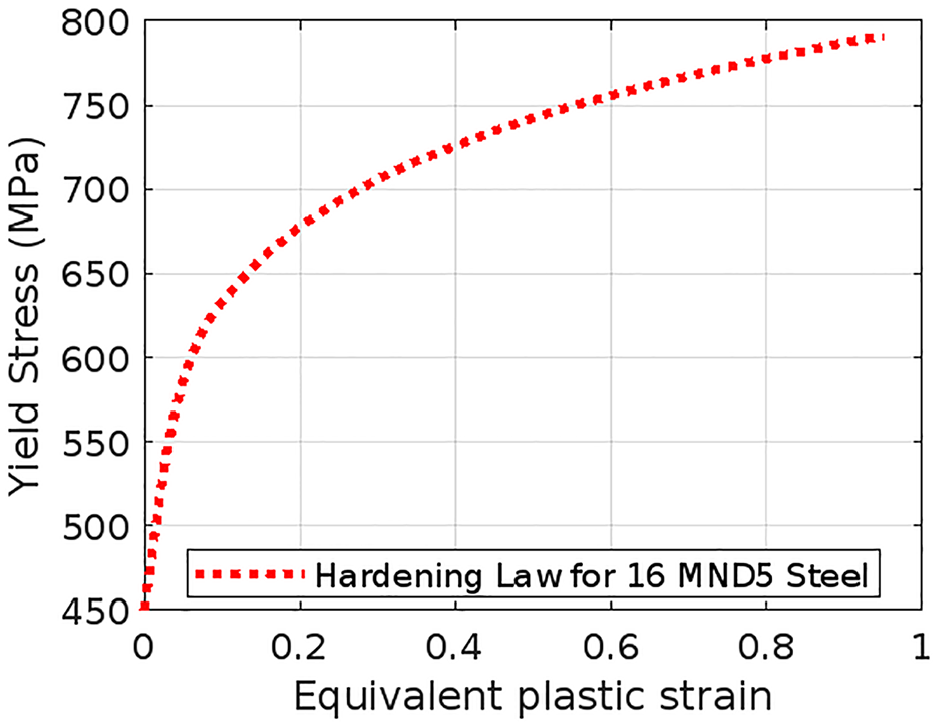The initial porosity value ( $f_{0}$ ) for this steel is determined based on the study by Murdy and Rousselier [16], which considers both the chemical composition and the inclusion state of the material. Specifically, $f_{0}$ is derived from the sulfur and manganese content, along with the average size of inclusions. Based on these factors, the initial porosity is determined to be 0.00016.

Figure 2.

Hardening Law of the 16 MND 5 Stainless Steel used in the Simulations, Brosse [15]. This figure illustrates the relationship between the plastic strain and the corresponding stress for the 16 MND 5 stainless steel. The data, derived from experimental measurements, highlights the material’s strain-hardening behavior, which is critical for accurately simulating deformation and fracture processes. The curve serves as the basis for calibrating the numerical model used in the study.

Figure 3 illustrates the experimental load–displacement curve (depicted by red points) in conjunction with the numerical results obtained via both kinematic and isotropic hardening formulations. The simulations reveal that the inclusion of kinematic hardening (results not presented here) yields negligible deviations from the isotropic hardening results, attributed to the uniaxial tension loading conditions employed in the numerical analysis. In addition, the initial iteration of the nonlocal damage model demonstrates excessive smoothing of the porosity distribution in the ligament region ahead of the crack tip, culminating in a significant and abrupt decrease in the load-displacement response (green curve). This anomaly can be rectified by implementing the natural logarithm in the porosity evolution equation, as depicted in Figure 3. However, the disparity between the numerical predictions derived from the modified nonlocal Gurson model (incorporating isotropic hardening) and the actual experimental data is markedly pronounced, necessitating urgent intervention. 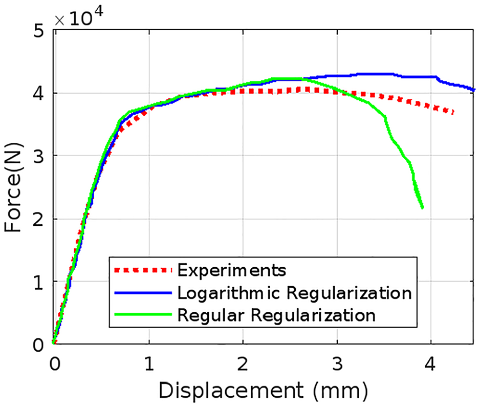This discrepancy can be effectively minimized through meticulous calibration of the parameters $f_{c}$ , representing the critical porosity threshold at the onset of coalescence, and the cavity growth acceleration factor δ, thus ensuring a robust alignment between theoretical predictions and experimental observations.

Figure 3.

A comprehensive comparison between the experimental and computed load–displacement curves for the CT specimen made of 16 MND 5 steel is presented for the cases of regular and logarithmic nonlocal regularizations. The experimental load–displacement data, derived from carefully conducted mechanical tests, provide crucial insights into the material’s behavior under applied loading conditions, including its resistance to crack initiation and propagation. These experimental results serve as a benchmark for evaluating the accuracy of the computational model used to simulate the material’s performance. The computed curves, generated through numerical simulations, are compared to the experimental data to assess the model’s predictive capability. This comparison not only highlights the model’s ability to replicate the observed load-bearing response but also helps identify any discrepancies, which may point to limitations in the current model or areas where additional refinement or parameter adjustments are necessary. By juxtaposing the experimental and computed results, this analysis provides a deeper understanding of the material’s mechanical behavior and offers a pathway for improving simulation techniques, ultimately enhancing the accuracy of future predictions for 16 MND 5 steel in various engineering applications.

4.8.2. Application 2: simulation of a 2D compact tension (CT12) specimen

As a second demonstration, we present a 2D simulation of Marie’s [17] fracture test on a CT12 specimen composed of SS 316L stainless steel, where CT 12 designates a specimen with a thickness of 12 mm. Figure 4 illustrates the discretized geometry, utilizing symmetry along the vertical mid-plane of the specimen to simplify modeling to only the right half, optimizing computational efficiency without compromising accuracy. The specimen dimensions are 25 mm in both width and height, with a 12 mm thickness.

The specimen features a carefully designed notch, 2 mm wide and extending to a depth of 85 mm from the top surface. This notch has a unique profile: it is rectangular near the surface but transitions into a triangular form with a sharp 60° opening angle at the root, simulating high-stress concentration areas. From the base of this notch, a 1.34 mm fatigue pre-crack propagates, further enhancing the focus on fracture mechanics under controlled initiation conditions.

Figure 4.

Discretized geometry of the CT12 specimen used in the 2D fracture test simulation. The model leverages symmetry along the vertical mid-plane to reduce computational complexity by simulating only the right half of the specimen. Key features include the rectangular-to-triangular notch profile with a 60° opening angle at the root, designed to create a controlled stress concentration. This setup allows for a detailed study of crack initiation and propagation under simulated fracture conditions in SS 316L stainless steel.

Figure 5.

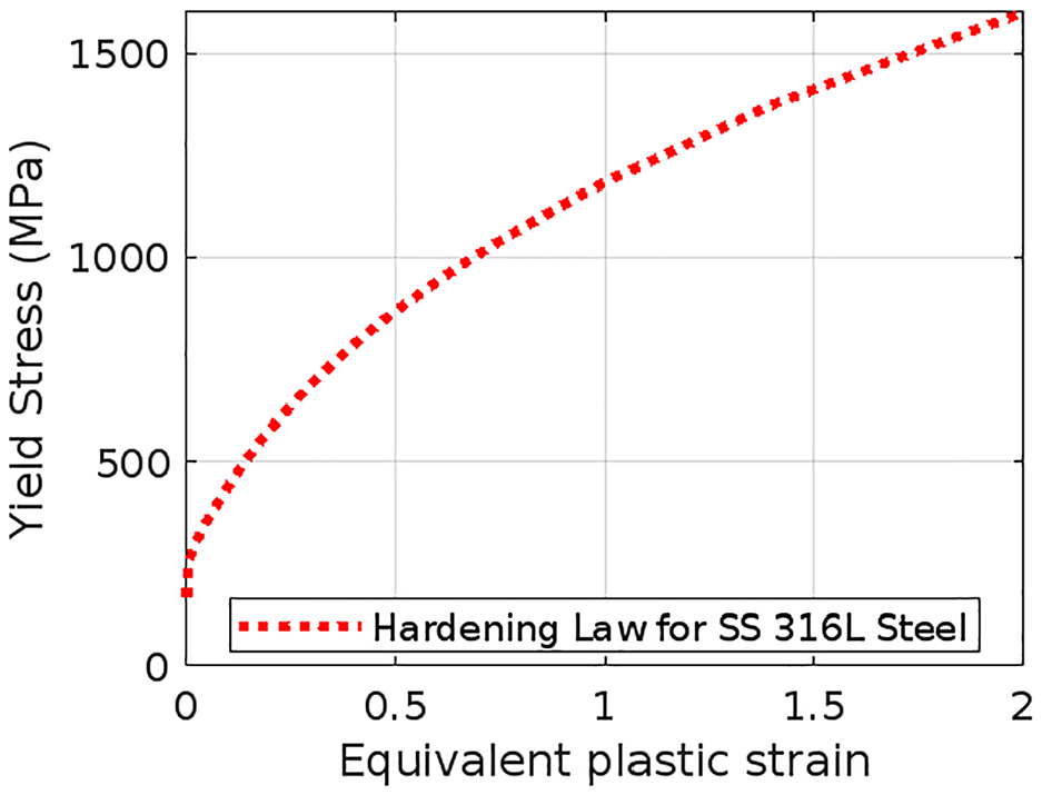
Hardening Law of the SS 315 L Stainless Steel used in the Simulations, Marie [17]. This figure depicts the stress-strain relationship for SS 315 L steel, highlighting its strain-hardening characteristics. The experimental data provides the foundation for modeling the material’s mechanical response under plastic deformation, ensuring accurate simulations of its behavior in structural applications.

Here also, a single 2D mesh is used since the issue of mesh sensitivity has already been considered quite comprehensively, in the works of Enakoutsa [12] and Enakoutsa et al. [7] in the numerical simulations of TA specimens.

In this experiment, lateral central triangular notches with a depth of $1.2 mm$ and an opening angle of approximately $45^{°}$ were introduced to establish plane strain conditions within the crack propagation zone, enabling accurate two-dimensional (2D) simulation. Given that the plane strain assumption introduces a minor approximation, a correction is required when comparing simulation results with experimental data. Specifically, the experimentally applied force must be scaled by an ”equivalent thickness” $t_{eq}$ to account for the actual specimen thickness discrepancy. Following the detailed analysis by Brosse [15], an equivalent thickness value of $t_{eq} = 10.3 mm$ is adopted here as the optimal adjustment factor. The material parameters are detailed in Appendix 3. The hardening law is given as in the Figure 5.

Figure 6.

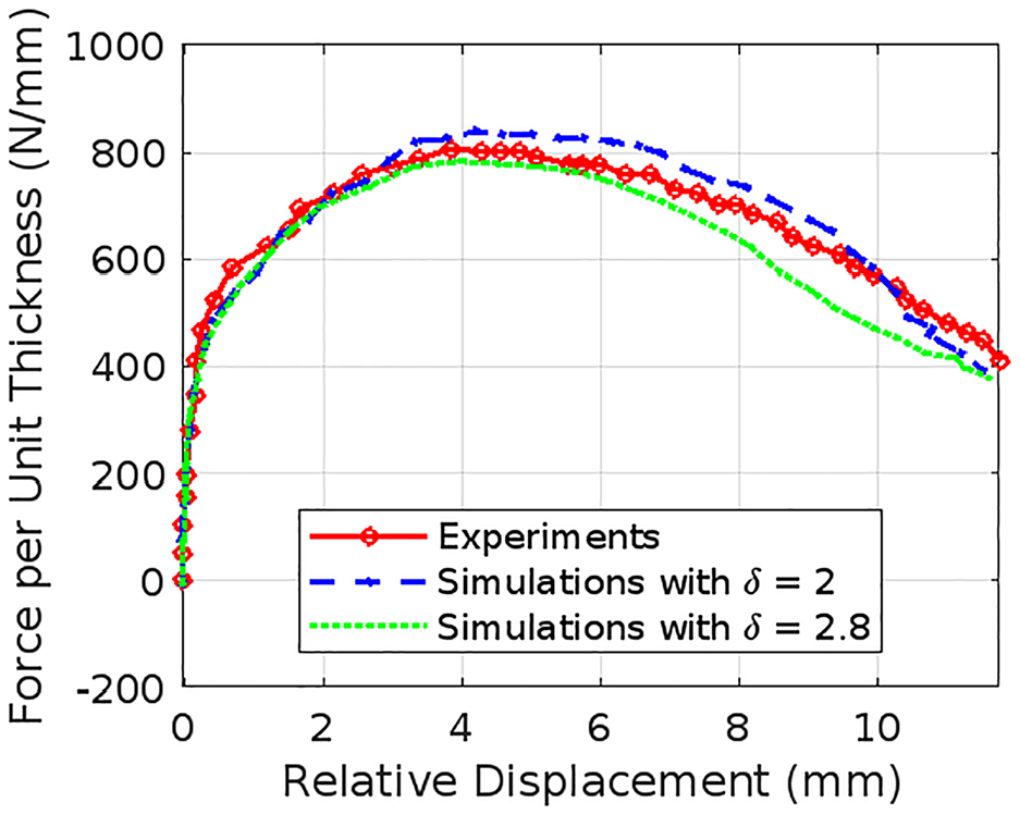
A detailed comparison of the experimental and computed load-displacement curves for the CT (Compact Tension) specimen of SS 316L stainless steel is presented. The experimental curves, obtained from physical tests, serve as a benchmark for validating the accuracy and predictive capabilities of the computational model. These curves illustrate the material’s response to loading and provide key insights into its fracture behavior under various conditions. The computed curves, derived from the nonlocal GLD model, are compared to the experimental data to assess the model’s ability to replicate the observed material response. This comparison not only highlights the model’s strengths but also reveals any discrepancies, which may point to areas where further refinement or adjustments are needed in the modeling approach. By juxtaposing the experimental and computational results, this analysis enables a deeper understanding of the material’s mechanical behavior and the effectiveness of the simulation techniques employed.

Figure 6 shows the experimental load-displacement curve (in red color) together with two numerical ones:

The blue curve shown in the figure has been obtained using the nonlocal GLD model, which incorporates the phenomenon of coalescence. The damage model parameters for coalescence were set to $f_{c} = 0.05$ and $δ = 2$ for a length scale of $400 μ m$ . The nearly agreement between the model’s prediction and the experimental data underscores the model’s ability to accurately reproduce experimental observations. This result is achieved by employing relatively high values of $f_{c}$ , which are consistent with the theoretical estimates obtained from micromechanical simulations of representative porous cells. These simulations provide valuable insights into the material behavior at the microscale, confirming that the chosen values of $f_{c}$ align with those predicted for porous materials in the context of coalescence and nonlocal effects.

The green curve has been generated using the same nonlocal GLD model, but with a significantly higher value of the coalescence accelerator parameter. This increased value leads to a pronounced discrepancy between the model prediction and the experimental data. The large deviation highlights the critical importance of accurately accounting for the coalescence mechanism in the model. Without properly capturing the influence of coalescence, the model fails to replicate the experimental results, emphasizing the necessity of fine-tuning the coalescence parameter to achieve a satisfactory fit. This observation underscores the sensitivity of the model to the choice of coalescence parameters and reinforces the need for a careful balance between the model’s theoretical foundations and experimental validation to ensure accurate predictions.

5. Conclusion

This paper has presented a comprehensive study of GSMs and their applications in metal plasticity and nonlocal damage models, addressing both theoretical and practical challenges. The GSM framework was shown to provide a robust and thermodynamically consistent foundation for modeling small strain von Mises plasticity and advanced ductile fracture mechanisms, such as those described by the GLD model. Numerical simulations of compact tension (CT) specimen fracture tests for two different steels highlighted the predictive accuracy and practical utility of the GLD framework, particularly in capturing the effects of cavity shape and porosity under realistic loading conditions.

For nonlocal damage models, two key theoretical results were established: the exponential attenuation of high-frequency components and the approximation of nonlocal formulations as diffusion-like equations. These findings underscore the regularizing nature of Gaussian kernels while highlighting the limitations of excessive smoothing, which can lead to unrealistic damage distributions. To address this, a modified evolution equation incorporating logarithmic terms was proposed, ensuring stability and spatial consistency while preserving the physical fidelity of the model. Furthermore, the sensitivity analysis of the length scale parameter l offered valuable insights into balancing regularization and physical accuracy, providing practical guidelines for the design and implementation of nonlocal formulations.

In conclusion, this work bridges critical gaps in the understanding and application of GSM and nonlocal damage models, offering both theoretical insights and practical tools for advancing the modeling of complex material behaviors. Future research should explore the extension of these findings to more diverse materials, loading conditions, and advanced numerical methods to further enhance their applicability and robustness.

Footnotes

Appendix 1

Appendix 2

Appendix 3

Appendix 4 Funding

The author(s) received no financial support for the research, authorship, and/or publication of this article.

ORCID iD

Koffi Enakoutsa

Notes

References

Halphen

Nguyen

. Sur les matériaux standards généralisés. J Mécanique 1975; 14: 39–63.

Ziegler

Wehrli

. The derivation of constitutive relations from the free energy and dissipation functions. Adv Appl Mech 1987; 25: 183–237.

Hackl

. Generalized standard media and variational principles in classical and finite strain elasto-plasticity. J Mech Phys Solids 1997; 45(5): 667–688.

Lee

. Elastic-plastic deformation at finite strain. J Appl Mech 1969; 36: 1–6.

Fremond

. Non-smooth thermomechanics. Berlin: Springer-Verlag, 2002.

Maugin

. The thermomechanics of plasticity and fracture. Cambridge: Cambridge University Press, 1992.

Enakoutsa

Leblond

Perrin

. Numerical implementation and assessment of a phenomenological nonlocal model of ductile rupture. Comput Meth Appl Mech Engng 2007; 196: 1946–1957.

Nguyen

. On the elastic plastic initial-boundary value problem and its numerical integration. Int J Numer Meth Engng 1977; 11: 817–832.

Gologanu

Leblond

Perrin

, et al. Recent extensions of Gurson’s model for porous ductile metals. In: Suquet

(ed.) Continuum micromechanics, CISM courses and lectures, vol. 377. Cham: Springer, 1997, pp. 61–130.

10.

Tvergaard

. Influence of voids on shear band instabilities under plane strain conditions. Int J Fracture 1981; 17: 389–407.

11.

Gurson

. Continuum theory of ductile rupture by void nucleation and growth: part I - yield criteria and flow rules for porous ductile media. ASME J Engng Materials Technol 1977; 99: 2–15.

12.

Enakoutsa

. Modèle non-locaux en rupture ductile des métaux. PhD Thesis, Université Pierre et Marie Curie (Paris VI), Paris, 2007. (In French)

13.

Son

. On the elastic plastic initial-boundary value problem and its numerical integration. Int J Num Meth Eng 1977; 11: 817–832.

14.

Devaux

Mottet

. Etude Numérique de la Rupture Ductile de l’Acier de Cuve 16MND5: Simulation des Eprouvettes Fissurées de Type TA et CTJ. Technical Report LTSW.92/2036, ESI, Lyon, 1992.

15.

Brosse

. Modélisation de déchirure ductile dans un tuyau inox – Calage des paramètres de Wilkins. Technical Report F/LE/09/042/D/BPE, ESI France, Lyon, 2009. (In French)

16.

Rousselier

Mudry

. Etude de la rupture ductile de l’acier faiblement allié en Mn-Ni-Mo pour cuves de réacteurs à eau ordinaire sous pression, approvisionné sous la forme d’une débouchure de tubulure. Résultats du programme expérimental. Technical Report HT/PV D529 MAT/T43, EdF Centre des Renardières, Moret-Loing-et-Orvanne, 1983. (In French)

17.

Marie

. Méthodes de prédiction de grandes déchirures: données expérimentales nécessaires aux modélisations. Technical Report SEMT/LISN/RT/00-020, CEA, 2000. (In French)