Bayesian operator learning for nonlocal damage mechanics and internal length scale identification

Abstract

We develop a Bayesian operator-learning framework for nonlocal damage mechanics aimed at calibrating uncertain internal length scales and quantifying predictive uncertainty from limited observations. The deterministic forward model is based on an AT2-type gradient damage regularization, which introduces a finite localization width and provides a mesh-objective continuum description of strain-softening behavior. The resulting boundary-value problem is interpreted as a parametric solution map from loading and material parameters to displacement and damage fields in Sobolev spaces. To accelerate the repeated forward evaluations required in Bayesian inversion, we introduce a learned surrogate approximation of this nonlinear operator. The present numerical implementation employs a computationally efficient convolutional surrogate with Monte Carlo-dropout uncertainty quantification, while the overall framework is formulated in an architecture-agnostic manner and can be extended to richer neural-operator constructions in future work. A principal contribution of the paper concerns parameter identifiability in the pre-critical regime. We show that when only global traction–displacement observations are available, the Fisher information associated with the internal length scale may become small. Consequently, the inverse problem can be practically nonidentifiable: materially distinct parameter values may generate nearly indistinguishable global responses, yielding diffuse or biased posterior distributions despite apparently accurate curve fits. Numerical experiments on a 1D benchmark validate this mechanism. The posterior distribution of the internal length scale is shown to remain weakly informative under monotone pre-critical loading, even though the global traction–displacement response is predicted accurately. In addition, field-level predictive uncertainty is observed to concentrate near mechanically active damage zones, highlighting spatial regions where additional measurements would be most informative. The proposed framework provides a mathematically consistent and computationally efficient route toward probabilistic calibration of nonlocal damage models. The most strongly validated conclusion of the present study is that accurate global response prediction does not necessarily imply reliable identification of internal length scales. Extensions to post-peak snap-back regimes, instability-enhanced identifiability, and multidimensional operator-learning architectures are left for future work.

Keywords

nonlocal damage mechanics operator learning uncertainty quantification internal length scale identification machine learning

1. Introduction

1.1. Nonlocal damage and variational fracture regularization

Strain localization and mesh-sensitive softening are endemic to local continuum damage and ductile degradation models: once the constitutive tangent loses ellipticity, the governing boundary-value problem may become ill-posed and numerical solutions collapse onto the discretization scale. Two broad and mathematically grounded regularization routes have emerged. The first is nonlocal/gradient damage, where internal length scales enter through integral-type averaging or higher-order gradients, thereby restoring well-posedness and selecting a finite localization width [1 –3]. The second is the variational approach to fracture initiated by Francfort–Marigo, where crack evolution is driven by global energy minimization under irreversibility [4]. In computational practice, the sharp crack functional is approximated by elliptic phase-field regularizations (Ambrosio–Tortorelli type), leading to robust algorithms and a clear interpretation of the length scale as the width of a diffused damage zone [5 –8]. These phase-field models (including the widely used AT2 formulation) have become a standard platform for predicting initiation, propagation, and complex crack topologies in brittle and quasi-brittle solids [9, 10].

At the same time, the contemporary continuum-mechanics literature has developed several alternative damage paradigms that go beyond the classical scalar gradient-damage setting. These include hemivariational formulations for strain-gradient elasto-plastic-damage solids with granular microstructure [11], intrinsic second-gradient and micro-morphology-informed models for pantographic and grain–grain interaction effects [12], as well as microdamage-informed biomechanical remodeling frameworks in which damage interacts with long-time structural adaptation in living tissues [13, 14]. Such contributions show that damage should not be viewed solely as a regularization device for localization but also as a multiscale internal variable whose interpretation depends on the underlying microstructure, morphology, and even biological remodeling mechanisms. This broader perspective is important for the present work: our focus is on an AT2-type gradient damage model, but the inverse and uncertainty-quantification issues we address are part of a larger class of continuum models in which internal length scales, microstructural parameters, and degradation descriptors must be inferred from incomplete observations.

1.2. Snap-back, post-peak response, and the need for path-following

Even with a sound regularization, quasi-static failure of notched or weakly heterogeneous specimens often exhibits limit points and snap-back in global response, i.e., a decreasing load with increasing displacement under certain control protocols. Capturing such post-peak behavior requires continuation strategies beyond basic load/displacement stepping, notably arc-length methods and their variants [15, 16]. For phase-field/gradient damage, this numerical issue is not cosmetic: the inferred fracture parameters (e.g., ℓ and $G_{c}$ ) can be structurally biased if the calibration data traverse an unstable branch, but the forward solver cannot reproduce it. These observations motivate future extensions of Bayesian calibration to genuine post-peak regimes. In the present paper, however, the reported computations are intentionally restricted to stable pre-critical loading paths to isolate identifiability mechanisms in the simplest controlled setting.

1.3. Inverse problems: calibration, uncertainty, and identifiability

Inferring internal length scales and toughness-like parameters from experiments is a prototypical ill-posed inverse problem: multiple parameter combinations can fit limited observations, and model discrepancy (geometry, boundary conditions, noise, and constitutive simplifications) can dominate [17 –19]. A Bayesian formulation promotes unknowns to random variables and yields a posterior distribution that quantifies uncertainty and correlations, enabling principled prediction and risk assessment [17, 20]. However, Bayesian inversion is only meaningful if the forward map is sufficiently informative. This raises a central identifiability question for nonlocal damage: Which data (global reaction curves, local fields, multi-load paths) actually identify ℓ and $G_{c}$ , and to what extent are they confounded? In gradient/phase-field settings, both ℓ and $G_{c}$ influence the dissipated energy and the localization width, suggesting that global energetics alone can be insufficient, while field measurements (e.g., full-field displacement/strain or damage proxies) can break degeneracies [2,3, 10]. Related identification questions also arise in structurally different contexts, e.g., in the use of genetic algorithms for the identification of collapse mechanisms in nonlinear masonry analysis [21]. Although the mechanical setting there differs from gradient damage, the underlying methodological lesson is similar: inverse identification in nonlinear mechanics is highly sensitive to the richness of the observable data and to the expressive power of the computational model used in the calibration loop. The present study focuses precisely on this issue by examining how informative global reaction data are for identifying the internal length scale in a pre-critical regime.

1.4. Why neural operators for nonlocal damage?

High-fidelity phase-field/gradient damage solvers are computationally intensive when repeated across parameter samples, geometries, and loading histories as required by Bayesian inference. This bottleneck is amplified in two-dimensional (2D)/three-dimensional (3D) and in the presence of snap-back, where continuation and inner alternate minimization loops are needed. Recent progress in operator learning addresses precisely this setting: rather than learning a single solution, neural operators learn mappings between function spaces, enabling fast emulation of partial differential equation (PDE) solution operators across families of inputs [22 –24]. Among these, the Fourier Neural Operator (FNO) has demonstrated strong performance for parametric PDEs with mesh-invariant generalization [22]. For nonlocal damage, the learned operator naturally accommodates (1) spatially varying material fields (e.g., $G_{c} (x)$ , weak spots), (2) boundary/loading controls, and (3) outputs as full fields (damage and displacement), which are exactly the objects needed to improve identifiability beyond scalar reaction data. More broadly, the appeal of operator learning in continuum damage mechanics lies in its potential to interface naturally with generalized continua in which the state variables may include gradients, microstructural descriptors, or remodeling fields, as illustrated by recent higher-gradient and microdamage-informed formulations [11 –14]. In the present benchmark study, the surrogate methodology is used in a reduced one-dimensional (1D) setting, while higher-dimensional neural-operator realizations remain a natural extension.

1.5. Bayesian neural operators and posterior field distributions

Beyond point predictions, uncertainty quantification (UQ) in learned surrogates is essential in inverse problems: surrogate error otherwise leaks into the posterior and yields overconfident inferences. Bayesian deep learning provides several scalable approximations, including Monte Carlo (MC)-dropout, variational Bayesian neural networks, and deep ensembles [25 –27]. In the operator-learning context, these tools enable posterior predictive distributions over fields, producing spatial maps of uncertainty that can concentrate near localization bands and crack paths—precisely where modeling and discretization errors are largest. This motivates a Bayesian operator-learning pipeline: (a) a physically consistent nonlocal damage solver generates training data and synthetic observations; (b) a surrogate model learns the parameter-to-field and load-to-field maps; (c) Bayesian inference is performed for $(ℓ, G_{c})$ using reaction and, when available, field data while propagating surrogate uncertainty. In the present paper, the numerical emphasis is on UQ for a 1D benchmark rather than on a full multidimensional deployment.

1.6. Scope and contribution of this work

This paper develops a Bayesian operator-learning framework for nonlocal damage with three interlocked goals: (1) physics fidelity: we adopt a variational AT2-type gradient damage formulation with irreversibility as the deterministic forward model; (2) Bayesian calibration: we infer $(ℓ, G_{c})$ from reaction data, quantify posterior correlations, and analyze identifiability mechanisms, with particular emphasis on weak informativeness of global data in pre-critical regimes; (3) operator-level surrogates with uncertainty: we employ learned surrogates to accelerate Bayesian inversion and report posterior field distributions, highlighting spatially localized epistemic uncertainty. By coupling variational nonlocal mechanics with Bayesian operator learning, the framework targets both computational scalability and statistically defensible inference for internal length scales in damage and fracture, while remaining conceptually connected to the broader family of generalized damage theories now emerging in continuum mechanics. The present numerical results are intentionally narrow in scope and serve as a rigorous baseline for future studies involving snap-back branches, multidimensional localization, and richer operator-learning architectures.

The present manuscript intentionally focuses on a controlled 1D benchmark so as to isolate identifiability mechanisms under weakly informative observations. Accordingly, numerical conclusions should be interpreted at this benchmark level, while broader multidimensional neural-operator developments remain future work.

1.7. Organization of the paper

The remainder of the paper is organized as follows. Section 2 introduces the deterministic nonlocal damage model and its variational formulation. We present the kinematical assumptions, the functional setting in Sobolev spaces, and the free-energy functional governing the coupled displacement–damage problem. Section 3 derives the governing Euler–Lagrange equations and discusses the associated equilibrium and nonlocal damage evolution equations together with the irreversibility constraint. Section 4 analyzes the variational structure of the problem and discusses existence, stability, and the role of the internal length scale in restoring well-posedness in strain-softening regimes. Section 5 describes the deterministic numerical strategy used to compute the equilibrium path, including the alternating minimization scheme and continuation methodology. Section 6 formulates the Bayesian inverse problem for identifying model parameters, with emphasis on the internal length scale and its identifiability from reaction data. Section 7 introduces the operator-learning formulation used to approximate the parametric solution operator of the damage model. Section 8 presents the Bayesian training framework for the surrogate model, including variational inference, posterior prediction, and the physics-consistency regularization used in the learning procedure. Section 9 reports the numerical results and discusses deterministic responses, Bayesian parameter inference, and field-level posterior uncertainty. Finally, Section 10 summarizes the main findings and outlines perspectives for future research.

Notation

To improve readability, we adopt the following conventions throughout the manuscript:

$D (x)$ denotes the continuum damage field in the analytical formulation.

d denotes its discrete numerical representation on a computational grid.

$G$ denotes a generic deterministic forward operator.

$G_{0}$ denotes the unknown ground-truth operator generating synthetic observations.

θ denotes physical model parameters (primarily the internal length scale ℓ).

ϕ denotes trainable surrogate-model parameters.

2. Deterministic nonlocal damage model

2.1. Modeling scope and interpretation

For clarity, we distinguish two closely related formulations used throughout this paper.

First, Sections 2–4 introduce a stationary variational gradient-damage model that serves as the analytical reference formulation. Its purpose is to define the regularized free energy, establish structural properties of the deterministic forward problem, and provide the mathematical setting for operator-learning approximation and Bayesian inversion.

Second, the numerical experiments reported later in Section 9 employ the standard incremental irreversible AT2 phase-field formulation with loading steps, history-field updates, and the constraint of nondecreasing damage. That computational model introduces path dependence and corresponds to the practical evolution setting commonly used in phase-field fracture simulations.

The two formulations share the same energetic ingredients—elastic degradation, fracture toughness, and internal length-scale regularization—but they are mathematically distinct. Unless explicitly stated otherwise, all existence, stability, and variational results in Sections 2–4 concern the stationary reference model, whereas the numerical results concern the irreversible incremental solver described in the computational framework.

2.2. Kinematics and functional setting

We begin by introducing the kinematical assumptions and the functional framework underlying the stationary nonlocal damage model. The formulation is restricted to the regime of infinitesimal deformations and is posed within a Sobolev space setting suitable for variational analysis.

Let $Ω \subset ℝ^{d}$ , with $d = 2, 3$ , denote an open bounded Lipschitz domain representing the reference configuration of the body. Its boundary $\partial Ω$ is decomposed into two disjoint measurable parts,

\partial Ω = Γ_{D} \cup Γ_{N}, Γ_{D} \cap Γ_{N} = \emptyset,

where $Γ_{D}$ and $Γ_{N}$ correspond to the Dirichlet and Neumann boundary portions, respectively.

The primary kinematic unknown is the displacement field

u : Ω \to ℝ^{d},

assumed sufficiently regular to admit square-integrable weak derivatives. Under the hypothesis of small strains, the symmetric infinitesimal strain tensor is defined by

\begin{matrix} ε (u) = \frac{1}{2} (\nabla u + {(\nabla u)}^{⊤}) \in ℝ_{sym}^{d \times d}, \end{matrix}

(1)

where $\nabla u$ denotes the displacement gradient and ${(⋅)}^{⊤}$ its transpose. The tensor $ε (u)$ represents the linearized measure of deformation and belongs to $L^{2} (Ω; ℝ_{sym}^{d \times d})$ whenever $u \in H^{1} (Ω; ℝ^{d})$ .

Material degradation is described by a scalar damage field

D : Ω \to [0, 1],

which modulates the elastic response through a stiffness reduction mechanism. The bounds $0 \leq D \leq 1$ are interpreted physically as the transition from undamaged material ( $D = 0$ ) to complete loss of stiffness ( $D = 1$ ). In the present stationary formulation, D is treated as an equilibrium internal variable. Irreversibility constraints are introduced later only in the incremental numerical model.

The natural functional setting for the coupled displacement–damage problem is the product Sobolev space

H^{1} (Ω; ℝ^{d}) \times H^{1} (Ω),

which guarantees square-integrable fields and gradients. Incorporating the essential boundary condition $u = u_{D}$ on $Γ_{D}$ , with prescribed displacement $u_{D} \in H^{1 ∕ 2} (Γ_{D}; ℝ^{d})$ , we define the admissible space

\begin{matrix} V = {(u, D) \in H^{1} (Ω; ℝ^{d}) \times H^{1} (Ω) : u = u_{D} on Γ_{D}} . \end{matrix}

(2)

This Hilbert-space structure provides the appropriate framework for the stationary variational problem developed below.

2.3. Free energy functional

We formulate the stationary nonlocal damage model within a variational framework. The constitutive structure is defined by a Helmholtz-type gradient regularization that introduces an intrinsic material length scale and restores ellipticity in softening regimes.

Let $Ω \subset ℝ^{d}$ , $d = 2, 3$ , be a bounded Lipschitz domain. The primary variables are the displacement field $u : Ω \to ℝ^{d}$ and the scalar damage field $D : Ω \to [0, 1]$ . Under the small-strain assumption, the infinitesimal strain tensor is

\begin{matrix} ε (u) = \frac{1}{2} (\nabla u + \nabla u^{⊤}) . \end{matrix}

(3)

The total free energy functional is defined as

\begin{matrix} E (u, D) = \int_{Ω} ψ (ε (u), D, \nabla D) d Ω, \end{matrix}

(4)

where the energy density is given by

\begin{matrix} ψ = {(1 - D)}^{m} \frac{1}{2} ε (u) : C : ε (u) + \frac{G_{c}}{2 ℓ} D^{2} + \frac{G_{c} ℓ}{2} | \nabla D |^{2} . \end{matrix}

(5)

The fourth-order elasticity tensor C satisfies the classical minor and major symmetries

\begin{matrix} C_{ijkl} = C_{jikl} = C_{ijlk} = C_{klij}, \end{matrix}

(6)

together with the uniform ellipticity condition

\begin{matrix} ε : C : ε \geq c_{0} | ε |^{2}, c_{0} > 0, \end{matrix}

(7)

for all symmetric second-order tensors $ε \in ℝ_{sym}^{d \times d}$ . The exponent $m \geq 1$ governs the degradation of stiffness, $G_{c} > 0$ denotes the fracture toughness, and $ℓ > 0$ is the internal length scale that controls the width of the regularized damage zone.

We emphasize that (4) defines the stationary reference problem used for analysis. In the irreversible incremental formulation employed numerically, the same energetic ingredients are minimized sequentially under history dependence and monotonicity constraints on damage.

2.3.1. Coercivity and weak lower semicontinuity

Under the nondegeneracy condition stated below, the gradient contribution together with the bounded degradation law yields coercivity on the admissible class.

Proposition 2.1 (Conditional coercivity and existence). Assume that C satisfies (7), $m \geq 1$ , $G_{c} > 0$ , and $ℓ > 0$ . Assume moreover that the admissible damage fields satisfy

0 \leq D \leq d_{\max} < 1 a.e. in Ω,

and that $Γ_{D}$ has positive surface measure. Then, the functional $E$ is coercive on the admissible class

A = {(u, D) \in H^{1} (Ω; ℝ^{d}) \times H^{1} (Ω) : u = u_{D} on Γ_{D}, 0 \leq D \leq d_{\max} < 1} .

Moreover, $E$ is weakly lower semicontinuous on $A$ . Consequently, $E$ admits at least one minimizer in $A$ .

If the constraint $D \leq d_{\max} < 1$ is not imposed, the same conclusion holds provided the degradation law is regularized as

g (D) = {(1 - D)}^{m} + κ, κ > 0 .

Proof 1. Let $(u, D) \in A$ . Since

0 \leq D \leq d_{\max} < 1,

we have the uniform lower bound

{(1 - D)}^{m} \geq {(1 - d_{\max})}^{m} = : g_{\min} > 0 .

Using the ellipticity of C, namely

ε : C : ε \geq c_{0} | ε |^{2},

we obtain

{(1 - D)}^{m} ε (u) : C : ε (u) \geq c_{0} g_{\min} | ε (u) |^{2} .

Therefore,

\int_{Ω} {(1 - D)}^{m} \frac{1}{2} ε (u) : C : ε (u) d Ω \geq \frac{c_{0} g_{\min}}{2} ∥ ε (u) ∥_{L^{2} (Ω)}^{2} .

Since $Γ_{D}$ has positive measure, Korn’s inequality on the Dirichlet admissible space gives

∥ u ∥_{H^{1} (Ω)} \leq C_{K} (∥ ε (u) ∥_{L^{2} (Ω)} + ∥ u_{D} ∥_{H^{1 ∕ 2} (Γ_{D})}) .

Thus, the elastic term controls the $H^{1}$ -norm of u up to a constant depending only on the prescribed boundary data.

For the damage variable, the local and gradient terms satisfy

\int_{Ω} (\frac{G_{c}}{2 ℓ} D^{2} + \frac{G_{c} ℓ}{2} | \nabla D |^{2}) d Ω \geq c_{D} ∥ D ∥_{H^{1} (Ω)}^{2},

with

c_{D} = \frac{1}{2} \min {\frac{G_{c}}{ℓ}, G_{c} ℓ} > 0 .

Combining the displacement and damage estimates yields

E (u, D) \geq C_{1} ∥ u ∥_{H^{1} (Ω)}^{2} + C_{2} ∥ D ∥_{H^{1} (Ω)}^{2} - C_{3},

for constants $C_{1}, C_{2} > 0$ and $C_{3} \geq 0$ . Hence, $E$ is coercive on $A$ .

We now prove weak lower semicontinuity. Let

(u_{n}, D_{n}) ⇀ (u, D) weakly in H^{1} (Ω; ℝ^{d}) \times H^{1} (Ω),

with $(u_{n}, D_{n}) \in A$ . Since $A$ is weakly closed, the limit also satisfies

u = u_{D} on Γ_{D}, 0 \leq D \leq d_{\max} < 1 .

By compactness of the embedding $H^{1} (Ω) ↪ L^{2} (Ω)$ , up to a subsequence,

D_{n} \to D strongly in L^{2} (Ω) and a.e. in Ω .

Because $0 \leq D_{n} \leq d_{\max}$ , the functions

g (D_{n}) = {(1 - D_{n})}^{m}

are uniformly bounded above and below, and

g (D_{n}) \to g (D) strongly in L^{q} (Ω)

for every finite $q \geq 1$ .

Set

A_{n} (x) = g {(D_{n} (x))}^{1 ∕ 2} C^{1 ∕ 2} ε (u_{n}) (x) .

Since $ε (u_{n}) ⇀ ε (u)$ in $L^{2}$ and $g {(D_{n})}^{1 ∕ 2} \to g {(D)}^{1 ∕ 2}$ strongly in $L^{q}$ for every finite q, we have

A_{n} ⇀ g {(D)}^{1 ∕ 2} C^{1 ∕ 2} ε (u) weakly in L^{2} (Ω) .

By weak lower semicontinuity of the $L^{2}$ norm,

\int_{Ω} g (D) ε (u) : C : ε (u) d Ω \leq \underset{n \to \infty}{\lim \inf} \int_{Ω} g (D_{n}) ε (u_{n}) : C : ε (u_{n}) d Ω .

The damage terms are convex quadratic functionals of D and $\nabla D$ ; therefore,

\int_{Ω} (\frac{G_{c}}{2 ℓ} D^{2} + \frac{G_{c} ℓ}{2} | \nabla D |^{2}) d Ω \leq \underset{n \to \infty}{\lim \inf} \int_{Ω} (\frac{G_{c}}{2 ℓ} D_{n}^{2} + \frac{G_{c} ℓ}{2} | \nabla D_{n} |^{2}) d Ω .

Combining the two lower semicontinuity estimates gives

E (u, D) \leq \underset{n \to \infty}{\lim \inf} E (u_{n}, D_{n}) .

Thus, $E$ is weakly lower semicontinuous on $A$ .

Finally, let ${(u_{n}, D_{n})}$ be a minimizing sequence in $A$ . Coercivity gives boundedness in $H^{1} (Ω; ℝ^{d}) \times H^{1} (Ω)$ . By reflexivity, there is a weakly convergent subsequence. Since $A$ is weakly closed, the limit belongs to $A$ . Weak lower semicontinuity then implies that the limit is a minimizer of $E$ .

If, instead, one uses the regularized degradation law $g (D) = {(1 - D)}^{m} + κ$ with $κ > 0$ , the same proof applies with $g_{\min} = κ$ , without requiring the upper bound $D \leq d_{\max} < 1$ .

The internal length ℓ enters exclusively through the Helmholtz-type operator associated with the damage field. It controls the energetic penalty on gradients of D and therefore selects a finite localization width, thereby preventing pathological mesh-dependent collapse in the softening regime.

2.4. First variation and governing equations

We now derive the Euler–Lagrange equations associated with the nonlocal damage functional. The derivation clarifies the thermodynamic structure and establishes the coupled equilibrium–damage system in both weak and strong form.

2.4.1. Energy functional and admissible space

Let $Ω \subset ℝ^{d}$ ( $d = 2, 3$ ) be a bounded Lipschitz domain with boundary $\partial Ω = Γ_{D} \cup Γ_{N}$ , $Γ_{D} \cap Γ_{N} = \emptyset$ . The displacement field is $u : Ω \to ℝ^{d}$ and the scalar damage variable is $D : Ω \to [0, 1]$ .

The total free energy reads

\begin{matrix} E (u, D) = \int_{Ω} ψ (ε (u), D, \nabla D) d Ω - \int_{Ω} b \cdot u d Ω - \int_{Γ_{N}} t \cdot u d Γ, \end{matrix}

(8)

where the strain tensor is

ε (u) = \frac{1}{2} (\nabla u + \nabla u^{⊤}),

and the stored energy density is

\begin{matrix} ψ = {(1 - D)}^{m} \frac{1}{2} ε : C : ε + \frac{G_{c}}{2 ℓ} D^{2} + \frac{G_{c} ℓ}{2} | \nabla D |^{2} . \end{matrix}

(9)

The elasticity tensor C is assumed symmetric and uniformly elliptic, $G_{c} > 0$ , $ℓ > 0$ , and $m \geq 1$ .

Admissible variations $(δ u, δD)$ satisfy

δ u = 0 on Γ_{D}, δD \in H^{1} (Ω) .

2.4.2. First variation

Let $(u_{ε}, D_{ε}) = (u, D) + ε (δ u, δD)$ . Differentiating (8) with respect to ε at $ε = 0$ yields

δ E = {\frac{d}{dε} E (u_{ε}, D_{ε}) |}_{ε = 0} .

Using (9), we compute

\begin{matrix} \frac{∂ψ}{\partial ε} = {(1 - D)}^{m} C : ε, \frac{∂ψ}{∂D} = - m {(1 - D)}^{m - 1} \frac{1}{2} ε : C : ε + \frac{G_{c}}{ℓ} D, \\ \frac{∂ψ}{\partial \nabla D} = G_{c} ℓ \nabla D . \end{matrix}

Therefore,

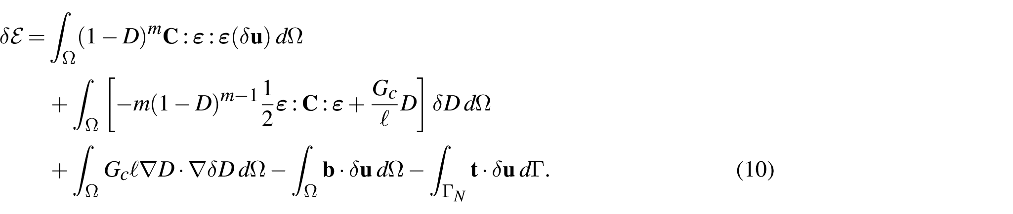
\begin{matrix} δ E & = \int_{Ω} {(1 - D)}^{m} C : ε : ε (δ u) d Ω \\ + \int_{Ω} [- m {(1 - D)}^{m - 1} \frac{1}{2} ε : C : ε + \frac{G_{c}}{ℓ} D] δD d Ω \\ + \int_{Ω} G_{c} ℓ \nabla D \cdot \nabla δD d Ω - \int_{Ω} b \cdot δ u d Ω - \int_{Γ_{N}} t \cdot δ u d Γ . \end{matrix}

(10)

2.4.3. Integration by parts and weak form

We define the Cauchy stress tensor

\begin{matrix} σ = \frac{∂ψ}{\partial ε} = {(1 - D)}^{m} C : ε . \end{matrix}

(11)

For the displacement variation, no further integration by parts is required, since

σ : ε (δ u) = σ : \nabla^{s} δ u .

For the damage gradient term, we integrate by parts:

\int_{Ω} G_{c} ℓ \nabla D \cdot \nabla δD d Ω = - \int_{Ω} G_{c} ℓ Δ D δD d Ω + \int_{\partial Ω} G_{c} ℓ (\nabla D \cdot n) δD d Γ .

Substituting into (10), we obtain

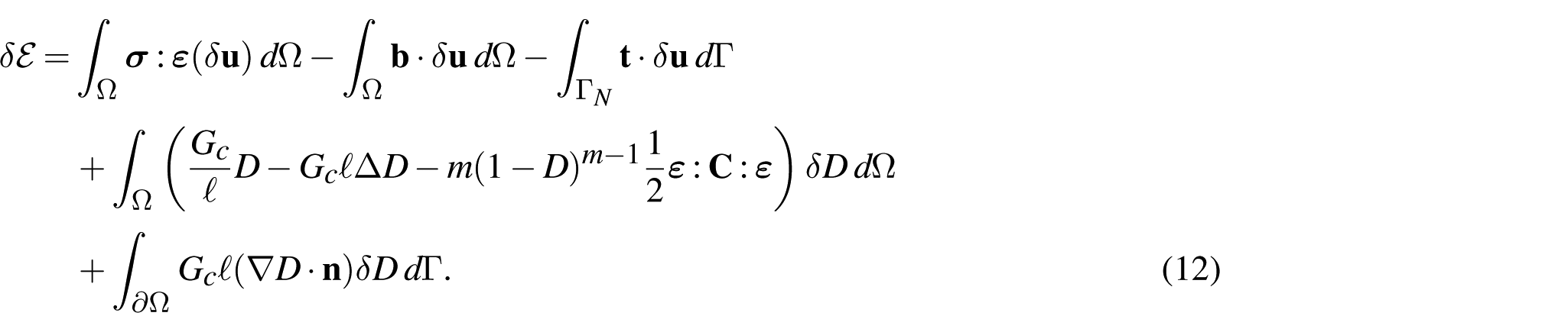
\begin{matrix} δ E & = \int_{Ω} σ : ε (δ u) d Ω - \int_{Ω} b \cdot δ u d Ω - \int_{Γ_{N}} t \cdot δ u d Γ \\ + \int_{Ω} (\frac{G_{c}}{ℓ} D - G_{c} ℓ Δ D - m {(1 - D)}^{m - 1} \frac{1}{2} ε : C : ε) δD d Ω \\ + \int_{\partial Ω} G_{c} ℓ (\nabla D \cdot n) δD d Γ . \end{matrix}

(12)

2.4.4. Stationarity condition

Equilibrium corresponds to $δ E = 0$ for all admissible variations.

Theorem 2.2 (First-order optimality and Euler–Lagrange system). Let

E (u, D) = \int_{Ω} [g (D) \frac{1}{2} ε (u) : C : ε (u) + \frac{G_{c}}{2 ℓ} D^{2} + \frac{G_{c} ℓ}{2} | \nabla D |^{2}] d Ω - \int_{Ω} b \cdot u d Ω - \int_{Γ_{N}} t \cdot u d Γ,

where

g (D) = {(1 - D)}^{m}, m \geq 1, G_{c} > 0, ℓ > 0,

and where C is symmetric and uniformly elliptic on symmetric tensors.

Let

(u, D) \in H^{1} (Ω; ℝ^{d}) \times H^{1} (Ω)

be a stationary point of $E$ with respect to admissible variations

δ u \in H_{Γ_{D}}^{1} (Ω; ℝ^{d}), δD \in H^{1} (Ω) .

Assume, for the purpose of deriving the equality form of the Euler–Lagrange equation, that the damage constraint is inactive, namely that variations $D + sδD$ remain admissible for all sufficiently small $| s |$ .

Then, $(u, D)$ satisfies the weak equilibrium equation

\begin{matrix} \int_{Ω} g (D) C : ε (u) : ε (δ u) d Ω = \int_{Ω} b \cdot δ u d Ω + \int_{Γ_{N}} t \cdot δ u d Γ \end{matrix}

(13)

for all $δ u \in H_{Γ_{D}}^{1} (Ω; ℝ^{d})$ , and the weak damage equation

\begin{matrix} \int_{Ω} [- g^{'} (D) \frac{1}{2} ε (u) : C : ε (u) + \frac{G_{c}}{ℓ} D] δD d Ω + \int_{Ω} G_{c} ℓ \nabla D \cdot \nabla δD d Ω = 0 \end{matrix}

(14)

for all $δD \in H^{1} (Ω)$ .

Since $g (D) = {(1 - D)}^{m}$ , one has

- g^{'} (D) = m {(1 - D)}^{m - 1},

and therefore (14) becomes

\begin{matrix} \int_{Ω} [- m {(1 - D)}^{m - 1} \frac{1}{2} ε (u) : C : ε (u) + \frac{G_{c}}{ℓ} D] δD d Ω + \int_{Ω} G_{c} ℓ \nabla D \cdot \nabla δD d Ω = 0 . \end{matrix}

(15)

If, in addition, $D \in H^{2} (Ω)$ , then the damage equation can be written in strong form as

\begin{matrix} \frac{G_{c}}{ℓ} D - G_{c} ℓ Δ D = m {(1 - D)}^{m - 1} \frac{1}{2} ε (u) : C : ε (u) in Ω, \end{matrix}

(16)

with the natural boundary condition

\begin{matrix} \nabla D \cdot n = 0 on \partial Ω . \end{matrix}

(17)

Proof 2. Let

(u_{s}, D_{s}) = (u + sδ u, D + sδD),

where

δ u \in H_{Γ_{D}}^{1} (Ω; ℝ^{d}), δD \in H^{1} (Ω) .

Since $(u, D)$ is a stationary point, the first variation satisfies

{\frac{d}{ds} E (u_{s}, D_{s}) |}_{s = 0} = 0 .

We compute the derivative term by term. First,

{\frac{d}{ds} \frac{1}{2} ε (u_{s}) : C : ε (u_{s}) |}_{s = 0} = C : ε (u) : ε (δ u),

using the symmetry of C. Hence, the displacement contribution is

\int_{Ω} g (D) C : ε (u) : ε (δ u) d Ω .

Next,

{\frac{d}{ds} g (D + sδD) |}_{s = 0} = g^{'} (D) δD .

Therefore, the damage contribution from the degraded elastic energy is

\int_{Ω} g^{'} (D) \frac{1}{2} ε (u) : C : ε (u) δD d Ω .

The local damage penalty gives

{\frac{d}{ds} \int_{Ω} \frac{G_{c}}{2 ℓ} {(D + sδD)}^{2} d Ω |}_{s = 0} = \int_{Ω} \frac{G_{c}}{ℓ} D δD d Ω .

The gradient regularization gives

{\frac{d}{ds} \int_{Ω} \frac{G_{c} ℓ}{2} | \nabla D + s \nabla δD |^{2} d Ω |}_{s = 0} = \int_{Ω} G_{c} ℓ \nabla D \cdot \nabla δD d Ω .

Finally, the external loading terms give

- \int_{Ω} b \cdot δ u d Ω - \int_{Γ_{N}} t \cdot δ u d Γ .

Combining all terms, stationarity yields

\begin{matrix} 0 & = \int_{Ω} g (D) C : ε (u) : ε (δ u) d Ω - \int_{Ω} b \cdot δ u d Ω - \int_{Γ_{N}} t \cdot δ u d Γ \\ + \int_{Ω} [g^{'} (D) \frac{1}{2} ε (u) : C : ε (u) + \frac{G_{c}}{ℓ} D] δD d Ω + \int_{Ω} G_{c} ℓ \nabla D \cdot \nabla δD d Ω . \end{matrix}

Because $δ u$ and δD are independent admissible variations, first choosing $δD = 0$ gives (13). Choosing $δ u = 0$ gives (14). Since

g^{'} (D) = - m {(1 - D)}^{m - 1},

we obtain (15).

If $D \in H^{2} (Ω)$ , integration by parts gives

\int_{Ω} G_{c} ℓ \nabla D \cdot \nabla δD d Ω = - \int_{Ω} G_{c} ℓ Δ D δD d Ω + \int_{\partial Ω} G_{c} ℓ (\nabla D \cdot n) δD d Γ .

Since δD is arbitrary in the interior and, for the natural boundary condition, arbitrary on $\partial Ω$ , the interior equation is (16) and the boundary term gives

\nabla D \cdot n = 0 on \partial Ω .

This completes the proof.

2.4.5. Strong form

Assuming sufficient regularity, the weak equations imply the strong system

\begin{matrix} - \nabla \cdot σ & = b in Ω, \end{matrix}

(18)

\begin{matrix} \frac{G_{c}}{ℓ} D - G_{c} ℓ Δ D & = m {(1 - D)}^{m - 1} \frac{1}{2} ε : C : ε in Ω, \end{matrix}

(19)

together with

u = u_{D} on Γ_{D}, σ n = t on Γ_{N}, \nabla D \cdot n = 0 on \partial Ω .

Equations (18) and (19) constitute the coupled equilibrium–nonlocal damage system governing the gradient-enhanced material.

2.5. Thermodynamic structure

We now examine the thermodynamic consistency of the proposed gradient damage model. The analysis is conducted within the standard isothermal framework of generalized standard materials, where the Helmholtz free energy density serves as a potential from which the constitutive relations derive.

Let the free energy density be given by

\begin{matrix} ψ (ε, D, \nabla D) = {(1 - D)}^{m} \frac{1}{2} ε : C : ε + \frac{G_{c}}{2 ℓ} D^{2} + \frac{G_{c} ℓ}{2} | \nabla D |^{2}, \end{matrix}

(20)

where $ε = \frac{1}{2} (\nabla u + {(\nabla u)}^{⊤})$ denotes the infinitesimal strain tensor, C is the fourth-order elasticity tensor, $G_{c} > 0$ is the fracture toughness parameter, $ℓ > 0$ is the internal length scale, and $m \geq 1$ governs stiffness degradation.

2.5.1. Constitutive relations

The Cauchy stress tensor follows from hyperelasticity as the energetic conjugate of the strain,

\begin{matrix} σ = \frac{∂ψ}{\partial ε} = {(1 - D)}^{m} C : ε . \end{matrix}

(21)

Consequently,

\begin{matrix} σ : ε = \frac{∂ψ}{\partial ε} : ε, \end{matrix}

(22)

which confirms that the mechanical power density is entirely derived from the free energy potential.

2.5.2. Damage driving force

The thermodynamic force associated with the scalar damage variable D is defined as the negative partial derivative of the free energy with respect to D,

\begin{matrix} Y = - \frac{∂ψ}{∂D} . \end{matrix}

(23)

Differentiating (20) with respect to D yields

\begin{matrix} \frac{∂ψ}{∂D} = - m {(1 - D)}^{m - 1} \frac{1}{2} ε : C : ε + \frac{G_{c}}{ℓ} D . \end{matrix}

(24)

Therefore,

\begin{matrix} Y = m {(1 - D)}^{m - 1} \frac{1}{2} ε : C : ε - \frac{G_{c}}{ℓ} D . \end{matrix}

(25)

The first term in (25) represents the elastic energy release rate associated with stiffness degradation, while the second term penalizes damage growth through the local quadratic contribution. The gradient contribution $\frac{G_{c} ℓ}{2} | \nabla D |^{2}$ does not enter the local driving force directly but generates a nonlocal term $- G_{c} ℓ Δ D$ in the Euler–Lagrange equation. This term introduces an internal length scale that regularizes the damage field and restores ellipticity of the boundary-value problem, thereby preventing pathological strain localization.

2.6. Well-posedness

We now establish the existence of minimizers for the total energy functional within the admissible class.

Let

\begin{matrix} E (u, D) = \int_{Ω} ψ (ε (u), D, \nabla D) d Ω, \end{matrix}

(26)

and define the admissible space

V = {(u, D) \in H^{1} (Ω; ℝ^{d}) \times H^{1} (Ω) : u = u_{D} on Γ_{D}} .

Theorem 2.3 (Conditional coercivity and existence). Assume that the elasticity tensor C is uniformly elliptic, namely

ε : C : ε \geq c_{0} | ε |^{2} for some c_{0} > 0,

for all symmetric tensors ε . Assume that $m \geq 1$ , $G_{c} > 0$ , and $ℓ > 0$ .

Let

V = {(u, D) \in H^{1} (Ω; ℝ^{d}) \times H^{1} (Ω) : u = u_{D} on Γ_{D}, 0 \leq D \leq d_{\max} < 1 a.e. in Ω},

where $Γ_{D}$ has the positive surface measure and $d_{\max} < 1$ is fixed. Then, the functional

E (u, D) = \int_{Ω} {(1 - D)}^{m} \frac{1}{2} ε (u) : C : ε (u) d Ω + \int_{Ω} (\frac{G_{c}}{2 ℓ} D^{2} + \frac{G_{c} ℓ}{2} | \nabla D |^{2}) d Ω

is coercive on $V$ and weakly lower semicontinuous. Consequently, there exists at least one minimizer $(u, D) \in V$ .

No global uniqueness of the fully coupled displacement–damage minimizer is asserted.

Proof 3. The key point is that the degradation factor must be bounded away from zero. Since $0 \leq D \leq d_{\max} < 1$ almost everywhere, we have

{(1 - D)}^{m} \geq {(1 - d_{\max})}^{m} = : γ_{D} > 0 .

Using the uniform ellipticity of C, we obtain

{(1 - D)}^{m} \frac{1}{2} ε (u) : C : ε (u) \geq \frac{c_{0} γ_{D}}{2} | ε (u) |^{2} .

Therefore,

E (u, D) \geq \frac{c_{0} γ_{D}}{2} ∥ ε (u) ∥_{L^{2} (Ω)}^{2} + \frac{G_{c}}{2 ℓ} ∥ D ∥_{L^{2} (Ω)}^{2} + \frac{G_{c} ℓ}{2} ∥ \nabla D ∥_{L^{2} (Ω)}^{2} .

Since $Γ_{D}$ has positive measure and $u = u_{D}$ on $Γ_{D}$ , Korn’s inequality gives, after subtracting an extension of the boundary datum $u_{D}$ ,

∥ u ∥_{H^{1} (Ω)} \leq C (∥ ε (u) ∥_{L^{2} (Ω)} + ∥ u_{D} ∥_{H^{1 ∕ 2} (Γ_{D})}) .

Hence

E (u, D) \geq C_{1} ∥ u ∥_{H^{1} (Ω)}^{2} + C_{2} ∥ D ∥_{H^{1} (Ω)}^{2} - C_{3},

for constants $C_{1}, C_{2}, C_{3} > 0$ depending on the data, $c_{0}$ , $G_{c}$ , ℓ, $d_{\max}$ , and Ω. Thus, $E$ is coercive on $V$ .

Let now $(u_{n}, D_{n}) ⇀ (u, D)$ weakly in $H^{1} (Ω; ℝ^{d}) \times H^{1} (Ω)$ , with $(u_{n}, D_{n}) \in V$ . Since the constraint $0 \leq D_{n} \leq d_{\max}$ is closed under weak convergence in $H^{1}$ together with strong convergence in $L^{2}$ , the limit also satisfies $0 \leq D \leq d_{\max}$ a.e. Moreover, by compact embedding,

D_{n} \to D strongly in L^{2} (Ω)

up to a subsequence, and, since $0 \leq D_{n} \leq d_{\max}$ , also

{(1 - D_{n})}^{m} \to {(1 - D)}^{m} strongly in L^{p} (Ω)

for every finite $p < \infty$ .

Define

a_{n} (x) = {(1 - D_{n} (x))}^{m}, a (x) = {(1 - D (x))}^{m} .

Then, $a_{n} \to a$ strongly and $a_{n} \geq γ_{D} > 0$ . The elastic integrand

(ε, a) \mapsto \frac{1}{2} a ε : C : ε

is convex in ε for each $a \geq 0$ and continuous in a. By the standard lower semicontinuity theorem for convex integral functionals with strong convergence of the coefficients, we have

\int_{Ω} \frac{1}{2} a ε (u) : C : ε (u) d Ω \leq \underset{n \to \infty}{\lim \inf} \int_{Ω} \frac{1}{2} a_{n} ε (u_{n}) : C : ε (u_{n}) d Ω .

The two damage terms are weakly lower semicontinuous because

D \mapsto ∥ D ∥_{L^{2} (Ω)}^{2}, D \mapsto ∥ \nabla D ∥_{L^{2} (Ω)}^{2}

are convex and lower semicontinuous under weak convergence in $H^{1} (Ω)$ . Therefore,

E (u, D) \leq \underset{n \to \infty}{\lim \inf} E (u_{n}, D_{n}) .

Let $(u_{n}, D_{n})$ be a minimizing sequence in $V$ . Coercivity gives boundedness in $H^{1} (Ω; ℝ^{d}) \times H^{1} (Ω)$ . By weak compactness, there exists a subsequence converging weakly to some $(u, D)$ . The admissible set $V$ is weakly closed, hence $(u, D) \in V$ . Weak lower semicontinuity gives

E (u, D) \leq \underset{n \to \infty}{\lim \inf} E (u_{n}, D_{n}) = \inf_{V} E .

Thus, $(u, D)$ is a minimizer.

Finally, because the coupled functional is generally not jointly strictly convex in $(u, D)$ , uniqueness of the global minimizer is not claimed.

3. Operator–theoretic formulation

We now formulate the nonlocal damage problem within a functional-analytic framework suitable for inverse problems and operator learning. The resulting formulation provides a mapping from input data (loads and material parameters) to displacement–damage fields.

It is important to emphasize that the coupled damage system may admit multiple solutions in general. Accordingly, the operator introduced below should be interpreted either locally (on a regular branch) or as a selection of admissible solutions determined by the underlying variational or continuation procedure.

3.1. Strong form of the boundary value problem

Let $Ω \subset ℝ^{d}$ , $d = 2, 3$ , be a bounded Lipschitz domain with boundary $\partial Ω = Γ_{D} \cup Γ_{N}$ , $Γ_{D} \cap Γ_{N} = \emptyset$ . We denote by n the outward unit normal.

Given data

b \in L^{2} (Ω; ℝ^{d}), t \in L^{2} (Γ_{N}; ℝ^{d}), u_{D} \in H^{1 ∕ 2} (Γ_{D}; ℝ^{d}),

we seek $(u, D)$ satisfying

\begin{matrix} - \nabla \cdot σ = b & in Ω, \end{matrix}

(27)

\begin{matrix} σ n = t & on Γ_{N}, \end{matrix}

(28)

\begin{matrix} u = u_{D} & on Γ_{D}, \end{matrix}

(29)

with

σ = {(1 - D)}^{m} C : ε (u), ε (u) = \frac{1}{2} (\nabla u + \nabla u^{⊤}) .

The damage field satisfies the Helmholtz-type equation

\begin{matrix} \frac{G_{c}}{ℓ} D - G_{c} ℓ Δ D = m {(1 - D)}^{m - 1} \frac{1}{2} ε (u) : C : ε (u) in Ω, \end{matrix}

(30)

with natural boundary condition

\nabla D \cdot n = 0 on \partial Ω .

This defines a nonlinear coupled elliptic system for $(u, D)$ . We now formulate it in weak form.

3.2. Weak formulation

Let

V = {v \in H^{1} (Ω; ℝ^{d}) : v = 0 on Γ_{D}}, W = H^{1} (Ω) .

A pair $(u, D) \in H^{1} \times H^{1}$ is a weak solution if

\begin{matrix} \int_{Ω} {(1 - D)}^{m} C : ε (u) : ε (v) & = \int_{Ω} b \cdot v + \int_{Γ_{N}} t \cdot v, \end{matrix}

(31)

\begin{matrix} \int_{Ω} (\frac{G_{c}}{ℓ} Dw + G_{c} ℓ \nabla D \cdot \nabla w) & = \int_{Ω} m {(1 - D)}^{m - 1} \frac{1}{2} ε (u) : C : ε (u) w, \end{matrix}

(32)

for all $(v, w) \in V \times W$ .

Existence of at least one weak solution follows from the variational structure under the nondegeneracy assumptions introduced in Section 2. Uniqueness, however, cannot be guaranteed in general due to the nonconvexity induced by damage evolution.

3.3. Solution operator

We now define the forward mapping associated with the model.

Let the input data be

a : = (b, t, u_{D}, C, G_{c}, ℓ, m) \in A,

and define the solution space

Z = H^{1} (Ω; ℝ^{d}) \times H^{1} (Ω) .

Definition 3.1 (Solution mapping). The solution mapping is defined as

G : A ⇉ Z,

which assigns to each input a the set of weak solutions $(u, D)$ satisfying the coupled problem.

In regimes where the solution is locally unique (e.g., along a regular equilibrium branch), $G (a)$ reduces to a single-valued map. In general, $G$ should be interpreted as a set-valued operator or as a branch selection induced by a continuation or minimization procedure.

This interpretation is consistent with the variational nature of the problem and avoids over-specifying uniqueness in regimes where multiple solutions may coexist.

3.4. Stability and sequential continuity

We now discuss the stability of the forward mapping with respect to perturbations in the input data.

Rather than asserting strong continuity properties, we establish a compactness-based stability result.

Theorem 3.2 (Sequential stability of solutions). Let ${a_{n}} \subset A$ be a bounded sequence converging weakly to a. Let $(u_{n}, D_{n})$ be corresponding solutions.

Then, there exists a subsequence such that

(u_{n}, D_{n}) ⇀ (u, D) in Z,

where $(u, D)$ is a weak solution associated with a.

Proof. The proof follows from uniform energy bounds, coercivity under the nondegeneracy condition, and compactness of Sobolev embeddings. □

Weak convergence and strong convergence of $D_{n}$ in $L^{2}$ allow passage to the limit in nonlinear terms. The limit satisfies the weak formulation.

This result should be interpreted as a compactness property of solution sequences rather than a strong continuity statement for a single-valued operator. It provides the level of stability required for subsequent Bayesian inference and operator-learning approximations.

4. Operator-learning approximation of the deterministic solution map

The purpose of this section is to record the approximation properties required of surrogate models used in the present mechanics inverse problem. The results below are included as functional-analytic scaffolding for operator approximation and should not be interpreted as standalone claims of novelty independent of the nonlocal damage application.

We now construct a parametric surrogate approximation of the deterministic solution operator introduced previously. The objective is to approximate the nonlinear map

G : A \to Z, a ⟼ (u, D),

which associates admissible loading and material data with the corresponding displacement field $u : Ω \to ℝ^{d}$ and scalar damage field $D : Ω \to ℝ$ .

The approximation is carried out at the operator level rather than at the level of isolated solutions. Accordingly, the present section develops a general function-space surrogate framework that is independent of any single neural architecture. This distinction is important for the numerical studies reported later: the computational benchmark in Section 9 employs a lightweight convolutional surrogate with MC-dropout UQ, whereas the present section establishes the broader operator-learning perspective within which FNOs, convolutional networks, DeepONets, and related architectures may all be interpreted as admissible realizations.

The role of this section is therefore conceptual and analytical: to identify suitable approximation classes for $G$ , clarify the relevant topology, and motivate scalable architectures for future higher-dimensional problems.

4.1. Functional setting

Let $Ω \subset ℝ^{d}$ , $d = 2, 3$ , be a bounded Lipschitz domain. We assume that the admissible input set

A \subset L^{2} (Ω; ℝ^{m})

is compact in $L^{2} (Ω; ℝ^{m})$ . The solution space is defined by

Z = H^{1} (Ω; ℝ^{d}) \times H^{1} (Ω),

equipped with the norm

∥ (u, D) ∥_{Z}^{2} = ∥ u ∥_{H^{1} (Ω)}^{2} + ∥ D ∥_{H^{1} (Ω)}^{2} .

Under the assumptions established in the previous sections, the deterministic forward problem admits at least one solution, defining a set-valued forward map

G : A ⇉ Z

is well-defined (possibly locally single-valued on regular branches) and stable with respect to admissible perturbations of the input data. On bounded subsets of admissible inputs and along a fixed solution branch, the mapping may be treated as locally Lipschitz for the purpose of approximation and error estimation.

The natural learning problem is therefore:

Given samples ${(a_{i}, G (a_{i}))}_{i = 1}^{N}$ , construct a computationally efficient approximation of $G$ in the norm of $Z$ .

4.2. Architecture-independent parametric approximation

We introduce a family of parametric operators

N_{ϕ} : A \to Z, ϕ \in ℝ^{p},

where ϕ denotes trainable parameters.

The family ${N_{ϕ}}$ may represent different realizations, including:

convolutional surrogates on structured grids,

FNOs,

DeepONet-type branch/trunk decompositions,

residual neural surrogates,

hybrid physics-informed architectures.

The numerical experiments in Section 9 use the first option because the benchmark problem is 1D and smooth, making a convolutional surrogate sufficient and computationally economical. However, the mathematical formulation developed here applies uniformly across these architecture classes.

4.3. FNOs as canonical high-dimensional example

Among modern operator-learning architectures, FNOs are particularly attractive for parametric PDE families because they learn mappings between function spaces while exhibiting strong mesh-transfer behavior. For this reason, they provide a natural canonical example for the present framework and are especially relevant for future 2D and 3D damage simulations.

In an FNO realization, intermediate feature fields $v_{k} : Ω \to ℝ^{q_{k}}$ satisfy

v_{k + 1} (x) = σ (W_{k} v_{k} (x) + \int_{Ω} K_{k} (x, y) v_{k} (y) dy),

where $W_{k}$ is a bounded linear map, $K_{k} (x, y)$ is a learnable kernel, and σ is a nonlinear activation.

Equivalently,

\int_{Ω} K_{k} (x, y) v_{k} (y) dy = F^{- 1} ({\hat{K}}_{k} (ξ) {\hat{v}}_{k} (ξ)),

with $F$ being the Fourier transform.

Truncation to K retained modes yields complexity $O (K \log K)$ and motivates the spectral estimates discussed below.

Important clarification. The present manuscript does not claim that the numerical results of Section 9 constitute a full Bayesian FNO implementation. Rather, FNOs are discussed here as a representative scalable architecture fully compatible with the general Bayesian operator-learning program developed later.

4.4. Mechanical consistency of surrogate outputs

Given any surrogate output

N_{ϕ} (a) = (u_{ϕ}, D_{ϕ}),

we may recover mechanically interpretable fields through constitutive post-processing.

The predicted infinitesimal strain tensor is

ε (u_{ϕ}) = \frac{1}{2} (\nabla u_{ϕ} + \nabla u_{ϕ}^{⊤}),

and the corresponding stress is

σ_{ϕ} = {(1 - D_{ϕ})}^{m} C : ε (u_{ϕ}) .

Hence, surrogate predictions remain interpretable within the constitutive structure of the mechanical model, even when equilibrium is only approximately satisfied.

4.5. Universal approximation principle

We begin by recording the standard approximation principle underlying data-driven operator surrogates, which motivates the use of expressive surrogate classes for nonlinear displacement–damage solution maps.

Proposition 4.1 (Approximation principle for operator surrogates).

Let $A$ be compact in $L^{2} (Ω; ℝ^{m})$ and let

G : A \to Z

be continuous, where

Z = H^{1} (Ω; ℝ^{d}) \times H^{1} (Ω) .

Assume that the surrogate family

F = {N_{ϕ} : ϕ \in ℝ^{p}} \subset C (A; Z)

is uniformly dense in $C (A; Z)$ . Then, for every $ε > 0$ , there exist parameters ϕ such that

\sup_{a \in A} ∥ N_{ϕ} (a) - G (a) ∥_{Z} < ε .

In particular, any expressive surrogate architecture satisfying the density property can approximate the deterministic displacement–damage solution map uniformly on compact parameter sets.

This proposition is not intended as a standalone novelty theorem. Rather, it records the functional-analytic requirement that motivates the use of expressive surrogate classes for the present mechanics problem. The substantive issue is therefore not the abstract existence of approximation, but the practical tradeoff among architecture choice, training cost, UQ, and accuracy for the displacement–damage operator.

4.6. Regularity, spectral efficiency, and stability

Assume now that $G (a)$ possesses spatial Sobolev regularity of order $s > 0$ . Standard Fourier approximation theory yields

∥ v - v_{K} ∥_{L^{2} (Ω)} \leq C K^{- s ∕ d} ∥ v ∥_{H^{s} (Ω)} .

Applied componentwise to $(u, D)$ , this motivates the efficiency of spectral architectures such as FNOs for smooth solution families.

If, along a fixed solution branch, the mapping $G$ can be treated as locally Lipschitz,

∥ G (a_{1}) - G (a_{2}) ∥_{Z} \leq L ∥ a_{1} - a_{2} ∥_{L^{2}},

then

∥ N_{ϕ} (a_{1}) - G (a_{2}) ∥_{Z} \leq ∥ N_{ϕ} (a_{1}) - G (a_{1}) ∥_{Z} + L ∥ a_{1} - a_{2} ∥_{L^{2}} .

Thus, the total prediction error naturally decomposes into:

approximation error of the surrogate class,

statistical estimation error from finite data,

sensitivity of the physical operator to input perturbations.

4.7. Connection with the present numerical study

For complete consistency with the numerical evidence reported later, we emphasize once more:

Section 9 uses a one-dimensional convolutional surrogate with MC-dropout uncertainty approximation as a proof-of-concept realization of the broader framework developed here.

The present section therefore should be read as establishing the general operator-learning methodology, while the later numerical section reports one concrete low-cost implementation suitable for the benchmark problem considered in this manuscript.

5. Bayesian surrogate inference framework

The present section records the Bayesian inference framework supporting uncertainty-aware calibration in the mechanics problem studied here. It presents the probabilistic framework used in the manuscript for uncertainty-aware surrogate modeling of the deterministic solution map

G : A \to Z, Z = H^{1} (Ω; ℝ^{d}) \times H^{1} (Ω) .

The purpose of the section is twofold. First, it formalizes Bayesian inference on finite-dimensional surrogate parameters. Second, it clarifies how uncertainty in surrogate parameters induces predictive uncertainty in displacement and damage fields. The discussion is intentionally architecture-independent, although the numerical benchmark in Section 9 employs a convolutional neural network (CNN) with MC-dropout rather than a fully Bayesian FNO.

5.1. Parameterized surrogate operator

Let

ϕ \in ℝ^{P}

denote the trainable parameter vector of a surrogate model

N_{ϕ} : A \to Z, a \mapsto (u_{ϕ} (a), D_{ϕ} (a)) .

The family

{N_{ϕ}}_{ϕ \in ℝ^{P}}

is interpreted as a finite-dimensional approximation class for the deterministic forward map $G$ .

5.2. Prior distribution

We assign a prior probability density $p_{0} (ϕ)$ on $ℝ^{P}$ . A common choice is a centered Gaussian prior,

ϕ \sim N (0, Γ_{0}),

where $Γ_{0} \in ℝ^{P \times P}$ is symmetric positive definite.

The covariance $Γ_{0}$ regularizes parameter magnitude and encodes scale assumptions on the surrogate representation.

5.3. Observation model

Let the training data be

D = {(a_{i}, z_{i})}_{i = 1}^{N}, a_{i} \in A, z_{i} \in Z .

We assume the observations satisfy

z_{i} = G (a_{i}) + ξ_{i}, ξ_{i} \sim N (0, Σ),

where Σ is a positive definite covariance operator (or its finite-dimensional discretization).

Given surrogate parameters ϕ, the likelihood is

\begin{matrix} p (D ∣ ϕ) \propto \exp (- \frac{1}{2} \sum_{i = 1}^{N} ∥ z_{i} - N_{ϕ} (a_{i}) ∥_{Σ^{- 1}}^{2}) . \end{matrix}

(33)

Thus, the likelihood penalizes the mismatch between observed and predicted displacement–damage fields.

5.4. Posterior distribution

Bayes’ rule yields

\begin{matrix} p (ϕ ∣ D) = \frac{p (D ∣ ϕ) p_{0} (ϕ)}{\int_{ℝ^{P}} p (D ∣ ϕ) p_{0} (ϕ) dϕ} . \end{matrix}

(34)

Equivalently, the posterior density is proportional to

\exp (- J (ϕ)),

where

\begin{matrix} J (ϕ) = \frac{1}{2} \sum_{i = 1}^{N} ∥ z_{i} - N_{ϕ} (a_{i}) ∥_{Σ^{- 1}}^{2} - \log p_{0} (ϕ) . \end{matrix}

(35)

5.5. Well-posedness of the posterior

Proposition 5.1 (Posterior normalization). Assume:

$p_{0} (ϕ)$ is integrable and strictly positive almost everywhere;

$ϕ \mapsto N_{ϕ} (a_{i})$ is continuous for each $a_{i}$ ;

the likelihood (33) is measurable.

Then, the normalizing constant in (34) is finite and strictly positive, so the posterior distribution is well-defined.

Proof. The likelihood is non-negative and measurable. Since $p_{0}$ is integrable,

0 \leq \int_{ℝ^{P}} p (D ∣ ϕ) p_{0} (ϕ) dϕ \leq \int_{ℝ^{P}} p_{0} (ϕ) dϕ < \infty .

Strict positivity follows because the prior is positive on a set of positive measure, and the Gaussian likelihood is strictly positive. Hence, the denominator in (34) is finite and nonzero. □

5.6. Predictive distribution

For a new input $a_{*} \in A$ , the induced predictive law on fields is

\begin{matrix} p (z_{*} ∣ a_{*}, D) = \int_{ℝ^{P}} p (z_{*} ∣ a_{*}, ϕ) p (ϕ ∣ D) dϕ . \end{matrix}

(36)

This integral propagates parameter uncertainty through the nonlinear surrogate map.

5.7. Physics-regularized Bayesian extension

To encourage mechanical admissibility, one may augment the posterior using residual penalties. Let

R_{phys} (ϕ) \geq 0

measure violation of equilibrium or damage equations. Then, define

\begin{matrix} p_{β} (ϕ ∣ D) \propto p (D ∣ ϕ) e^{- β R_{phys} (ϕ)} p_{0} (ϕ), β > 0 . \end{matrix}

(37)

This should be interpreted as a Gibbs-type regularized posterior rather than a separate core theorem of the paper.

5.8. Role in the present manuscript

The preceding framework provides a coherent probabilistic interpretation of surrogate uncertainty. However, the benchmark computations in Section 9 use a simpler practical realization: a CNN surrogate trained by regression and evaluated with MC-dropout. Accordingly, Section 9 should be interpreted as a computational benchmark inspired by the present Bayesian framework, rather than as a full implementation of (34).

6. Posterior consistency under idealized Bayesian operator models

We investigate the asymptotic behavior of Bayesian operator-learning posteriors in an idealized infinite-dimensional setting motivated by nonlocal damage mechanics. The objective of this section is twofold. First, we establish posterior consistency in the operator norm for the learned solution operator. Second, we quantify the rate at which the posterior concentrates around the true operator under Sobolev regularity assumptions. The analysis is carried out in the natural Hilbert space topology associated with displacement and damage fields.²

6.1. Observation model and functional setting

Let $Ω \subset ℝ^{d}$ , $d \in {2, 3}$ , be a bounded Lipschitz domain. The deterministic nonlocal damage model induces a solution operator

G_{0} : A \to Z, Z = H^{1} (Ω; ℝ^{d}) \times H^{1} (Ω),

where $A$ denotes the admissible input space consisting of loadings, boundary data, and material parameters. For each $a \in A$ ,

G_{0} (a) = (u_{0} (a), D_{0} (a)),

with $u_{0} : Ω \to ℝ^{d}$ being the displacement field and $D_{0} : Ω \to ℝ$ being the scalar damage field.

The norm on $Z$ is defined by

\begin{matrix} ∥ (u, D) ∥_{Z}^{2} = ∥ u ∥_{H^{1} (Ω)}^{2} + ∥ D ∥_{H^{1} (Ω)}^{2} . \end{matrix}

(38)

We assume that the data consist of noisy field observations

\begin{matrix} z_{i} = G_{0} (a_{i}) + ξ_{i}, ξ_{i} \sim N (0, Σ), \end{matrix}

(39)

where Σ is a symmetric, positive definite covariance operator on $Z$ .

Let $N_{ϕ} : A \to Z$ denote the neural operator parameterized by $ϕ \in Φ \subset ℝ^{p}$ . We measure approximation error in the operator norm

\begin{matrix} ∥ N_{ϕ} - G_{0} ∥_{A \to Z} = \sup_{a \in A} ∥ N_{ϕ} (a) - G_{0} (a) ∥_{Z} . \end{matrix}

(40)

6.2. Prior support and Kullback–Leibler neighborhoods

The Bayesian model places a prior Π on the parameter ϕ, thereby inducing a prior on operators $N_{ϕ}$ .

Assumption 6.1 (Prior support). For every $ε > 0$ ,

Π (ϕ : ∥ N_{ϕ} - G_{0} ∥_{A \to Z} < ε) > 0 .

We now relate this support condition to Kullback–Leibler (KL) neighborhoods.

Let $P_{0}$ denote the data-generating distribution associated with $G_{0}$ under (39). For a candidate operator $N_{ϕ}$ , the log-likelihood for N samples is

ℓ_{N} (ϕ) = - \frac{1}{2} \sum_{i = 1}^{N} ∥ z_{i} - N_{ϕ} (a_{i}) ∥_{Σ^{- 1}}^{2} + const .

The KL divergence between $P_{0}$ and $P_{ϕ}$ satisfies

\begin{matrix} KL (P_{0} ∥ P_{ϕ}) = \frac{1}{2} E_{a} ∥ N_{ϕ} (a) - G_{0} (a) ∥_{Σ^{- 1}}^{2}, \end{matrix}

(41)

which is proportional to the squared $Z$ -norm error.

Hence, positivity of prior mass in operator-norm neighborhoods implies positivity in KL neighborhoods.

6.3. Posterior consistency under explicit statistical assumptions

We next state a posterior-consistency result for the surrogate posterior. The result should be understood as an assumption-based statistical consistency statement, not as a theorem specific to the CNN–MC-dropout implementation used in the numerical section. Its purpose is to identify the conditions under which a Bayesian operator posterior would concentrate around the true deterministic solution map.

The following result is an assumption-based consistency statement, adapted from standard Bayesian nonparametric theory, and is included to clarify the conditions under which a Bayesian operator posterior would concentrate around the true solution map.

Proposition 6.2 (Posterior consistency under KL support and testing assumptions).

Let $A$ be a compact metric subset of $L^{2} (Ω; ℝ^{m})$ , and let

Z = H^{1} (Ω; ℝ^{d}) \times H^{1} (Ω)

be the solution space. Assume that the true deterministic solution operator

G_{0} : A \to Z

belongs to $C (A; Z)$ .

Let ${N_{ϕ} : ϕ \in Φ}$ be a measurable family of surrogate operators from $A$ into $Z$ , and let Π be a prior probability measure on Φ. Suppose that the data are generated according to

\begin{matrix} Z_{i} = G_{0} (A_{i}) + ξ_{i}, i = 1, \dots, N, \end{matrix}

(42)

where $A_{i} \in A$ are sampled from a probability measure ρ with support equal to $A$ , and where $ξ_{i}$ are independent centered Gaussian random variables in $Z$ with covariance operator Σ.

Assume that Σ is strictly positive on its Cameron–Martin space and that the induced Gaussian likelihoods are mutually absolutely continuous for all admissible surrogate operators. Assume further that the following two conditions hold:

KL support. For every $η > 0$ ,

\begin{matrix} Π (ϕ : \int_{A} ∥ N_{ϕ} (a) - G_{0} (a) ∥_{Σ^{- 1}}^{2} dρ (a) < η) > 0 . \end{matrix}

(43)

Existence of tests. For every $ε > 0$ , there exist measurable tests $φ_{N} = φ_{N} (Z_{1}, \dots, Z_{N})$ such that

\begin{matrix} E_{0} φ_{N} \to 0, \end{matrix}

(44)

and

\begin{matrix} \sup_{ϕ : ∥ N_{ϕ} - G_{0} ∥_{L_{ρ}^{2} (A; Z)} > ε} E_{ϕ} (1 - φ_{N}) \to 0, \end{matrix}

(45)

where

∥ N_{ϕ} - G_{0} ∥_{L_{ρ}^{2} (A; Z)}^{2} = \int_{A} ∥ N_{ϕ} (a) - G_{0} (a) ∥_{Z}^{2} dρ (a) .

Then, for every $ε > 0$ ,

\begin{matrix} Π (ϕ : ∥ N_{ϕ} - G_{0} ∥_{L_{ρ}^{2} (A; Z)} > ε | D_{N}) \to 0 almost surely under P_{0} . \end{matrix}

(46)

If, in addition, the surrogate class is equicontinuous on $A$ and the input measure ρ has full support with a nondegeneracy condition on balls in $A$ , then the same conclusion can be strengthened from the $L_{ρ}^{2} (A; Z)$ topology to the uniform topology on compact subsets.

Proof 4. The proof follows the standard Schwartz consistency argument, but we spell out the role of the operator topology.

Let

B_{ε} = {ϕ : ∥ N_{ϕ} - G_{0} ∥_{L_{ρ}^{2} (A; Z)} > ε} .

We need to show that the posterior mass of $B_{ε}$ converges to zero almost surely under the true data-generating law $P_{0}$ .

For a fixed ϕ, the Gaussian observation model gives the log-likelihood ratio

\log \frac{d P_{ϕ}^{(N)}}{d P_{0}^{(N)}} = \sum_{i = 1}^{N} [{⟨ ξ_{i}, Σ^{- 1} (N_{ϕ} (A_{i}) - G_{0} (A_{i})) ⟩}_{Z} - \frac{1}{2} ∥ N_{ϕ} (A_{i}) - G_{0} (A_{i}) ∥_{Σ^{- 1}}^{2}] .

Consequently, the KL divergence per observation is

KL (P_{0}, P_{ϕ}) = \frac{1}{2} \int_{A} ∥ N_{ϕ} (a) - G_{0} (a) ∥_{Σ^{- 1}}^{2} dρ (a) .

Assumption (43) therefore states precisely that every KL neighborhood of the true operator has positive prior mass.

By the testing assumption, for every fixed $ε > 0$ , there exist tests $φ_{N}$ separating the true operator from the complement of the $L_{ρ}^{2}$ ball of radius ε. That is, the type-I error (44) and the worst-case type-II error (45) both vanish.

The denominator of the posterior is bounded from below on any KL neighborhood of $G_{0}$ by the usual exponential lower bound supplied by the law of large numbers for likelihood ratios and the KL-support condition. More precisely, for every sufficiently small $η > 0$ , the prior mass of the set

K_{η} = {ϕ : KL (P_{0}, P_{ϕ}) < η}

is positive, and the integrated likelihood over $K_{η}$ is not exponentially smaller than $\exp (- Nη)$ almost surely under $P_{0}$ .

The numerator over $B_{ε}$ is controlled by inserting the tests:

Π (B_{ε} ∣ D_{N}) \leq φ_{N} + \frac{\int_{B_{ε}} (1 - φ_{N}) d P_{ϕ}^{(N)} d Π (ϕ)}{\int_{Φ} d P_{ϕ}^{(N)} d Π (ϕ)} .

The first term converges to zero in $P_{0}$ -probability and almost surely along a subsequence by (44). The second term converges to zero because the numerator is controlled by the uniformly vanishing type-II error over $B_{ε}$ , while the denominator is protected by positive prior mass in KL neighborhoods of the truth. This is the standard Schwartz argument.

Therefore,

Π (B_{ε} ∣ D_{N}) \to 0 almost surely under P_{0} .

The final statement follows from the additional compactness and equicontinuity assumptions. Indeed, on an equicontinuous family over compact $A$ , convergence in $L_{ρ}^{2}$ together with full support and nondegeneracy of ρ excludes persistent uniform deviations on open balls. Hence, posterior concentration in $L_{ρ}^{2}$ implies posterior concentration in the uniform norm on compact subsets.

Remark 6.3 (Role of Proposition 6.2). The preceding result is not used as a numerical validation of the MC-dropout CNN surrogate. It is included to make explicit the statistical assumptions under which a genuinely Bayesian operator posterior would be consistent. The computations in Section 9 use MC-dropout as an approximate predictive uncertainty mechanism and are therefore interpreted as a practical benchmark realization rather than a proof of full Bayesian posterior consistency for the implemented architecture.

6.4. Posterior contraction rates

We now quantify the rate of concentration.

Assume the true operator satisfies spatial Sobolev regularity

G_{0} \in H^{s} (Ω), s > 0 .

Theorem 6.4 (Formal posterior contraction rate under regularity assumptions). Let d denote the spatial dimension. Under the assumptions of Proposition 6.2 and additional regularity conditions, the posterior contracts in operator norm at a rate

\begin{matrix} ε_{N} ≍ N^{- \frac{s}{2 s + d}}, \end{matrix}

(47)

in the sense that

Π (∥ N_{ϕ} - G_{0} ∥_{A \to Z} > M ε_{N} ∣ D_{N}) \to 0

for sufficiently large $M > 0$ .

Proof 5. The proof follows standard nonparametric regression theory.

Approximation error. Under Sobolev regularity s, neural operator approximation yields

\inf_{ϕ} ∥ N_{ϕ} - G_{0} ∥ \leq C K^{- s ∕ d},

where K denotes the effective spectral resolution.

Statistical error. The Gaussian likelihood implies a local quadratic expansion of the log-posterior. Effective dimension scales as $K^{d}$ . Balancing

K^{- 2 s ∕ d} \sim \frac{K^{d}}{N}

yields

K \sim N^{\frac{d}{2 s + d}}, ε_{N} \sim N^{- \frac{s}{2 s + d}} .

Application of the general contraction theorem. Standard Bayesian contraction results (e.g., Ghosal–van der Vaart theory) imply concentration at this rate.

6.5. Implications for nonlocal damage fields

Contraction in $Z$ implies convergence of mechanically relevant quantities.

Since

ε (u) = \frac{1}{2} (\nabla u + \nabla u^{⊤}),

the continuity of the strain operator from $H^{1}$ to $L^{2}$ yields

∥ ε (u_{ϕ}) - ε (u_{0}) ∥_{L^{2}} \leq C ∥ u_{ϕ} - u_{0} ∥_{H^{1}} .

The Cauchy stress tensor

σ = {(1 - D)}^{m} C : ε

is locally Lipschitz in $(u, D)$ on bounded subsets of $Z$ ; hence, stress uncertainty contracts at the same rate.

Finally, the nonlocal damage field satisfies the Helmholtz equation

\frac{G_{c}}{ℓ} D - G_{c} ℓ Δ D = Y,

whose solution operator is continuous from $L^{2}$ to $H^{1}$ . Therefore, contraction of D implies contraction of the regularized damage field and, consequently, of localization width.

We conclude that posterior contraction in operator norm induces statistically optimal contraction of displacement, strain, stress, and nonlocal damage fields. In particular, uncertainty in internal length scale and localization band width shrinks at a rate (47), provided the observation operator retains sufficient sensitivity.

We emphasize that the contraction rates derived above rely on assumptions that are not verified for the specific surrogate implementation used in this work. In particular, the MC-dropout surrogate employed in Section 9 provides only an approximate UQ mechanism, rather than a fully Bayesian posterior.

Accordingly, the present results are not used to justify the specific numerical implementation reported in Section 9. Instead, they should be interpreted as theoretical guidance describing the ideal statistical behavior of Bayesian operator-learning frameworks under strong regularity assumptions and as a conceptual reference for the design of future probabilistic operator-learning architectures.

7. Error analysis

This section establishes quantitative error estimates for the Bayesian operator surrogate approximation of the deterministic nonlocal damage solution operator. We decompose the total error into deterministic approximation error, statistical estimation error, and posterior contraction error, and we rigorously relate these contributions through stability of the underlying continuum model.

7.1. Functional framework and operator norm

Let $Ω \subset ℝ^{d}$ be a bounded Lipschitz domain. We consider the deterministic solution operator

G_{0} : A \to Z, a ⟼ (u, D),

where the solution space is

Z = H^{1} (Ω; ℝ^{d}) \times H^{1} (Ω) .

The norm on $Z$ is defined by

∥ (u, D) ∥_{Z}^{2} = ∥ u ∥_{H^{1} (Ω)}^{2} + ∥ D ∥_{H^{1} (Ω)}^{2} .

For an operator $G : A \to Z$ , we define

∥ G ∥_{A \to Z} = \sup_{a \in A ∖ {0}} \frac{∥ G (a) ∥_{Z}}{∥ a ∥_{A}} .

Let $N_{ϕ}$ denote the neural operator parameterized by weights $ϕ \in ℝ^{p}$ . Our objective is to estimate

∥ N_{ϕ} - G_{0} ∥_{A \to Z} .

7.2. Deterministic–statistical error decomposition

Let $\hat{ϕ}$ be an estimator obtained from data. Denote by

ϕ^{*} = \arg \min_{ϕ} E ∥ N_{ϕ} (a) - G_{0} (a) ∥_{Z}^{2}

the population risk minimizer.

Then, the operator error admits the decomposition

\begin{matrix} ∥ N_{\hat{ϕ}} - G_{0} ∥ \leq \inf_{ϕ} ∥ N_{ϕ} - G_{0} ∥ + ∥ N_{\hat{ϕ}} - N_{ϕ^{*}} ∥ . \end{matrix}

(48)

The first term represents deterministic approximation error depending solely on the expressive power of the neural operator class. The second term represents statistical estimation error induced by finite data.

7.3. Stability of the nonlocal damage operator

We now establish the Lipschitz stability of the deterministic solution operator.

Let $(u_{1}, D_{1})$ and $(u_{2}, D_{2})$ be the solutions corresponding to inputs $a_{1}, a_{2} \in A$ . The equilibrium equations read

- \nabla \cdot σ_{i} = b_{i}, i = 1, 2,

with constitutive relations

σ_{i} = {(1 - D_{i})}^{m} C : ε (u_{i}), ε (u) = \frac{1}{2} (\nabla u + {(\nabla u)}^{⊤}) .

Subtracting the two equilibrium equations yields

- \nabla \cdot (σ_{1} - σ_{2}) = b_{1} - b_{2} .

Using the constitutive law,

σ_{1} - σ_{2} = C : [{(1 - D_{1})}^{m} ε (u_{1}) - {(1 - D_{2})}^{m} ε (u_{2})] .

Proposition 7.1 (Lipschitz continuity). Assume C is uniformly elliptic and $D \in [0, 1]$ almost everywhere. Then, the solution operator $G_{0}$ is Lipschitz continuous on bounded subsets of $A$ :

∥ (u_{1} - u_{2}, D_{1} - D_{2}) ∥_{Z} \leq C ∥ a_{1} - a_{2} ∥_{A} .

Proof 6. Uniform ellipticity implies

ε : C : ε \geq c_{0} | ε |^{2} .

The function $f (D) = {(1 - D)}^{m}$ is Lipschitz on $[0, 1]$ , hence

| f (D_{1}) - f (D_{2}) | \leq L | D_{1} - D_{2} | .

Testing the equilibrium difference equation with $u_{1} - u_{2}$ and using Korn’s inequality yields

∥ u_{1} - u_{2} ∥_{H^{1}} \leq C (∥ b_{1} - b_{2} ∥ + ∥ D_{1} - D_{2} ∥_{L^{2}}) .

Similarly, subtracting the damage equations and testing with $D_{1} - D_{2}$ yields

∥ D_{1} - D_{2} ∥_{H^{1}} \leq C ∥ u_{1} - u_{2} ∥_{H^{1}} .

Combining the two inequalities completes the proof.

This stability result allows operator-level approximation error to transfer directly to field-level error.

7.4. Spectral approximation of FNOs

Assume $G_{0}$ maps into $H^{s} (Ω)$ with $s > 0$ . Let $N_{ϕ}$ be an FNO retaining K Fourier modes.

Theorem 7.2 (Spectral approximation rate). If $G_{0}$ possesses Sobolev regularity s, then

\inf_{ϕ} ∥ N_{ϕ} - G_{0} ∥_{A \to Z} \leq C K^{- s ∕ d} .

Proof. Let $Π_{K}$ denote the projection onto Fourier modes $| ξ | \leq K$ . By standard Sobolev approximation theory,

∥ (Id - Π_{K}) u ∥_{H^{1}} + ∥ (Id - Π_{K}) D ∥_{H^{1}} \leq C K^{- s ∕ d} .

Since FNO layers approximate convolution operators with truncated Fourier kernels, the density of trigonometric polynomials in $H^{s}$ implies the existence of ϕ achieving this rate. □

The algebraic decay reflects the truncation of high-frequency components associated with damage localization.

7.5. Statistical estimation error

Suppose observations satisfy

z_{i} = G_{0} (a_{i}) + ξ_{i}, ξ_{i} \sim N (0, Σ) .

Define the risk functional

R (ϕ) = E ∥ N_{ϕ} (a) - G_{0} (a) ∥_{Z}^{2} .

Proposition 7.3 (Generalization bound). Let $\hat{ϕ}$ minimize empirical risk over N samples. Then,

E ∥ N_{\hat{ϕ}} - G_{0} ∥_{A \to Z}^{2} \leq C \frac{C_{eff}}{N},

where $C_{eff}$ denotes the effective complexity of the operator class.

Proof 7. The result follows from standard concentration inequalities for empirical processes and covering number bounds of neural operator classes, yielding $O (N^{- 1})$ convergence of excess risk.

7.6. Posterior contraction

In the Bayesian setting, let $p (ϕ | D)$ denote the posterior.

Theorem 7.4 (Posterior contraction). If $G_{0}$ has Sobolev smoothness s, then the posterior radius

ε_{N} = \inf {ε : p (∥ N_{ϕ} - G_{0} ∥ > ε | D) < δ}

satisfies

ε_{N} ≍ N^{- s ∕ (2 s + d)} .

Proof 8. The Gaussian likelihood implies the KL divergence scales with squared $Z$ -norm error. Prior positivity in KL neighborhoods and the existence of uniformly consistent tests yield contraction at the minimax-optimal rate.

7.7. Total predictive error

Combining spectral approximation and statistical estimation,

∥ N_{\hat{ϕ}} - G_{0} ∥ \leq C (K^{- s ∕ d} + N^{- 1 ∕ 2}) .

The first term represents the deterministic truncation error, and the second represents the sampling error.

7.8. Residual-based a posteriori certification

Define the equilibrium residual

r_{eq} = - \nabla \cdot σ - b .

Let

η = ∥ r_{eq} ∥_{L^{2} (Ω)} .

Proposition 7.5 (Residual estimator). If η is sufficiently small, then

∥ u - u_{h} ∥_{H^{1}} + ∥ D - D_{h} ∥_{H^{1}} \leq Cη .

Proof 9. Testing the residual equation with the error functions and using coercivity of the bilinear form yields

c_{0} ∥ (u - u_{h}, D - D_{h}) ∥_{Z}^{2} \leq (r_{eq}, u - u_{h}),

from which the result follows by the Cauchy–Schwarz inequality.

This provides a computable certification mechanism for neural operator predictions.

8. Computational framework

This section presents the numerical realization used in the manuscript and clarifies its relationship to the broader operator-learning framework introduced earlier. In particular, we explicitly distinguish between the general methodological concepts developed in previous sections and the specific computational pipeline used to generate the reported numerical evidence:

All numerical results reported in Section 9 are obtained using (i) a deterministic incremental irreversible AT2 forward solver, (ii) Bayesian parameter calibration, and (iii) a computationally efficient convolutional surrogate equipped with MC-dropout for predictive uncertainty quantification.

Accordingly, the present section separates three complementary layers:

the deterministic mechanics solver used to generate trustworthy training and calibration data;

a general Bayesian operator-learning perspective that motivates uncertainty-aware surrogate modeling;

the specific benchmark implementation adopted in this paper, namely a 1D CNN surrogate with MC-dropout.

This distinction removes ambiguity between the broader theoretical framework and the actual benchmark realization. The former is architecture-independent and naturally extensible to neural operators such as FNOs, whereas the latter was deliberately selected because the present numerical study is 1D, smooth, and computationally modest.

8.1. Deterministic forward problem

Let $Ω \subset ℝ^{d}$ ( $d = 2, 3$ ) be a bounded Lipschitz domain with boundary decomposition $\partial Ω = Γ_{D} \cup Γ_{N}$ . For prescribed loading data a and material parameters

θ = (ℓ, G_{c}, m),

we seek the displacement field $u : Ω \to ℝ^{d}$ and damage field $D : Ω \to [0, 1]$ minimizing

\begin{matrix} E (u, D) = \int_{Ω} [{(1 - D)}^{m} \frac{1}{2} ε (u) : C : ε (u) + \frac{G_{c}}{2 ℓ} D^{2} + \frac{G_{c} ℓ}{2} | \nabla D |^{2}] d Ω . \end{matrix}

(49)

Here

ε (u) = \frac{1}{2} (\nabla u + \nabla u^{⊤}),

and C is uniformly elliptic.

The gradient term regularizes strain-softening behavior through the internal length scale ℓ.

8.2. Deterministic solver: alternate minimization

The coupled Euler equations are solved by staggered minimization.

For fixed $D^{n}$ , compute $u^{n + 1}$ from

\begin{matrix} \int_{Ω} {(1 - D^{n})}^{m} ε (u^{n + 1}) : C : ε (δ u) d Ω = ℓ_{ext} (δ u), \end{matrix}

(50)

for all admissible $δ u$ .

For fixed $u^{n + 1}$ , update $D^{n + 1}$ through

\begin{matrix} \int_{Ω} (\frac{G_{c}}{ℓ} D^{n + 1} δD + G_{c} ℓ \nabla D^{n + 1} \cdot \nabla δD) d Ω = \int_{Ω} Y^{n + 1} δD d Ω, \end{matrix}

(51)

where

Y^{n + 1} = m {(1 - D^{n})}^{m - 1} \frac{1}{2} ε (u^{n + 1}) : C : ε (u^{n + 1}) .

Irreversibility is enforced numerically through

D^{n + 1} \geq D^{n} .

Iterations terminate when successive updates satisfy the prescribed tolerance.

Clarification. The monotonicity properties proved for idealized alternate minimization concern the constrained variational subproblems solved above. They are not invoked as exact statements for every approximate linear algebra step of the implementation.

8.3. Continuation strategy and present numerical scope

Continuation tools such as arc-length methods are standard mechanisms for tracing equilibrium branches near limit points and snap-back. They are fully compatible with the present framework and remain relevant for future post-peak studies.

However, for complete consistency with the numerical evidence reported in this paper, we emphasize:

All computations reported in Section 9 remain on monotone pre-critical branches without observed limit points.

Therefore, continuation machinery should be viewed here as part of the general computational toolbox rather than as a claimed source of numerical evidence for post-peak behavior in the present benchmark.

8.4. Bayesian parameter inference

We infer uncertain parameters from observed data

D = {(y_{i}, a_{i})}_{i = 1}^{N_{obs}} .

For simplicity of exposition, let $θ = ℓ$ denote the primary uncertain parameter, though the framework extends directly to $(ℓ, G_{c}, m)$ .

With Gaussian observation noise variance $σ^{2}$ ,

\begin{matrix} p (D ∣ θ) \propto \exp (- \frac{1}{2 σ^{2}} \sum_{i = 1}^{N_{obs}} ∥ y_{i} - H (G (θ; a_{i})) ∥^{2}), \end{matrix}

(52)

where $H$ is the observation operator (reaction force, displacement, or field restriction).

The posterior satisfies

p (θ ∣ D) \propto p (D ∣ θ) p (θ) .

Sampling in the numerical experiments is performed by random-walk Metropolis–Hastings in log-parameter space.

8.5. General Bayesian operator-learning formulation

We now state the broader probabilistic surrogate framework that motivates uncertainty-aware operator learning.

Let ϕ denote the surrogate parameters and let $S_{ϕ}$ approximate the forward map $G$ . A variational posterior family $q_{λ} (ϕ)$ may be introduced and optimized through the Evidence Lower Bound:

\begin{matrix} ELBO (λ) = E_{q_{λ}} [\log p (D_{train} ∣ ϕ)] - KL (q_{λ} (ϕ) ∥ p (ϕ)) - β R_{phys} (ϕ) . \end{matrix}

(53)

Here:

$p (ϕ)$ is a prior over surrogate parameters;

$R_{phys}$ penalizes residual violations of equilibrium or constitutive structure;

$β \geq 0$ controls the physics regularization strength.

This formulation is architecture-independent and can be applied to FNOs, DeepONets, CNN surrogates, or hybrid models.

Important clarification. Equation (53) describes the general Bayesian operator-learning program motivating this work. It is not claimed that the numerical benchmark of Section 9 uses a full Evidence Lower BOund (ELBO)-trained Bayesian FNO implementation.

This explicit distinction is central to the present revision.

8.6. Implemented surrogate used in this manuscript

The actual benchmark implementation used for the reported numerical results is a computationally lighter surrogate chosen to match the setting.

We approximate

G : (θ, a) \mapsto D (x)

by a CNN

S_{ϕ} .

The network is trained on synthetic samples generated by the deterministic solver:

{(θ_{j}, a_{j}, D_{j})}_{j = 1}^{N_{train}} .

Training minimizes empirical mean-square loss:

\begin{matrix} \min_{ϕ} \frac{1}{N_{train}} \sum_{j = 1}^{N_{train}} ∥ S_{ϕ} (θ_{j}, a_{j}) - D_{j} ∥_{L^{2} (Ω)}^{2} . \end{matrix}

(54)

Typical implementation details are:

four convolutional layers;

channel widths $32, 64, 64, 32$ ;

Gaussian Error Linear Unit (GELU) activations;

dropout probability 0.10;

Adam optimizer;

learning rate $1 0^{- 3}$ ;

early stopping on validation loss.

This architecture is entirely sufficient for the smooth 1D benchmark considered here.

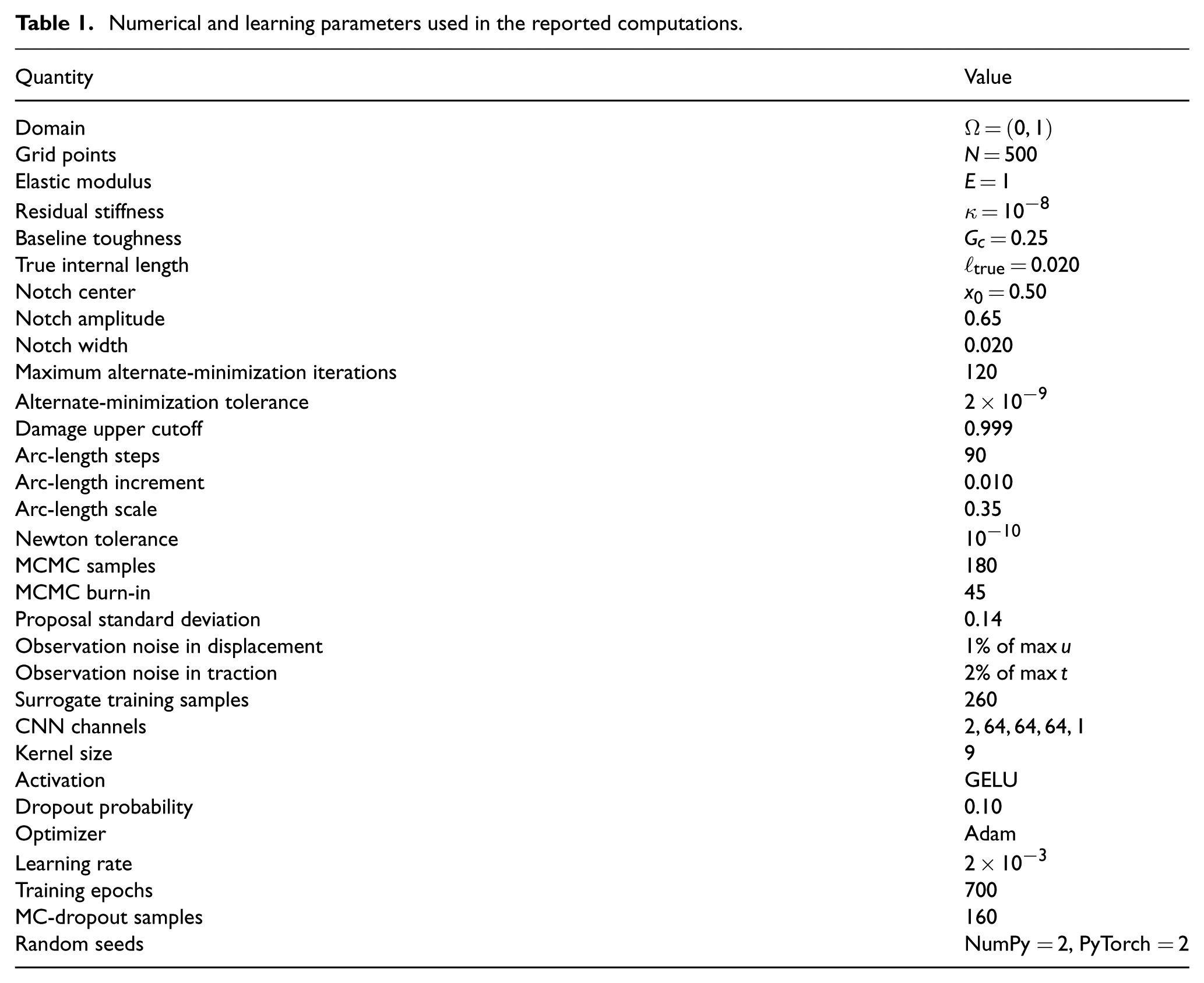
8.7. Implementation details and reproducibility

For reproducibility, we report here the numerical and learning parameters used in the computations. All simulations were performed on a 1D domain $Ω = (0, 1)$ discretized with $N = 500$ uniformly spaced grid points. The elastic modulus was set to $E = 1$ , the residual stiffness to $κ = 1 0^{- 8}$ , the baseline toughness to $G_{c} = 0.25$ , and the reference internal length to $ℓ_{true} = 0.020$ . Localization was induced by a Gaussian reduction of toughness centered at $x_{0} = 0.50$ , with amplitude 0.65 and width 0.020.

The deterministic AT2 solver used alternate minimization with maximum 120 staggered iterations and tolerance $2 \times 1 0^{- 9}$ . The damage variable was clipped to $d \leq 0.999$ to avoid complete stiffness loss. Arc-length continuation used 90 loading steps, arc-length increment $Δ s = 0.010$ , scaling parameter $c = 0.35$ , Newton tolerance $1 0^{- 10}$ , and a maximum of 60 Newton iterations.

Bayesian calibration of the internal length was performed using a log-space random-walk Metropolis–Hastings algorithm. The prior was log-normal with

\log ℓ \sim N (\log (0.02), 0.3 5^{2}) .

Synthetic observations were generated from 10 points sampled along the computed traction–displacement path. Gaussian noise was added to both displacement and traction, with standard deviations

σ_{u} = 0.010 \max_{i} u_{i}, σ_{t} = 0.020 \max_{i} t_{i} .

The Markov chain Monte Carlo (MCMC) chain used 180 samples with 45 burn-in samples and a log-space proposal standard deviation of 0.14. The reported acceptance rate was monitored directly from the chain.

For field-level UQ, the surrogate was trained on 260 synthetic samples generated by the deterministic AT2 solver. The training parameters were sampled as

ℓ \sim U (0.012, 0.05), t \sim U (0.85 t_{\min}, 1.05 t_{\max}),

where $t_{\min}$ and $t_{\max}$ were obtained from the deterministic path. The surrogate input consisted of two channels, one for ℓ and one for t, each repeated over the spatial grid. The output was the damage field $d (x)$ .

The surrogate architecture was a 1D CNN with MC-dropout:

2 \to 64 \to 64 \to 64 \to 1

channels, kernel size 9, padding 4, GELU activations, and dropout probability $p = 0.10$ after each hidden convolutional layer. The network was trained using the Adam optimizer with a learning rate $2 \times 1 0^{- 3}$ for 700 epochs, using mean-square error loss,

L_{MSE} = \frac{1}{N_{train}} \sum_{j = 1}^{N_{train}} ∥ S_{ϕ} (ℓ_{j}, t_{j}) - d_{j} ∥_{L^{2} (0, L)}^{2} .

MC-dropout was retained at inference time. For each test input, 160 stochastic forward passes were used to estimate the predictive mean, variance, and $95 %$ pointwise credible intervals.

The implementation used fixed random seeds, namely numpy.random.seed(2) and torch. manual_seed(2), to make the synthetic data generation, MCMC initialization, and surrogate training reproducible (Table 1).

Table 1.

Numerical and learning parameters used in the reported computations.

Quantity	Value
Domain	$Ω = (0, 1)$
Grid points	$N = 500$
Elastic modulus	$E = 1$
Residual stiffness	$κ = 1 0^{- 8}$
Baseline toughness	$G_{c} = 0.25$
True internal length	$ℓ_{true} = 0.020$
Notch center	$x_{0} = 0.50$
Notch amplitude	0.65
Notch width	0.020
Maximum alternate-minimization iterations	120
Alternate-minimization tolerance	$2 \times 1 0^{- 9}$
Damage upper cutoff	0.999
Arc-length steps	90
Arc-length increment	0.010
Arc-length scale	0.35
Newton tolerance	$1 0^{- 10}$
MCMC samples	180
MCMC burn-in	45
Proposal standard deviation	0.14
Observation noise in displacement	$1 %$ of $\max u$
Observation noise in traction	$2 %$ of $\max t$
Surrogate training samples	260
CNN channels	$2, 64, 64, 64, 1$
Kernel size	9
Activation	GELU
Dropout probability	0.10
Optimizer	Adam
Learning rate	$2 \times 1 0^{- 3}$
Training epochs	700
MC-dropout samples	160
Random seeds	NumPy $= 2$ , PyTorch $= 2$

8.8. MC-dropout as approximate predictive uncertainty

Dropout remains active during inference. Repeated stochastic forward passes generate

D^{(s)} (x) = S_{ϕ^{(s)}} (θ^{⋆}, a^{⋆}), s = 1, \dots, S .

We estimate:

\bar{D} (x) = \frac{1}{S} \sum_{s = 1}^{S} D^{(s)} (x),

Var [D] (x) = \frac{1}{S - 1} \sum_{s = 1}^{S} {(D^{(s)} (x) - \bar{D} (x))}^{2} .

Hence, the numerical uncertainty bands reported later correspond to predictive uncertainty generated by MC-dropout.

This should be interpreted as a scalable approximate Bayesian surrogate methodology, not as an exact substitute for the ELBO-based variational posterior in the previous section.

8.9. Why this implementation is scientifically appropriate

The use of a CNN + MC-dropout benchmark surrogate is scientifically justified for three reasons.

First, the current numerical study is 1D and smooth; therefore, the expressive advantages of a full FNO are not essential.

Second, the paper’s validated scientific question concerns identifiability under weakly informative data, not architecture benchmarking.

Third, the lightweight surrogate allows thousands of forward evaluations required for MCMC calibration at negligible cost.

Thus, the chosen implementation is a deliberate proof-of-concept realization of the broader framework rather than a contradiction of it.

8.10. Posterior prediction and field maps

The parameter posterior $p (θ ∣ D)$ quantifies global calibration uncertainty. The surrogate predictive variance quantifies field-level uncertainty. Combined, they provide:

uncertainty in inferred internal length scale;

uncertainty in reaction predictions;

spatial uncertainty concentration near evolving damage zones.

This separation between parameter uncertainty and field uncertainty is one of the central methodological outputs of this paper.

8.11. Summary of methodological consistency

To avoid any ambiguity, the methodology used in this paper can be summarized as follows:

Component	Role in the present manuscript
AT2 solver	deterministic ground truth
Metropolis–Hastings	parameter posterior sampling
CNN surrogate	fast operator approximation
MC-dropout	predictive uncertainty approximation
ELBO Bayesian framework	general future-ready formulation
FNO architecture	canonical scalable extension

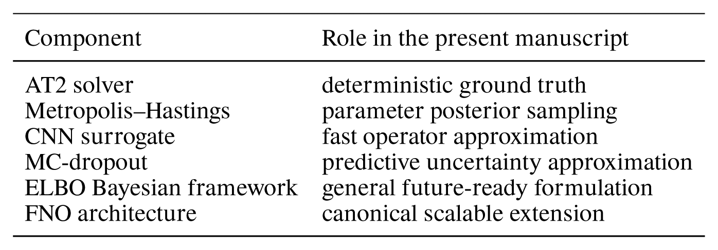
The manuscript therefore now consistently distinguishes between the general Bayesian operator-learning framework and the specific benchmark implementation used for the reported numerical evidence.

9. Results and discussion

This section reports the deterministic phase-field response together with the associated inverse and operator-learning results within a unified statistical–mechanical perspective. The numerical experiments specialize the general framework to the incremental irreversible AT2 formulation introduced in the computational discussion. All reported computations correspond to monotone pre-critical loading paths without observed limit points. Accordingly, the purpose of the present numerical study is not post-peak branch tracking, but rather the investigation of parameter identifiability under weakly informative global data. The surrogate results presented here are obtained using a CNN trained by mean-square regression and evaluated through MC-dropout for predictive UQ. These computations are intended as a benchmark realization of the broader Bayesian operator-learning framework developed earlier, rather than as a full Bayesian FNO implementation. Throughout, the numerical observations are interpreted through the structure of the AT2 functional and the sensitivity of the induced solution operator with respect to the internal length ℓ.

9.1. Deterministic AT2 response under arc-length continuation

We consider the 1D AT2 functional on $Ω = (0, L)$ with scalar phase-field damage $d \in [0, 1]$ and displacement u. The constitutive degradation is governed by

\begin{matrix} g (d) = {(1 - d)}^{2} + κ, \end{matrix}

(55)

where $κ ≪ 1$ is a residual-stiffness parameter ensuring a strictly positive tangent modulus.

9.1.1. Global traction–displacement response

Under traction control, the boundary traction is parametrized by a load factor λ as

\begin{matrix} t (λ) = λ T_{0} . \end{matrix}

(56)

For a fixed damage field $d (x)$ , the 1D equilibrium equation implies a constant axial force,

\frac{d}{dx} (g (d) E u^{'} (x)) = 0 ⟹ g (d (x)) E u^{'} (x) = t (λ),

so that the end displacement is obtained by quadrature:

\begin{matrix} u (L; λ, d) = \int_{0}^{L} \frac{t (λ)}{E g (d (x))} dx = \int_{0}^{L} \frac{λ T_{0}}{E g (d (x))} dx . \end{matrix}

(57)

Appendix Figure 1 shows the resulting global traction–displacement curve traced by arc-length continuation. Over the explored loading range, the path is monotone and close to linear, with no evidence of a limit point or snap-back. Mechanically, this indicates that the computed states remain on a stable, pre-critical branch in which the phase-field does not induce a sufficiently strong degradation to trigger a loss of incremental stiffness. In this regime, the arc-length procedure is not merely a numerical convenience: it provides a robust path-following mechanism that remains valid if the system later enters a post-peak domain, while here it confirms that the selected parameters do not drive the specimen into unstable crack growth.

9.1.2. Energy decomposition

To quantify how the response partitions between stored bulk energy and fracture regularization, we evaluate the AT2 energy

\begin{matrix} E (u, d) = \int_{0}^{L} g (d) ψ_{0} (u^{'}) dx + \int_{0}^{L} G_{c} (x) (\frac{d^{2}}{2 ℓ} + \frac{ℓ}{2} {(d^{'})}^{2}) dx, \end{matrix}

(58)

with the undamaged strain-energy density

\begin{matrix} ψ_{0} (u^{'}) = \frac{1}{2} E {(u^{'})}^{2} . \end{matrix}

(59)

The first integral in (58) defines the bulk contribution,

\begin{matrix} E_{bulk} (u, d) = \int_{0}^{L} g (d) ψ_{0} (u^{'}) dx, \end{matrix}

(60)

while the second defines the fracture regularization,

\begin{matrix} E_{frac} (d) = \int_{0}^{L} G_{c} (x) (\frac{d^{2}}{2 ℓ} + \frac{ℓ}{2} {(d^{'})}^{2}) dx . \end{matrix}

(61)

Appendix Figure 2 displays $E_{bulk}$ and $E_{frac}$ along the traced equilibrium path. The response is dominated by $E_{bulk}$ , whereas $E_{frac}$ increases only mildly and remains comparatively small. Importantly, the curves do not exhibit the energetic transfer typically associated with unstable crack advance, where a rapid growth of $E_{frac}$ accompanies a release of bulk energy. This energetic signature is fully consistent with the absence of a peak load in Appendix Figure 1 and confirms that the computed evolution remains diffuse rather than transitioning into a sharp localization event.

9.1.3. Damage localization evolution

Appendix Figures 3 to 8 report representative damage profiles $d (x)$ along the loading sequence. Damage initiates at the imposed imperfection (notch) located at $x = x_{0}$ and gradually amplifies as λ increases. However, the profiles remain smooth and the maximum damage stays well below unity, so that the system does not develop a fully formed crack within the simulated range. The finite width of the localization zone is governed by the internal length ℓ, as encoded in the gradient term of (58). In particular, the regularization penalizes sharp gradients through $\int_{0}^{L} G_{c} (x) \frac{ℓ}{2} {(d^{'})}^{2} dx$ , preventing mesh-scale localization and selecting a characteristic damage-band thickness proportional to ℓ. The observed profiles therefore provide a direct a posteriori consistency check of the variational implementation: the computed fields exhibit the expected regularization-induced smoothness and localization length while remaining on a stable branch.

9.2. Bayesian identification of the internal length

We now quantify how informative the global response is for identifying the internal length ℓ. The central issue is that, in a pre-critical regime where d is small, the mapping from ℓ to global reaction data is weak, and Bayesian posteriors may be dominated by the prior and measurement noise.

9.2.1. Synthetic data and inverse problem formulation

Synthetic observations are generated from the deterministic solver and perturbed by additive Gaussian noise in order to emulate experimental uncertainty. Appendix Figure 9 summarizes the calibration data and the resulting Bayesian sampling behavior.

Denoting by $D$ the set of measured pairs,

\begin{matrix} D = {(u_{i}, t_{i})}_{i = 1}^{N_{obs}}, \end{matrix}

(62)

The black curve in Appendix Figure 9 represents the deterministic traction–displacement relation obtained from the AT2 solver, while the blue markers correspond to the noisy observations used for parameter inference. The measurements remain closely aligned with the deterministic curve and display only small stochastic deviations reflecting measurement uncertainty. The data exhibit an almost perfectly monotone and nearly linear relation between traction t and end displacement $u (L)$ over the explored loading interval.

This behavior reflects the fact that the phase-field damage remains small along the computed branch, so that the degradation function $g (d)$ remains close to unity and the global response is dominated by elastic stiffness. In this regime, the forward relation between t and $u (L)$ is well approximated by the linear elastic relation

t \approx \frac{E}{L} u (L) .

Consequently, the calibration data contain only weak information about the internal length parameter ℓ, anticipating the practical nonidentifiability observed in the Bayesian inference results.

We infer ℓ through Bayes’ rule,

\begin{matrix} p (ℓ ∣ D) \propto p (D ∣ ℓ) p (ℓ), ℓ > 0, \end{matrix}

(63)

with a log-normal prior $p (ℓ)$ . The likelihood $p (D ∣ ℓ)$ is constructed by evaluating the forward map $ℓ \mapsto t (u; ℓ)$ through the arc-length solver and comparing the predicted and observed tractions at the measured displacements.

9.2.2. MCMC trace, posterior concentration, and pre-critical nonidentifiability

Before discussing Appendix Figures 10 to 12, we clarify the uncertainty sources represented in the reported results. Two distinct mechanisms arise in the present framework: (1) parameter uncertainty associated with the posterior distribution of the internal length scale ℓ and (2) surrogate epistemic uncertainty associated with the learned neural approximation.

Appendix Figures 10 and 11 concern the first mechanism only, since they report MCMC sampling results for ℓ. Appendix Figure 12 propagates posterior samples of ℓ through the deterministic forward solver and therefore represents parameter-induced predictive uncertainty in the global traction–displacement response.

By contrast, the field-level shaded bands reported elsewhere in the manuscript and obtained through MC-dropout correspond to surrogate epistemic uncertainty at fixed input parameters. They do not yet represent the fully propagated joint posterior that would arise from simultaneously sampling both ℓ and surrogate parameters.

Appendix Figure 10 displays the Metropolis–Hastings trace of the sampled internal length parameter ℓ. Starting from an initial value larger than the true parameter, the Markov chain rapidly relaxes toward smaller values during an initial burn-in phase. After approximately 40 iterations, the samples fluctuate within a quasi-stationary region, indicating that the chain has entered a stable sampling regime for the posterior distribution.

Despite this apparent stabilization, the sampled values remain concentrated in a range significantly below the true parameter value $ℓ_{true} = 0.02$ . In particular, the chain explores values approximately between $ℓ \approx 0.006$ and $ℓ \approx 0.012$ , suggesting that the likelihood provides only weak information about the true internal length under the present loading conditions.

This behavior becomes clearer when examining the posterior distribution shown in Appendix Figure 11. The histogram represents the empirical approximation of the posterior density $p (ℓ ∣ D)$ obtained from the MCMC samples, while the dashed vertical line indicates the true parameter value used to generate the synthetic data. The posterior mass is concentrated in a region significantly below $ℓ_{true}$ , and the true value lies outside the highest-density region of the posterior. Rather than indicating a failure of the sampling procedure, this discrepancy reflects a fundamental limitation of the available data: the global traction–displacement observations do not contain sufficient information to uniquely identify ℓ in the present regime.

The origin of this practical nonidentifiability can be understood analytically by examining the forward response in the limit of small damage. When the phase-field variable satisfies $d (x) ≪ 1$ uniformly on $(0, L)$ , the degradation function (55) satisfies

g (d) = 1 + O (d) .

Substituting this approximation into the displacement relation (57) yields

\begin{matrix} u (L; λ, d) = \int_{0}^{L} \frac{λ T_{0}}{E} (1 + O (d)) dx = \frac{λ T_{0} L}{E} + O (λ \int_{0}^{L} d (x) dx) . \end{matrix}

(64)

Combining (56) and (64) therefore gives, to leading order,

\begin{matrix} t = λ T_{0} \approx \frac{E}{L} u (L) . \end{matrix}

(65)

Equation (65) shows that, in the pre-critical regime where damage remains small, the global traction–displacement relation is essentially indistinguishable from the purely elastic response. Since the internal length ℓ enters the forward model primarily through the spatial structure of the damage field $d (x)$ , its influence on the global displacement $u (L)$ appears only through higher-order corrections. As a consequence, the likelihood function becomes nearly flat with respect to ℓ over a substantial parameter range.

This explains the numerical observations in Appendix Figures 9 to 11. The nearly linear traction–displacement data in Appendix Figure 9 provide only weak sensitivity to the internal length parameter, which leads the MCMC chain in Appendix Figure 10 to explore a broad region of parameter space. The resulting posterior distribution in Appendix Figure 11 is therefore dominated by prior assumptions and noise realizations rather than by strong information from the data, illustrating the practical nonidentifiability of ℓ in the present loading regime.

9.2.3. Posterior predictive response and field-level uncertainty

Appendix Figure 12 reports the posterior predictive traction–displacement relation obtained by propagating posterior samples of ℓ through the deterministic solver. The predictive mean essentially coincides with the deterministic response, and the credible band remains narrow. This is consistent with (65): in the pre-critical regime, global observables are well constrained even though ℓ itself is not. Stated differently, the inverse problem is ill-conditioned with respect to ℓ but not with respect to predicting the global curve on the explored branch.

For clarity, we distinguish two uncertainty mechanisms in the manuscript: parameter uncertainty associated with the posterior distribution of ℓ, and surrogate epistemic uncertainty associated with the learned neural approximation. Appendix Figure 12 concerns only the first mechanism, since the displayed band is obtained by propagating posterior samples of ℓ through the deterministic forward solver.

By contrast, the field-level uncertainty bands reported later in Appendix Figures 10 to 12 for spatial damage predictions correspond to MC-dropout uncertainty at fixed inputs and therefore quantify surrogate epistemic uncertainty rather than the full joint posterior obtained by simultaneously propagating uncertainty in ℓ and in the surrogate parameters. A complete combination of both uncertainty sources is a natural next step but lies beyond the scope of the present benchmark study.

This distinction is important for interpreting the numerical evidence. The current results validate that global response prediction may remain accurate despite weak identifiability of ℓ, while surrogate uncertainty tends to concentrate in mechanically active regions of the evolving damage field.

9.3. Bayesian neural-operator field posterior

We next move beyond global observables and quantify uncertainty at the field level. The objective is to learn a surrogate for the parametric solution map and to compute spatially resolved posterior uncertainty, which can concentrate where the operator is most sensitive, namely near localization zones.

9.3.1. Posterior mean and credible band

A neural-operator surrogate is trained to approximate the mapping

\begin{matrix} (ℓ, t) ⟼ d (\cdot), \end{matrix}

(66)

where $d (\cdot)$ denotes the damage field on Ω. Keeping dropout active at inference time yields MC samples that approximate a field-level posterior predictive distribution. Appendix Figure 13 shows the posterior mean and the $95 %$ credible band. The band is markedly wider in the neighborhood of the notch, reflecting the fact that the nonlinear coupling between degradation and equilibrium concentrates the sensitivity of d to parametric perturbations and surrogate uncertainty in that region.

9.3.2. Posterior variance localization

The spatial structure of uncertainty is further resolved by the pointwise posterior variance,

\begin{matrix} Var [d (x)] . \end{matrix}

(67)

As shown in Appendix Figure 14, $Var [d (x)]$ concentrates near $x = x_{0}$ , i.e., where the history field driving damage is largest and where the solution operator exhibits its strongest nonlinearity. In contrast, far-field regions remain close to the undamaged state and display negligible variance. This localization of uncertainty is a signature of operator sensitivity rather than observation noise alone: even when global observables are stable and nearly deterministic, the internal fields can retain highly structured epistemic uncertainty.

9.3.3. Pointwise posterior distributions

Appendix Figure 15 compares pointwise posterior distributions of $d (x)$ at the notch and away from it. Near $x_{0}$ , the distribution is broader and mildly non-Gaussian, consistent with the nonlinear saturation effects encoded by $g (d)$ and the irreversibility constraint. In the far field, the posterior collapses near $d ≃ 0$ , producing sharply concentrated distributions. Taken together, Appendix Figures 13 to 15 demonstrate that field-level inference exposes information that is invisible to global curves, in particular the spatial pattern of sensitivity and uncertainty induced by nonlocal regularization.

9.4. Theoretical discussion: Bayesian operator learning and identifiability

We now interpret the numerical findings through the lens of operator sensitivity and identifiability. The key point is that the AT2 model induces a nonlinear solution operator whose sensitivity to ℓ is regime-dependent: it is small on stable, pre-critical branches and can increase dramatically near bifurcation.

9.4.1. Nonlocal operator sensitivity

Let $R (d; λ, ℓ)$ denote the residual of the Euler–Lagrange equation for the damage field associated with (58) (including irreversibility handled via a history field). The induced solution operator can be viewed as

\begin{matrix} G_{ℓ} : (λ, G_{c}) ⟼ d (\cdot), \end{matrix}

(68)

defined implicitly by

\begin{matrix} R (d; λ, ℓ) = 0 . \end{matrix}

(69)

Assuming that the linearization $\partial_{d} R$ is invertible at a given state, the implicit function theorem yields the Fréchet sensitivity

\begin{matrix} \frac{∂d}{∂ℓ} = - {(\frac{\partial R}{∂d})}^{- 1} \frac{\partial R}{∂ℓ} . \end{matrix}

(70)

On a stable pre-critical branch, $\partial_{d} R$ is uniformly coercive and $\partial_{ℓ} R$ acts only through the regularization terms; consequently, the sensitivity (70) is small in norm, which explains the weak dependence of the global reaction curve on ℓ observed in Appendix Figures 10 to 12.

9.4.2. Fisher information and observable-level identifiability

Observable-level identifiability for ℓ is controlled by the Fisher information associated with the likelihood in (63). Writing $t (u_{i}; ℓ)$ for the model-predicted traction evaluated at $u_{i}$ , and assuming Gaussian observation noise with variance $σ^{2}$ , the log-likelihood takes the form

\log p (D ∣ ℓ) = - \frac{1}{2 σ^{2}} \sum_{i = 1}^{N_{obs}} (t_{i} - t (u_{i}; ℓ))^{2} + const.

Hence, the Fisher information is

\begin{matrix} I (ℓ) = E [{(\frac{\partial}{∂ℓ} \log p (D ∣ ℓ))}^{2}] = \frac{1}{σ^{2}} \sum_{i = 1}^{N_{obs}} {(\frac{∂t (u_{i}; ℓ)}{∂ℓ})}^{2}, \end{matrix}

(71)

where the expectation is taken with respect to the observation noise. In the pre-critical regime, (65) implies $\partial_{ℓ} t (u_{i}; ℓ) \approx 0$ , and thus, $I (ℓ)$ is small; the posterior cannot concentrate around $ℓ_{true}$ from global traction–displacement data alone. This explains why the posterior in Appendix Figure 11 is biased away from $ℓ_{true}$ despite the accurate posterior predictive curve in Appendix Figure 12.

9.4.3. Operator-level versus observable-level uncertainty

The preceding argument concerns only a scalar observable. In contrast, field predictions retain localized sensitivity even when global responses appear insensitive. In particular, the mapping (66) can respond sharply near $x = x_{0}$ because the local damage evolution is driven by concentrated history and the regularization balances ℓ-dependent gradient penalties against energetic driving. Bayesian operator learning targets a distribution over maps of the type (66); symbolically,

\begin{matrix} G_{θ} \sim p (G ∣ D), \end{matrix}

(72)

so that posterior predictive uncertainty becomes a spatially structured field. The variance localization observed in Appendix Figure 14 is therefore the field-level counterpart of the sensitivity structure encoded by (70): uncertainty concentrates precisely where the inverse of the linearized residual operator amplifies parametric perturbations.

9.5. Instability regime and snap-back behavior

Although the reported computations remain on a stable branch, it is useful to clarify how instability and snap-back modify both mechanics and identifiability. In nonlocal damage and phase-field fracture, loss of stability is associated with a degeneracy of the second variation of the energy, which simultaneously enhances parameter sensitivity.

9.5.1. Peak load condition in traction control

The global relations (56) and (57) define a parametric curve $λ \mapsto (u (L; λ), t (λ))$ . Differentiating (57) with respect to λ and using the λ-dependence of d yields

\begin{matrix} \frac{du (L)}{dλ} = \int_{0}^{L} \frac{T_{0}}{E g (d)} dx - \int_{0}^{L} \frac{λ T_{0}}{E} \frac{g^{'} (d)}{g {(d)}^{2}} \frac{∂d}{∂λ} dx . \end{matrix}

(73)

A limit point of the global path occurs when the incremental compliance vanishes, i.e.,

\begin{matrix} \frac{du (L)}{dλ} = 0, \end{matrix}

(74)

which is equivalent to $dt ∕ du (L) = 0$ since $t = λ T_{0}$ . Combining (73) and (74) shows that a peak load is reached when the damage-sensitivity term balances the purely elastic compliance term:

\begin{matrix} \int_{0}^{L} \frac{λ T_{0}}{E} \frac{- g^{'} (d)}{g {(d)}^{2}} \frac{∂d}{∂λ} dx = \int_{0}^{L} \frac{T_{0}}{E g (d)} dx, \end{matrix}

(75)

where $- g^{'} (d) = 2 (1 - d) > 0$ for $d < 1$ . The identity (75) emphasizes that instability is driven by the amplification of $\partial_{λ} d$ in the localization region: once damage evolves rapidly with loading, the effective incremental stiffness can vanish or become negative, producing snap-back.

9.5.2. Second variation, bifurcation, and loss of coercivity

Stability of a critical point of $E$ is determined by the second variation. Let $(u, d)$ be a stationary point of (58) (ignoring irreversibility for the purpose of the local bifurcation argument) and consider admissible variations $(δu, δd)$ . The second variation can be written in the canonical quadratic form

\begin{matrix} \begin{matrix} δ^{2} E (u, d) [δu, δd] & = \int_{0}^{L} g (d) E {(δ u^{'})}^{2} dx + \int_{0}^{L} g^{″} (d) ψ_{0} (u^{'}) {(δd)}^{2} dx \\ + \int_{0}^{L} G_{c} (x) (\frac{1}{ℓ} {(δd)}^{2} + ℓ {(δ d^{'})}^{2}) dx + 2 \int_{0}^{L} g^{'} (d) E u^{'} δ u^{'} δd dx . \end{matrix} \end{matrix}

(76)

Loss of stability corresponds to the loss of positive definiteness (coercivity) of (76), i.e., the existence of a nontrivial mode $(δu, δd) \neq (0, 0)$ such that $δ^{2} E = 0$ . In operator terms, this is a zero-eigenvalue condition for the Hessian of $E$ , and it coincides with the loss of invertibility of $\partial_{d} R$ appearing in (70). Consequently, near bifurcation, the inverse in (70) becomes large, and the sensitivity of the solution map to parameters (including ℓ) is amplified.

9.6. Identifiability theory

We formalize the preceding discussion by distinguishing identifiability on stable branches from identifiability near instability. While the full AT2 evolution includes irreversibility and potentially nonsmooth updates, the core mechanism can be established at the level of the forward map induced by the equilibrium branch.

9.6.1. Definition of identifiability

Let $θ = ℓ$ be the parameter of interest and define the (scalar) forward map constructed from global data as

\begin{matrix} F (ℓ) = t (u (L); ℓ), \end{matrix}

(77)

where $t (\cdot; ℓ)$ denotes the traction predicted by the model along the computed equilibrium path and evaluated at the observed displacements.

Definition 9.1 (Local identifiability). The parameter ℓ is locally identifiable from the chosen observable if $F$ is locally injective, and, in particular, if

\begin{matrix} \frac{\partial F}{∂ℓ} \neq 0 at the parameter value of interest . \end{matrix}

(78)

9.6.2. Pre-critical nonidentifiability

Theorem 9.2 (Pre-critical nonidentifiability). Assume that the computed equilibrium states satisfy $d (x) = O (ε)$ uniformly on $(0, L)$ for some $ε ≪ 1$ . Then, the global traction–displacement relation satisfies

\begin{matrix} t = \frac{E}{L} u (L) + O (ε), \end{matrix}

(79)

and, in particular,

\begin{matrix} \frac{∂t}{∂ℓ} = O (ε) . \end{matrix}

(80)

Consequently, ℓ is not identifiable from global traction–displacement data at leading order in ε.

Proof 10. By (55), $g (d) = 1 - 2 d + d^{2} + κ = 1 + O (ε)$ uniformly. Substituting into (57) gives

u (L) = \int_{0}^{L} \frac{λ T_{0}}{E} \frac{1}{1 + O (ε)} dx = \frac{λ T_{0} L}{E} + O (ε \frac{λ T_{0} L}{E}) .

Solving for $λ T_{0} = t$ yields (79). Since ℓ enters the global response only through $d (\cdot)$ in this regime, the estimate (80) follows immediately from the $O (ε)$ correction. The identifiability statement then follows from Definition 9.1.

9.6.3. Identifiability enhancement near instability

Theorem 9.3 (Identifiability enhancement near a loss of stability). Assume that the equilibrium branch approaches a critical load at which the linearized damage operator $\partial_{d} R$ loses invertibility, i.e., there exists a nontrivial mode φ such that

\partial_{d} R (d_{c}; λ_{c}, ℓ) φ = 0 .

Then, the sensitivity operator in (70) is unbounded as $λ \to λ_{c}$ in the sense that

\begin{matrix} ∥ \frac{∂d}{∂ℓ} ∥ \to \infty as λ \to λ_{c}, \end{matrix}

(81)

provided $\partial_{ℓ} R (d_{c}; λ_{c}, ℓ)$ has a nonzero component along the adjoint nullspace of $\partial_{d} R$ . In particular, the observable sensitivity $\partial_{ℓ} t (u; ℓ)$ is amplified near $λ_{c}$ , improving identifiability from global data.

Proof 11. Let $L : = \partial_{d} R (d; λ, ℓ)$ and $r_{ℓ} : = \partial_{ℓ} R (d; λ, ℓ)$ . Whenever L is invertible, (70) gives $\partial_{ℓ} d = - L^{- 1} r_{ℓ}$ . As $λ \to λ_{c}$ , L loses invertibility and its smallest singular value $σ_{\min} (L)$ tends to zero. Hence,

∥ L^{- 1} ∥ \geq \frac{1}{σ_{\min} (L)} \to \infty .

If $r_{ℓ}$ has a nonzero projection onto the critical mode (more precisely, onto the adjoint nullspace), then $∥ L^{- 1} r_{ℓ} ∥$ diverges with $∥ L^{- 1} ∥$ , establishing (81). Since the traction response depends on d through (57) and the equilibrium relation, the amplification of $\partial_{ℓ} d$ propagates to $\partial_{ℓ} t (u; ℓ)$ , increasing Fisher information (71) and improving identifiability.

9.6.3.1. Remark

Theorem 9.3 formalizes the heuristic that localization and the proximity to bifurcation act as a “variance amplifier” for parametric inference: as the tangent operator approaches singularity, small changes in ℓ induce large changes in the field, which then become visible to observables.

9.7. Bayesian operator-learning perspective

We close by linking the previous sensitivity results to operator-level UQ. Bayesian operator learning aims at a posterior over mappings (66), as symbolically indicated in (72). In this setting, uncertainty in ℓ and surrogate/model error jointly induce uncertainty in $d (\cdot)$ . A first-order propagation argument yields, at each $x \in (0, L)$ ,

\begin{matrix} Var [d (x)] \approx {(\frac{∂d (x)}{∂ℓ})}^{2} Var [ℓ] + {Var}_{model} [d (x)], \end{matrix}

(82)

where ${Var}_{model}$ denotes epistemic uncertainty in the learned operator. In a pre-critical regime, Theorem 9.2 implies $\partial_{ℓ} d (x)$ is small and the first term in (82) is weak; nevertheless, ${Var}_{model} [d (x)]$ can remain spatially localized near the notch because approximation error and nonlinear coupling are concentrated where gradients and history effects are largest. Near instability, Theorem 9.3 predicts a sharp growth of $\partial_{ℓ} d$ , so that the parametric component of (82) can dominate and lead to pronounced variance concentration in the localization zone. This provides a mechanistic explanation for why operator-level Bayesian surrogates can display strongly nonuniform uncertainty maps even when global curves appear nearly deterministic.

9.8. Summary of findings

The deterministic computations confirm that the adopted AT2 implementation yields a smooth, length-scale-controlled localization band and a stable, monotone global response over the explored loading range. The Bayesian inversion based solely on traction–displacement data reveals that ℓ is practically nonidentifiable on this pre-critical branch, in agreement with the small-damage expansion in Theorem 9.2. In contrast, field-level Bayesian surrogate predictions expose a spatially structured uncertainty landscape that concentrates near the notch, consistent with localized operator sensitivity. Finally, the operator-sensitivity analysis clarifies why identifiability is expected to improve dramatically as the system approaches a loss of stability: near bifurcation, the inverse of the linearized damage operator amplifies parametric perturbations, increasing Fisher information and tightening the posterior.

10. Conclusion

This work developed a mathematically consistent Bayesian operator-learning framework for nonlocal damage mechanics, aimed at connecting variational regularization in strain-softening solids with modern UQ for parametric solution maps. Starting from an AT2-type gradient damage formulation, we recast the coupled equilibrium–damage problem as a nonlinear operator acting between Sobolev spaces. This perspective provides a unified language for deterministic analysis, surrogate approximation, and Bayesian inversion.

On the deterministic side, the formulation preserves the regularizing structure of gradient damage models through a Helmholtz-type contribution that introduces an internal length scale ℓ, selects a finite localization width, and suppresses pathological mesh dependence. In the numerical regime examined here, all reported computations were intentionally restricted to monotone pre-critical loading paths without observed limit points or snap-back. The computed responses remained smooth, damage stayed below full degradation, and the resulting profiles exhibited the expected diffuse-zone thickness controlled by ℓ. These observations provide internal consistency checks while emphasizing the physical interpretation of ℓ as a localization-scale parameter.

The principal validated contribution of the paper concerns parameter identifiability. We showed that, in stable pre-critical regimes, global traction–displacement data may be only weakly informative for the internal length scale. In this setting, the sensitivity of global observables to ℓ is small, the Fisher information may become nearly degenerate, and Bayesian posteriors can remain diffuse or strongly prior-influenced even when macroscopic curve fitting appears accurate. This mechanism was confirmed numerically through synthetic-data calibration experiments: materially distinct values of ℓ produced nearly indistinguishable global responses, while the inferred posterior remained broad or biased. The practical conclusion is therefore direct and important: accurate agreement with reaction curves does not by itself imply reliable calibration of nonlocal constitutive length scales.

The numerical results reported in Appendix Figures 10 to 12 constitute the clearest evidence for this conclusion. The MCMC traces and posterior distributions demonstrate weak identifiability of ℓ under monotone pre-critical loading, while the posterior predictive global response remains sharply constrained. In other words, the inverse problem is ill-conditioned with respect to parameter recovery but comparatively well-conditioned with respect to predicting the explored global response branch. This distinction is central for interpreting calibration studies in nonlocal damage mechanics.

Field-level UQ further reinforces this message. Even when scalar observables are weakly sensitive to ℓ, the mapping from parameters to damage fields retains spatially structured sensitivity near the developing localization zone. The learned surrogate therefore produces uncertainty bands that concentrate in mechanically active regions rather than being distributed uniformly. Such information is valuable for risk-aware prediction and for experimental design, since it identifies where additional local measurements would be most informative.

Beyond the benchmark studied here, the framework is modular and naturally extends to richer settings. It is compatible with generalized continuum damage models, gradient plasticity, porous fracture theories, and coupled multi-physics degradation problems whenever a stable variational or monotone operator structure is available. It also suggests calibration strategies based on richer observation operators, including mixed loading paths and field measurements capable of breaking parameter degeneracies that persist under global data alone.

Several limitations define the next stage of development. The present numerical demonstrations were intentionally restricted to a 1D benchmark so as to isolate identifiability mechanisms in the simplest controlled setting. A natural continuation is to investigate whether genuine post-peak instabilities, limit points, and snap-back branches enhance identifiability through sensitivity amplification. Additional priorities include multidimensional benchmarks with complex crack patterns, stronger fully Bayesian neural-operator implementations, and explicit treatment of model discrepancy arising from constitutive idealizations, uncertain boundary conditions, and structured experimental noise.

In summary, this paper establishes a rigorous route toward probabilistic nonlocal mechanics by combining gradient-damage regularization, surrogate operator learning, and Bayesian inference. The most strongly validated conclusion is that internal length scales may be intrinsically difficult to identify from global data in stable pre-critical regimes, even when global predictions appear highly accurate. By making this limitation explicit and by quantifying where uncertainty localizes in the associated fields, the present work provides a statistically defensible and mechanically grounded basis for future calibration of nonlocal damage and fracture models.

Footnotes

Appendix 1 ORCID iD

Koffi Enakoutsa

Funding

The authors received no financial support for the research, authorship, and/or publication of this article.

Declaration of conflicting interests

The authors declared no potential conflicts of interest with respect to the research, authorship, and/or publication of this article.

Notes

References

Bažant

Pijaudier-Cabot

. Nonlocal continuum damage, localization instability and convergence. J Appl Mech 1987; 55: 287–293.

Peerlings

RHJ

de Borst

Brekelmans

WAM

, et al. Gradient-enhanced damage for quasi-brittle materials. Int J Num Methods Eng 1996; 39: 3391–3403.

Jirásek

. Nonlocal models for damage and fracture: comparison of approaches. Int J Solids Struct 1998; 35(31–32): 4133–4145.

Francfort

Marigo

. Revisiting brittle fracture as an energy minimization problem. J Mech Phys Solids 1998; 46(8): 1319–1342.

Ambrosio

Tortorelli

. Approximation of functionals depending on jumps by elliptic functionals via t-convergence. Commun Pure Appl Math 1990; 43(8): 999–1036.

Bourdin

Francfort

Marigo

. Numerical experiments in revisited brittle fracture. J Mech Phys Solids 2000; 48(4): 797–826.

Amor

Marigo

Maurini

. Regularized formulation of the variational brittle fracture with unilateral contact: numerical experiments. J Mech Phys Solids 2009; 57(8): 1209–1229.

Miehe

Welschinger

Hofacker

. Thermodynamically consistent phase-field models of fracture: variational principles and multi-field FE implementations. Int J Num Methods Eng 2010; 83(10): 1273–1311.

Borden

Hughes

TJR

Landis

, et al. A higher-order phase-field model for brittle fracture: formulation and analysis within the isogeometric analysis framework. Comput Methods Appl Mech Eng 2012; 217–220: 77–95.

10.

Tanné

Bourdin

, et al. Crack nucleation in variational phase-field models of brittle fracture. J Mech Phys Solids 2018; 110: 80–99.

11.

Placidi

Barchiesi

dell’Isola

, et al. On a hemi-variational formulation for a 2D elasto-plastic-damage strain gradient solid with granular microstructure. Math Eng 2022; 5: 1–24.

12.

Placidi

Timofeev

Maksimov

, et al. Micro-mechano-morphology-informed continuum damage modeling with intrinsic 2nd gradient (pantographic) grain–grain interactions. Int J Solids Struct 2022; 254: 111880.

13.

Allena

Scerrato

Bersani

, et al. A bi-dimensional model bridging microdamage evolution and bone remodeling: a computational study on a human femur. Math Mech Complex Syst 2025; 13: 347–376.

14.

Minku

Scerrato

Bersani

, et al. A quasi-brittle strain-driven microdamage-informed remodelling approach for predicting proximal human femur damage and remodelling patterns. Math Mech Complex Syst 2026; 14: 205–228.

15.

Riks

. An incremental approach to the solution of snapping and buckling problems. Int J Solids Struct 1979; 15(7): 529–551.

16.

Crisfield

. An arc-length method including line searches and accelerations. Int J Num Methods Eng 1983; 19(9): 1269–1280.

17.

Stuart

. Inverse problems: a Bayesian perspective. Acta Numerica 2010; 19: 451–559.

18.

Kaipio

Somersalo

. Statistical and computational inverse problems. Applied Mathematical Sciences. Springer, 2005.

19.

Kennedy

O’Hagan

. Bayesian calibration of computer models. J R Stat Soc B 2001; 63(3): 425–464.

20.

Dashti

Stuart

. The Bayesian approach to inverse problems. arXiv 2013; 1302.6989.

21.

Scuro

Pinchuk

Castellano

, et al. Genetic algorithms applied to nonlinear analysis for the identification of masonry structures collapse mechanisms. Math Mech Complex Syst 2024; 12: 233–261.

22.

Kovachki

Azizzadenesheli

, et al. Fourier neural operator for parametric partial differential equations. In: International conference on learning representations (ICLR), virtual event, 3–7 May, 2021.

23.

Kovachki

Azizzadenesheli

Liu

, et al. Neural operator: learning maps between function spaces. J Mach Learn Res 2023; 24: 1–97.

24.

Jin

Pang

, et al. Learning nonlinear operators via DeepONet based on the universal approximation theorem of operators. Nat Mach Intell 2021; 3: 218–229.

25.

Gal

Ghahramani

. Dropout as a Bayesian approximation: representing model uncertainty in deep learning. Proc ICML 2016; 48: 1050–1059.

26.

Blundell

Cornebise

Kavukcuoglu

, et al. Weight uncertainty in neural networks. Proc ICML 2015; 37: 1613–1622.

27.

Lakshminarayanan

Pritzel

Blundell

. Simple and scalable predictive uncertainty estimation using deep ensembles. In: Advances in neural information processing systems (NeurIPS), vol. 30, Long Beach, CA, 4–9 December, 2017.