Estimating Implicit Marginal Tax Rates of Welfare Recipients across the US States

Abstract

This article provides a more accurate estimate of implicit marginal tax rates (IMTRs) faced by low-income households in all fifty states. Complications arising from multiple program participation, regional differences in wage regulations, and cost of living make former generalizations about representative low-income households in a state potentially problematic. Additionally, it is appropriate to account for differences in work requirements by choosing the relevant margin to estimate the IMTR, and these margins vary by state. This article is the first to consider these margins, and, indeed, the author finds significant variation of IMTRs for different states. One of biggest sources of variation is the structure of child care subsidies provisions and cost. However, changes made to initial assumptions causes the estimated rates to vary in unpredictable ways. Given this complicated and unpredictable nature of the variation, researchers should exercise caution when using estimated IMTRs to examine work incentives of welfare programs.

Keywords

marginal tax rates welfare low-income households

The literature on tax rates and, more specifically, marginal tax rates (MTRs), is vast. Taxation policies play an influential role in economic growth, income distribution, and labor participation rates. Additionally, interstate variance in taxation levels can heavily influence interstate differences in these variables as well as migration patterns among states. The study of MTRs typically involves the use of descriptive or empirical methods, and sometimes a combination of both approaches.

Empirical approaches are useful and informative but limited in that they generally use state aggregated data, providing aggregated results that may not be true for the case of an individual income well below or above the mean. In this article, I employ a descriptive method to analyze the implicit marginal tax rates (IMTRs) facing low-income households. Consideration of tax policies affecting this population are of particular importance given the aim of policy makers to reduce poverty while promoting employment and self-sufficiency. An optimal tax policy for low-income households will assist individuals in need while also not unduly discouraging employment. These tax structures are difficult to achieve given the availability of a wide range of benefit programs targeted at low-income households (e.g., Temporary Aid to Needy Families [TANF], Food Stamps, housing subsidies). The gain individuals receive from increasing earned income and through the Earned Income Tax Credit (EITC), are often offset in whole or in part by a reduction in benefits from these other assistance programs.

This shortcoming has not gone unnoticed in the literature. Several studies recognize the conflicting nature inherent in a simultaneous tax credit and benefit reduction (Acs et al. 1998; Wolfe 2002; Romich, Simmelink, and Holt 2007). These studies have illustrated the potentially high MTRs that low-income households may face. High rates appear to persist even after the passage of the 1996 Welfare Reform Act, which aim was to reduce the disincentives that arise when low-income households face the prospect of losing a large portion of benefits as they increase employment. Since the reform the number of households receiving assistance has fallen, but this is likely due to the time limits outlined in the reform rather than the result of an optimal “taxation policy” regarding the strategic reduction in benefits.

As noted by these previous studies, to accurately calculate the current effective MTR for low-income individuals, one must aggregate the benefits of applicable government assistance programs at different levels of earned income. The analysis becomes complicated quickly because receiving benefits from one program may affect qualification for benefits in other programs. These distortionary effects can vary significantly by state and program participation; consequently, generalizing the result of a calculation of an effective MTR for a representative household in a median state under typical scenarios may be limited in scope. In order to completely understand the work incentives—or disincentives—embedded in the 1996 reform one must not limit the analysis to hypothetical working scenarios in a few states.

The flexibility given by the implementation of TANF extends beyond benefit levels and time limits. It also allows states to impose different work requirements on those who are determined eligible to receive assistance. As a result, the researcher’s choice of marginal increase in hours worked depends upon the working rules in each state. A working scenario that is appropriate for the analysis of Pennsylvania, for example, may not be so for the analysis of New Jersey. In the former the recipient is required to immediately start working twenty hours per week. In the latter, the recipient must increase his or her working hours to forty per week. A more accurate and correct estimation of MTRs must account for these differences.

To my knowledge, this article is the first to use the variation in state work requirements to estimate, and compare, the implicit MTRs for all fifty states. In doing so, this article advances the understanding of work incentives that each state creates for those recipients who want to meet the work requirements established. I also estimate the relative “contribution” each program makes to the implicit MTR, and highlight the difficulties that arise when changing the characteristics of the representative household.

I find significant variation in implicit MTRs for those willing to meet/comply with all work requirements across states. For example, a mother with two young children attempting to comply with these work requirements faces an IMTR of 38.8 percent in South Dakota and −1.6 percent in Ohio. The calculated MTRs are also sensitive to changes in the assumptions about the representative household. If we simply change the assumption that this mother has two older children rather than two children under six, the IMTR for North Carolina drops to approximately 4.0 percent from 21 percent. This variation likely has a significant impact on many important economic considerations and should be considered by both researchers and policy makers. I detail the procedure to compute these rates so that policy analysis and future relevant literature may more accurately assess the effects of these rates.

The remainder of this article is organized as follows: Literature Review section discusses previous literature. Following, the section Means-Tested Programs and IMTRs describes the welfare programs in detail while The IMTR and Its Calculation section puts them within the context of IMTRs. The section IMTR By Component discusses some of the driving forces of IMTR variations and the section Analysis of Assumptions Using Selected States analyzes the effects of certain assumptions on certain programs and is followed by the Conclusion.

Literature Review

Previous studies focusing on estimating MTRs typically use one of two methods. Empirically, researchers have followed the approach developed by Koester and Kormendi (1989). Their method calculates the MTR by estimating the income elasticity of tax revenues, which allows for the estimation of MTRs for particular jurisdictions. Reed, Rogers, and Skidmore (2011) note that the method developed by Koester and Kormendi (1989) results in a single estimation of the MTR for an entire period, rendering the estimation not applicable for panel data analyses. Additionally, the method wrongly assumes a constant tax structure and the estimated MTRs are not specific to any individual jurisdiction’s tax rules. They generalize the method to correct for these shortcomings. In particular, they allow tax parameters to vary by jurisdiction and change over time. These estimation techniques rely on income and tax revenue data to estimate the MTR.¹ Reed, Rogers, and Skidmore (2011) estimate MTRs for all fifty states and different periods while allowing for state specific tax parameters. However, their estimates do not provide information on state MTRs for individuals in a particular income bracket since they are based on state aggregate data.

An alternative method to estimating MTRs is to construct an estimate using rules governing the households in question. This is particularly useful when considering low-income households who may qualify for various tax credits and assistance programs. When calculating the implicit MTR one must incorporate all of the relevant benefit formulas and tax credits the chosen representative household is assumed to face. These assumptions vary across studies. Romich, Simmelink, and Holt (2007) illustrate the effect of benefit reductions on the net income of low-income households using two different scenarios. One considers a household receiving Food Stamps and rent subsidies but no child care costs while the other considers child care costs but no Food Stamp or rent subsidies. In the first scenario, an increase of $500 in earned income resulted in a net increase of $50 while in the second, an increase in earned income resulted in a net decrease in income.

Romich, Simmelink, and Holt (2007) highlight that the implicit MTRs may vary significantly between households as a result of, among other things, program participation and family composition. In particular, MTRs are very steep when earnings increase to such an amount that they are no longer eligible for benefits (these are referred to as cliff points). Other studies have altered this analysis with respect to considering different periods, locations, representative household construction, and assumptions regarding program participation (Shaviro 1999; Wilson and Cline 1994; Ellwood and Liebman 2001; Wolfe 2002; Sammartino, Toder, and Maag 2002).

While most studies are constrained to a particular state or jurisdiction, Acs et al. (1998) attempt to capture interstate variation by considering twelve states. They calculate the MTR faced by a representative family earning the federal minimum wage ($5.15 at that time) and working part-time, full-time, or full-time at a $9.00 wage for each of the twelve states individually. They assume the family receives TANF benefits and Food Stamps in all scenarios, but separately consider the case of a family receiving child care or rent subsidies. Under all scenarios, it is assumed that the family files both state and federal tax returns, earning the EITC when eligible. These MTRs are of secondary importance in their analysis; they focus on the percentage increase in net income as a means to capture the wealth or income effect, rather than on the percentage change in net income as a ratio to the percentage change in earned income.² They argue that the states chosen represent all areas of the country and that the variation in their wealth measure captures the interstate variation in work incentives. The highest variation between states occurs at low-income levels and narrows at higher-income levels. However, their analysis does not account for either different minimum wages or different work requirements in different states. Presumably the hours it takes to earn a given income level, which will differ across states when states have differing minimum wages, will influence the degree of participation in the labor market. Not accounting for this factor may bias results. Additionally, difference in work requirements implies that, on one hand, MTRs should be calculated at different margins for different states and, second, that given the short time allowed to meet the work requirements, a distinction between MTRs at the extensive (labor participation) and intensive (increase in work hours) margins may be difficult. Different work requirements mean that a recipient’s choice of labor participation may clearly depend upon the required increase in hours per week (from a state of welfare approval where no work has been undertaken yet).

More recently, Holt and Romich (2007) argue that previous studies are informative, but limited, by their assumptions. When constructing the hypothetical household, they argue that the distribution of families participating in various programs must be taken into account. They use a unique administrative data set for low-income households in Wisconsin and calculate the MTR for various household structures, program participation, and levels of employment. They find that the percentage of eligible households participating in two or more programs is rather small and for the most part none participate in TANF. Additionally, the phasing out of welfare benefits that accompany an increase in work hours leads to effective MTRs much higher than the formal MTR schedule. In particular, they estimate the distribution of high MTRs across family types and find a significant percentage of families led by single mothers facing MTRs above 50 percent. This is higher than the MTR faced by the highest-earning group according to the state and federal tax schedules.

The use of administrative data makes their study unique in that they can estimate MTRs based on actual program participation and true income levels. However, their analysis is constricted to Wisconsin only. This may be troublesome for those interested in the work incentives under multiple program participation given that Wisconsin has a unique TANF benefit structure. With three different versions, the most popular of its TANF structures (W-2) cuts all cash benefits as soon as the individual starts working. This explains the very low TANF participation rate of in their data set. More generous states may have higher participation rates, implying the need for a more complete analysis that includes TANF and all other states.

I build upon their research by doing a comprehensive analysis of all fifty states that includes TANF and the programs observed in their data set. Since I do not have information on the income distribution of low-income individuals, I base my calculations on those who aim at meeting the state work requirements, an important feature of the states' welfare design that has been left out of the literature so far. I find that some states do indeed yield similarly high MTRs as those found by Holt and Romich (2007). However, there are many exceptions. For example, I find the MTR faced by a family headed by a single mother of two children to be as low as 1.1 percent for New Mexico and even negative for states such as Missouri and Delaware. This suggests that findings regarding MTRs with respect to one state should not be generalized to other states.

Additionally, by estimating the implicit MTRs for all fifty states, this article allows for direct comparison of tax policies and outcomes between states. Construction of an implicit MTR schedule for low-income families by state is complicated by the fact that different states have different minimum wage laws.³ A higher minimum wage law at the state level, for example, may result in some families becoming ineligible to receive federal benefits at a lower level of hours worked than an identical household in a neighboring state. This in turn may influence the level and type of economic activity undertaken by low-income households, and partially explain the variation in state level economic activity.

Analyses that aggregate the estimation to the federal level cannot consider these, and other, important implications of implicit MTRs. To my knowledge, this is also the first article to highlight the complications embedded in the calculation. In some cases minor changes in assumptions yield nontrivial changes to the estimated implicit MTR, implying that MTR estimations are not only very complicated to accurately calculate but also are very sensitive to the conditions faced by households. This sensitivity must be noted when drawing conclusions about the effect of the policies on labor force participation rates, given the extensive literature dedicated to the effects of means-tested programs on employment.

For instance, Garfinkel and Orr (1974) and Williams (1975) find that female labor participation rates are negatively influenced by the phase-out benefits of assistance programs. In contrast, Keane and Moffitt (1998) find that these resulting tax rates have modest impacts on labor supply, and Meyer (2002) finds that the effect of the Earned Income Credits are noticeable at the extensive margins but not at the intensive one.⁴ This article illustrates that using a national average of the implicit tax rates will not accurately describe the conditions faced by most low-income households. Additionally, even attempting to use the most consistent and thorough procedure for capturing the correct estimates may not produce the same implicit MTR, both in direction and magnitude, when changes are made in the assumptions. Given this potential ambiguity, the study of implicit MTRs remains a relevant discussion for those interested in the analysis of employment rates and levels for low-income individuals.

Means-Tested Programs and MTRs

The Personal Responsibility and Work Opportunity Reconciliation Act of 1996 reformed the welfare system with the objective of reducing welfare dependence and promote work among low-income households. Each state was given more freedom to modify cash benefit packages that were previously controlled by stricter federal rules. The power given to states was conditioned on certain federal guidelines, most notably lifetime time limits. The Act of 1996 aimed at transforming the cash-benefit program to make it a temporary safety net helping the very low-income individuals become self-sufficient.

While variation among states already existed for some programs, including the old Aid to Families with Dependent Children (AFDC), the 1996 reform formally established the states' new increased flexibility in experimenting with maximum cash benefits, benefit reduction rates (BRRs), earnings disregards, and even time limits that should not extend beyond sixty months. Under the new program (TANF), the federal government required states to have a certain percentage of families receiving benefits complying with strict work requirements (Acs et al. 1998; Meyer 2002).

To complicate matters further, analysts must also consider the availability and interactions among the different available programs. Since cash assistance may not be enough to alleviate economic hardship for a working parent, he or she may be obliged to participate in other programs such as Food Stamps (now known as SNAP), housing and child care subsidies, Women and Infant Care (WIC), and subsidized health care. In addition, low-income parents are eligible to claim tax credits and deductions to the tax system, which in most cases helps increase annual disposable income. However, most means-tested programs are designed in a way such that benefits are reduced as income increases. This in turn has the potential of creating high MTRs if benefits are reduced faster than the increase in earnings. Economists calculate this implicit MTR by calculating the ratio of the change in earned income to the change in disposable income (after benefits have been reduced and all tax credits and liabilities have been taken into account) and subtracting it from one: $I M T R = 1 - [Δ E a r n i n g s / Δ N e t I n c o m e] .$ Romich, Simmelink, and Holt (2007) point out that IMTRs for low-income individuals are usually steeper under the utilization of multiple programs. Yet, this may not always be the case. Not only do IMTRs depend on the number of programs used and the welfare rules in each particular state, but also on the particular assumptions about what is considered to be the hypothetical recipient. In this analysis I use the EITC, TANF, the cash value of Food Stamps SNAP, and child care subsidies. Tax liabilities include the federal and state income taxes, as well as the share of payroll taxes borne by the worker. The hypothetical welfare recipient is assumed to be a single mother with two children under the age of six.⁵ Other assumptions about this recipient will vary throughout the study in order to highlight the complications embedded in the estimation of these IMTRs across states.

The choice of programs is rather arbitrary since it varies from household to household. Consequently, IMTRs may vary on this margin as well. This analysis focuses on the work incentives provided by all the different states under the new federalism of welfare and TANF plays the central part of this analysis. Data for 2006 TANF recipients suggest that, on average, approximately 80 percent also receive Food Stamps (SNAP) and most of them participate in some kind of medical assistance program. Quantifying medical benefits under Medicaid/SCHIP is cumbersome, so I follow Acs et al. (1998) by not including them in the simulation.⁶ According to them, although tied to TANF, child care subsidies are only received by those that actually need it or would use it. However, due to quality concerns, mothers prefer to not take the benefit and leave their children with a family member. Additionally, these subsidies are theoretically “pegged” to actual costs, covering most of the needed child care expenses with the exception of some small copayments. In theory, assuming that mothers do make use of the program, subsidies should cover most of the costs and would not affect take home earnings and/or MTRs significantly. If subsidies schedules are not updated frequently, actual costs may be greater than the aid imposing a burden on the disposable income of a working mother. Different states also have different stipulations about the provision of the subsidy, affecting the calculations. I assume that single mothers do need the use of a caretaker, and thus apply for the benefit.

Previously mentioned studies analyzing MTRs provide detailed discussions about the insights of these programs. Hence, I only discuss them briefly.⁷

TANF

As mentioned, TANF replaced the AFDC. Under the program, recipients must get a job as soon as possible with a maximum unemployment time of two years. Initially only 25 percent of recipients had to participate in some kind of “work related activities” but by the fiscal year 2000, the requirement was a minimum of thirty hours per week in most states. These outlines are general and specific requirements vary by state. For example, some states define work activity as schooling, training, or skill development. Making allowances for educational programs, work hours required range from twenty in some states to forty in others. Even in states where there are no education/training allowances, they may require less hours per week for those mothers with children under the age of six. As a means-tested program, eligibility depends on income, assets, and the presence of dependent children under the age of eighteen (see also Lugalla 2005). Benefits are provided on a monthly basis, and receipt is based on income and work hour compliance in the previous month. TANF benefits are reduced as income increases, with states determining the pace at which they are phased out.

Food Stamps

Foods stamps (now SNAP) are provided by the US Department of Agriculture and eligibility guidelines are such that individuals eligible for TANF are generally eligible for food stamps. While some argue that this is an in-kind benefit rather than a cash transfer, others argue that it frees up money that households would otherwise allocate for food to be used elsewhere (Lugalla 2005). As such, it may be treated as a cash transfer. The benefit received depends on both income and housing costs, making some additional allowances for child care costs. Like TANF, the benefit value is decreases as income increases beyond certain levels. Even though these benefits are provided at the federal level, the actual benefit varies across states as it uses TANF as part of gross income and calculates house and child care allowances based on actual costs.

Child Care Subsidies

Child care subsidies funded by the federal Child Care and Development Fund (CCDF) and are closely tied to TANF. Like TANF, states have the flexibility to set income eligibility as well as copayments. Typically there a subsidy is provided when needed, and the amount depends on the number of children, type of child care, and income. This program is often considered as a key partner of TANF because of its goal of providing the resources parents may necessitate as they attempt to gaining work skills and/or experience and becoming self sufficient.

EITC

The EITC is a program created to exclusively incentivize work, providing tax incentives to low-income individuals. Individuals are required to work, and are able to claim the credit when they file for their tax refunds.⁸ Its structure is of particular interest to many researchers given its unique design. At very low-income levels, the credit increases (phases in) with increased earnings at a rate of 40 percent. This serves as an incentive to work more. In fact, the program has been found to be one of the main drivers of increases in the labor force participation of low income single mothers (Meyer and Rosembaum 2000, 2001). As earnings increase, benefits flatten out and eventually start falling at a rate of 21 percent (Romich, Simmelink, and Holt 2007). Some states have their own version of their EITC.

The IMTR and its Calculation

After choosing the relevant programs, making reasonable assumptions, and calculating the tax liabilities and benefit amounts for each of the chosen programs at different income levels, calculating the IMTR is straightforward. Tax liabilities are comprised of the payroll tax share borne by the worker, given that at very low levels of income federal taxes are nonexistent. Some states have income taxes, but these rates are typically zero for the household in question.

One complication when calculating MTRs for a given state or jurisdiction is defining the margins of interest. The researcher must decide whether it is appropriate to analyze marginal increases in income, or marginal increases in hours worked. Acs et al. (1998), for instance, choose four different scenarios: no work, part-time work at minimum wage, full-time work (thirty-five hours per week) at minimum wage, and full-time work at a higher than minimum wage. For all purposes, such scenarios are very informative and make intuitive sense, but are somewhat limited in their power to draw more generalizing conclusions. In fact, further investigation reveals that these MTRs are sensitive to the choice of scenario, yielding unpredicted results on occasion.

For this analysis, I chose to estimate IMTRs based on an increase the number of hours worked. This was done for three reasons. First, since this article is primarily concerned with the work incentives embedded in TANF, I focus on the income levels that capture the phase-out of benefits. In many states, an individual who works forty hours a week at the minimum wage is no longer eligible for TANF benefits. Hence, a scenario in which a full-time worker experiences an increase in income through an increase in wages leaves out the impact of TANF benefit reduction on MTRs. Also, the reform established that states must set work requirements as part of the work incentives, implying that welfare administrators are primarily concerned with promoting both work participation and effort—in the form of hours—before increasing the income of low-wage individuals. Second, in their effort to promote work, TANF allows recipients to occupy some of their time in educational activities. This implies that recipients are usually low-skilled individuals who need time to improve their skills before they are ready to work full-time or even higher wages.

A third reason, perhaps related to the preceding one, is to capture whether new eligible TANF recipients do or do not face the disincentives to work. As mentioned above, the EITC starts with a phase-in design that may offset the phasing-out of other benefits. To the extent that the increase in EITC is greater than the overall reduction of benefits, the individual will face a negative IMTR and will be incentivized to work the extra hours. For single mothers, this phase-in part of the EITC falls on mothers with no high-school diploma (Meyer 2002) with limited skills, low levels of income, and thus few if not zero hours of work.

Choosing a reasonable margin is an important part of the calculation but does not solve the complications about estimating accurate and generalizing results. Table 1 shows simulated IMTRs for four different states and different working-hour margins for a single mother of two children under six. The results suggest that even when focusing on hours, the IMTRs vary widely at both the extensive and intensive margins, depending on the chosen increase in working hours. Contrary to some previous calculations, the table also shows that IMTRs for such mother do not always increase with the number of programs included. In fact, some of those IMTRs are negative rather than high and positive, providing an incentive to work. In order to understand these complications and the source of changes in IMTRs across states, one must be necessarily careful in choosing the correct margin and number of programs. I rely on the TANF rules to simplify the marginal analysis and on previous studies for the programs of choice.

Table 1.

Implicit Marginal Tax Rates for Low-Income Mothers of Two Children under Six for Different Margins (percentage)

	Ten-hour increase				Part-time and full-time		Other extensive margins
State/Programs	0–10	10–20	20–30	30–40	0–20	20–40	0–30	0–40
Arizona
TANF only	9.4	37.7	11.2	−32.3	23.5	−10.5	19.4	6.5
TANF and SNAP	9.4	−32.3	13.0	−8.5	23.5	2.2	−32.4	12.9
TANF, SNAP, and care subsidy	9.4	37.7	26.0	26.9	23.5	26.5	24.4	25.0
Ohio
TANF only	−32.3	11.7	17.5	17.5	−10.3	3.6	−1.0	3.6
TANF and SNAP	−28.7	25.6	31.4	30.9	−1.6	65.6	9.4	14.8
TANF, SNAP, and care subsidy	−4.0	0.9	31.4	33.6	−1.6	32.5	9.4	15.5
Rhode Island
TANF only	−11.3	17.5	17.7	39.0	−93.8	28.4	8.0	15.7
TANF and SNAP	6.2	26.7	28.0	52.7	16.4	40.3	20.3	28.4
TANF, SNAP, and care subsidy	87.7	−54.8	28.0	55.5	−67.1	41.7	20.3	29.1
Virginia
TANF only	−32.3	17.5	−32.7	−32.3	−32.3	−32.5	−1.0	−32.4
TANF and SNAP	−32.3	26.7	−8.1	−3.6	−22.2	−5.8	9.4	−14.0
TANF, SNAP, and care subsidy	−18.4	−54.8	33.6	102.2	6.7	67.9	9.4	37.3

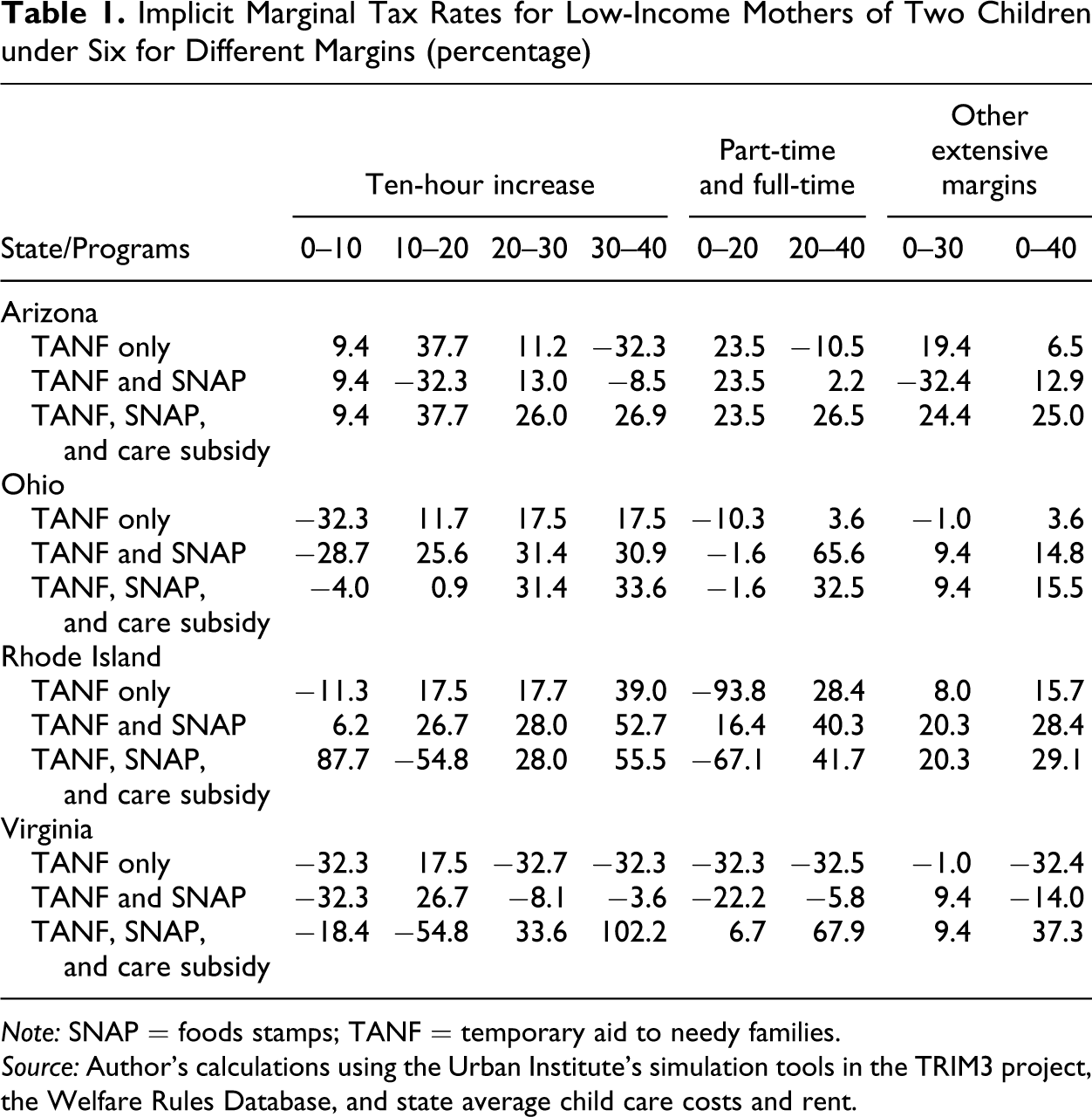
Note: SNAP = foods stamps; TANF = temporary aid to needy families.

Source: Author’s calculations using the Urban Institute’s simulation tools in the TRIM3 project, the Welfare Rules Database, and state average child care costs and rent.

One of the important changes in the reform was the introduction of work requirements. I argue that the calculation of these IMTRs needs to be conducted within this context, in order to correctly measure the incentives faced by welfare recipients wanting to comply with the stipulated working rules. In most states these requirements must be met immediately, while others allow a small grace period. In any case, recipients should try to comply soon after being approved for benefits, as states' funding from the federal government may be reduced if a certain percentage of recipients fail to comply. This implies an estimation of MTRs at the extensive margin that is heavily influenced by the required amount of hours—an intensive one. Moreover, since requirements are set at the state level and individuals in different states may meet work requirements at different intensive margins, researchers and policy makers must be wary of the risks of interpreting and comparing these IMTRs across states.

Figure 1 displays calculated MTRs for single mothers with two children under the age of six who are willing to comply with the state rules, under two sets of different assumptions. The simulations use minimum wages, median rent costs, and cost of child care for two children of age four for 2006. The benefit reduction calculation of TANF follows the rules obtained from the Welfare Rules Database (WRD) for 2005. Food Stamps calculations follow federal rules published in the website and child care copayment rules are from the 2005 CCDF state plans.⁹ Federal tax liability follows guidelines established on the Federal 1040 form while state liabilities are based on booklets. Families are assumed to take all tax credits and deductions for which they are entitled, including the assumption that all children are claimed as dependents. Furthermore, it is assumed that adults do not make contributions to tax-exempt vehicles such as a 401(K) or an Individual Retirement Account. No local taxes are included in the calculation.¹⁰ Income tax liabilities at both the federal and The state level are simulated through the Urban Institute’s TRIM3 simulation tool, and compared with simulations obtained from the NBER TAXSIM tool, finding little difference.

Figure 1.

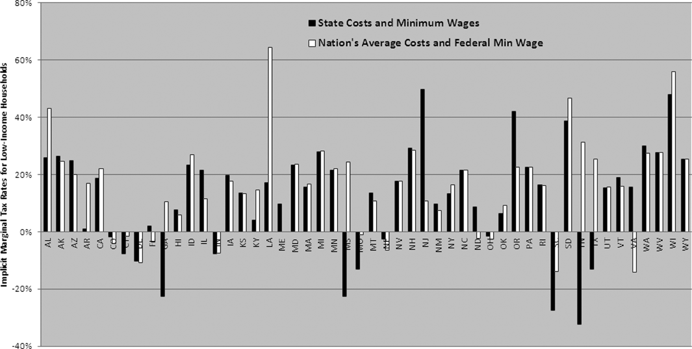
Implicit marginal tax rates (IMTRs) faced by low-income mothers with two children under the age of six for the year 2006

One of the IMTR series in Figure 1 displays results when the calculation assumes that all inputted values are the same for all states (e.g., federal minimum, nation’s average rent value, and the nation’s average child care cost). This allows us to see the variation in state IMTRs under full compliance when everything is assumed equal among states. As shown, there is a wide variation among states. This is partly due to the difference in TANF benefit rules and partly due to the TANF work requirement rules. Presumably, TANF and child care subsidies are set to reflect the cost of living in a given state. Thus, it is important to do the simulations using state specific wages and costs. The other series in Figure 1 depicts such a scenario. As shown, there is no clear pattern or consistency on the results from this simulation when compared to the first scenario. Not only are the magnitudes different, but in some cases they also have opposite signs. For instance, Florida had a positive IMTR in the first case, but a negative one under the one using state specifics. In theory, this is a welcomed result suggesting that Florida does indeed target the interaction among its programs such that it reflects state costs of living, while providing incentives to work. In contrast, Tennessee and Texas experience positive MTRs. In order to better understand the nature of such changes in IMTRs, it is necessary to look at the components and driving forces of such rates.

IMTR by Component

Disentangling the composition of MTRs is straight forward and useful for this type of analysis. Looking at the driving forces of each state’s IMTR provides further insights on how the programs impact the overall MTRs faced by low-income and uneducated mothers. To illustrate the composition of MTRs I simply reconstruct the formula for the IMTR provided above as follows,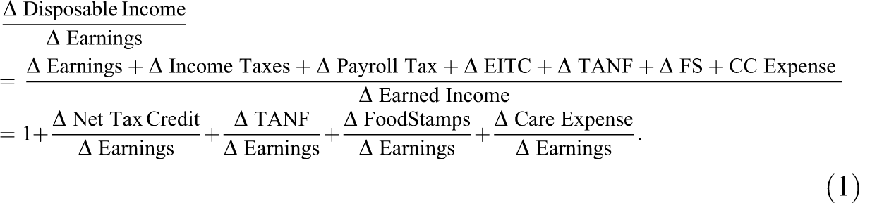

\frac{Δ D i s p o s a b l e I n c o m e}{Δ E a r n i n g s} = \frac{Δ E a r n i n g s + Δ I n c o m e T a x e s + Δ P a y r o l l T a x + Δ E I T C + Δ T A N F + Δ F S + C C E x p e n s e}{Δ E a r n e d I n c o m e} = 1 + \frac{Δ N e t T a x C r e d i t}{Δ E a r n i n g s} + \frac{Δ T A N F}{Δ E a r n i n g s} + \frac{Δ F o o d S t a m p s}{Δ E a r n i n g s} + \frac{Δ C a r e E x p e n s e}{Δ E a r n i n g s} .

such that

1 - \frac{Δ D i s p o s a b l e I n c o m e}{Δ E a r n e d I n c o m e} = - [\frac{Δ N e t T a x C r e d i t}{Δ E a r n i n g s} + \frac{Δ T A N F}{Δ E a r n i n g s} + \frac{Δ F o o d S t a m p s}{Δ E a r n i n g s} + \frac{Δ C a r e E x p e n s e}{Δ E a r n i n g s}]

where the first term in the right-hand side is always negative and will only change in cases where there is a state income tax. This is given that payroll tax rates are constant at 7.5 percent of every additional dollar earned, federal income taxes are nonexistent for these individuals and constant across states, and the phase-in portion of the EITC is constant at 40 percent of each additional dollar. The sign of the IMTR depends on whether the magnitude of the relative changes in the three programs with respect to additional earnings is greater than or less than the one of the tax change to earnings change ratio. If greater, the sign will be positive and there will be implicit taxation (e.g., the loss of additional gross earnings) and thus a disincentive to work more.

Tables 2 and 3 show the contribution of the three welfare programs to the IMTRs for the two scenarios for all fifty states under the given compliance rules. Both tables have been ranked by the magnitude of their IMTR. In both cases, there are some states in which the tax credits outweigh the effect of the benefit reductions resulting in negative IMTR. Table 2 allows us to look at the composition of MTRs under the hypothetical case in which all states were subject to the same minimum wage ($5.15) and same costs of living costs of living. The fact that some states have stricter work requirements does not necessarily translate into higher MTRs. Virginia, for example, requires that TANF recipients work thirty hours per week, with no allowance for educational training. Yet, the overall IMTR is negative. This is mostly due to the design of its TANF program. Under the state’s provision a family of three is eligible for a maximum monthly payment of $320 and a high income disregard. In most cases, the higher the disregard, the lower the overall TANF reduction at low levels of income. Indeed, as the Table 2 shows, given these characteristics, TANF benefits are not reduced at all even when work increases by as much as thirty hours per week. This is consistent with the results show in Table 3. However, child care costs in Virginia significantly above the national average, which implies that even when child care is received at an hourly rate, there is a significant increase in the amount of care expenses incurred by the mother.

Table 2.

Implicit Marginal Tax Rates Faced by Low-Income Mothers with Two Children under the Age of Six Using Federal Minimum Wages, and Nation Average Costs of Living for 2006

		Take-back rates corresponding to means-tested programs
State (min hour requirement)^a	IMTR (%)	TANF (%)	Food stamps/SNAP (%)	Net child care expenditures (%)
Virginia (30)	−14.2	0.0	16.7	1.3
South Carolina	−13.9	0.0	0.0	18.4
Delaware	−10.8	0.0	7.2	14.3
Indiana	−7.4	25.1	0.7	0.0
Nebraska	−6.5	17.7	8.1	0.0
Colorado (22)	−4.0	14.8	6.3	7.2
Florida	−3.6	0.2	0.9	27.6
Ohio	−2.7	5.2	7.4	17.0
North Dakota	−2.2	9.9	20.2	0.0
Connecticut	−1.6	0.0	30.7	0.0
Missouri	−1.1	0.0	0.0	31.2
Maine	0.0	0.0	20.6	11.7
Hawaii (32)	5.8	2.8	26.6	8.1
New Mexico	7.4	22.2	4.3	13.9
Oklahoma (25)	9.3	0.0	0.0	43.4
Georgia	10.5	0.0	0.0	42.8
New Jersey (40)	10.8	39.5	9.5	1.2
Montana	10.8	37.2	1.6	4.3
Illinois (30)	11.5	33.3	6.9	4.8
Kansas	13.2	35.7	3.4	12.3
Kentucky	14.6	18.8	0.0	28.0
Utah	15.7	39.0	9.0	0.0
Vermont	15.9	50.0	11.0	0.0
Rhode Island	16.1	31.2	17.3	0.0
New York	16.4	45.7	14.8	0.0
Massachusetts (25)	16.7	39.3	15.8	0.0
Arkansas (30)	17.0	26.1	0.0	23.2
Nevada	17.7	44.2	0.0	5.8
Iowa (30)	17.8	40.1	7.4	2.7
Arizona (40)	20.1	38.9	3.4	10.2
North Carolina	21.5	36.3	0.0	17.5
Minnesota	22.0	64.1	0.0	0.0
California (32)	22.1	33.3	21.1	0.0
Oregon	22.6	44.6	4.7	5.6
Pennsylvania	22.6	50.2	0.0	4.7
Maryland (25)	23.5	57.5	3.8	2.7
Mississippi	24.4	5.2	0.0	51.6
Alaska (30)	24.5	37.8	19.0	0.0
Texas	25.3	20.9	0.0	36.8
Wyoming	25.3	55.4	0.0	2.2
Idaho (30)	26.9	46.2	0.0	13.0
Washington (32)	27.4	47.8	9.6	2.2
West Virginia (30)	27.8	42.8	0.0	17.3
Michigan (30)	28.3	39.0	4.3	17.2
New Hampshire	28.5	24.4	10.8	25.6
Tennessee	31.4	0.0	0.0	63.7
Alabama	43.0	48.2	0.0	26.9
South Dakota	46.6	64.1	0.0	14.8
Wisconsin	55.9	93.9	−4.6	4.5
Louisiana	64.3	0.0	0.0	96.0

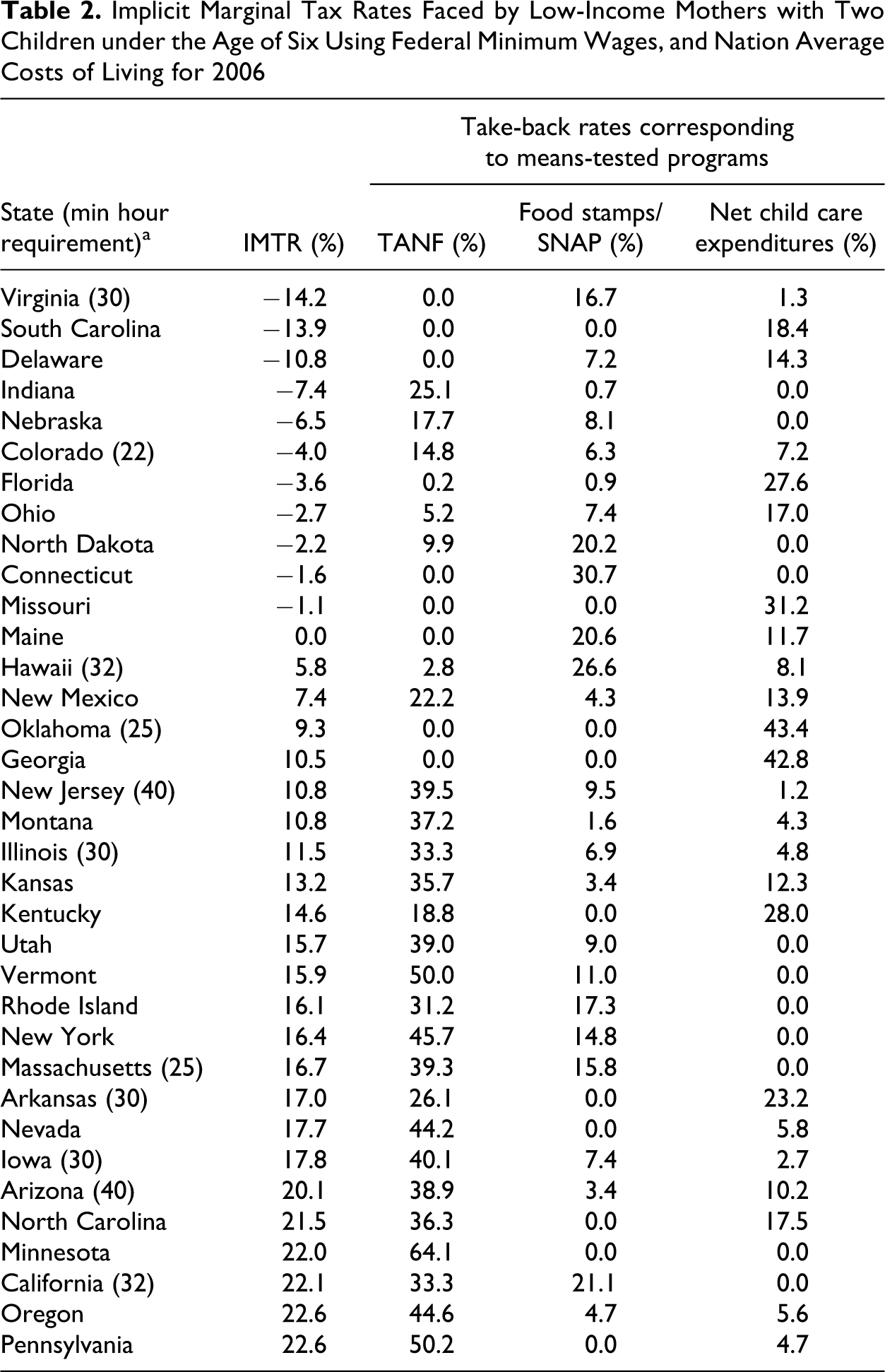
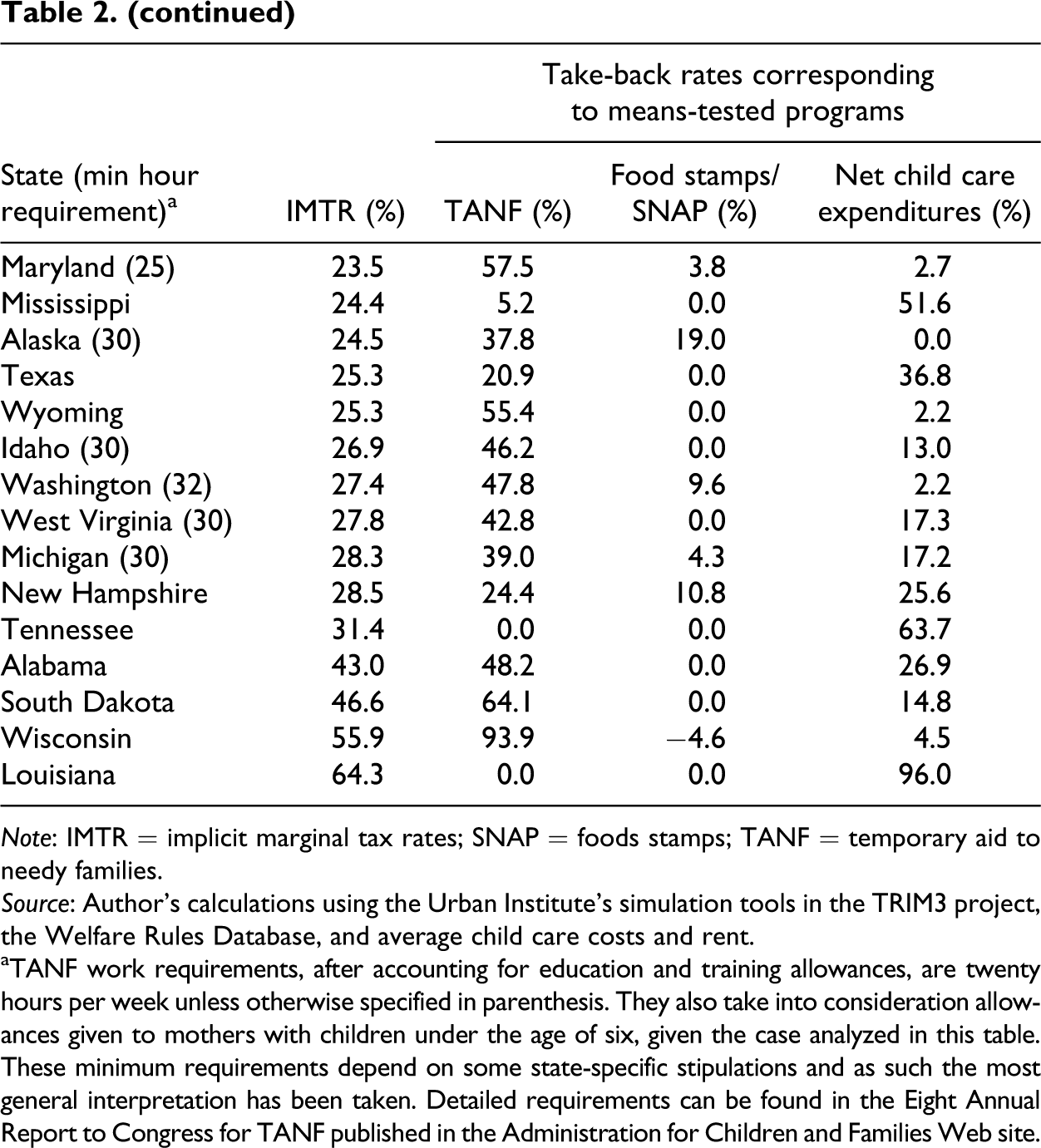
Note: IMTR = implicit marginal tax rates; SNAP = foods stamps; TANF = temporary aid to needy families.

Source: Author’s calculations using the Urban Institute’s simulation tools in the TRIM3 project, the Welfare Rules Database, and average child care costs and rent.

^aTANF work requirements, after accounting for education and training allowances, are twenty hours per week unless otherwise specified in parenthesis. They also take into consideration allowances given to mothers with children under the age of six, given the case analyzed in this table. These minimum requirements depend on some state-specific stipulations and as such the most general interpretation has been taken. Detailed requirements can be found in the Eight Annual Report to Congress for TANF published in the Administration for Children and Families Web site.

Table 3.

Implicit Marginal Tax Rates Faced by Low-Income Mothers with Two Children under the age of Six Using State Minimum Wages, and State Costs of Living for 2006

		Take-back rates corresponding to means-tested programs
State (min hour requirement)^a	IMTR (%)	TANF (%)	Food stamps/SNAP (%)	Net child care expenditures (%)
Tennessee	−32.3	0.0	0.0	0.0
South Carolina	−27.6	0.0	4.9	0.0
Mississippi	−22.6	5.2	0.0	4.5
Georgia	−22.6	0.0	0.0	9.6
Texas	−13.0	0.0	0.0	19.3
Missouri	−13.0	10.1	6.3	3.1
Delaware	−10.3	8.5	10.0	3.9
Connecticut	−7.6	0.0	24.8	0.0
Indiana	−7.6	25.1	0.7	0.0
Nebraska	−2.7	17.7	12.1	0.0
Colorado (22)	−1.8	11.2	6.5	12.9
Ohio	−1.6	5.2	9.0	17.0
Arkansas (30)	1.1	28.6	4.9	0.0
Florida	2.0	20.4	2.5	11.6
Kentucky	4.0	31.6	0.0	4.7
Oklahoma (25)	6.5	37.0	1.4	2.3
Hawaii (32)	7.6	15.4	15.6	7.0
North Dakota	8.7	9.9	31.6	0.0
Maine	9.8	6.9	23.1	12.1
New Mexico	9.9	33.2	7.0	2.9
New York	13.4	48.5	9.6	0.0
Kansas	13.7	48.0	4.0	0.0
Montana	13.7	37.2	4.7	4.3
Utah	15.5	39.0	9.0	0.0
Virginia (30)	15.7	0.0	0.6	47.5
Massachusetts (25)	15.7	21.8	11.5	20.1
Rhode Island	16.4	35.6	13.4	0.0
Louisiana	17.3	0.0	0.0	48.9
Nevada	17.7	46.6	0.0	3.4
California (32)	18.7	38.1	12.6	0.0
Vermont	19.1	54.9	7.3	2.1
Iowa (30)	19.7	40.1	12.3	0.0
North Carolina	21.5	36.3	0.0	17.5
Illinois (30)	21.6	33.4	4.4	17.2
Minnesota	21.6	64.3	0.0	0.0
Pennsylvania	22.6	50.2	0.0	4.7
Maryland (25)	23.3	19.4	3.8	40.6
Idaho (30)	23.5	46.2	0.0	9.6
Arizona (40)	25.0	38.9	1.2	17.3
Wyoming	25.4	56.1	0.0	1.7
Alabama	26.0	48.2	0.0	9.6
Alaska (30)	26.5	41.0	17.5	0.0
West Virginia (30)	27.8	52.9	0.0	7.2
Michigan (30)	28.0	26.0	4.3	30.0
New Hampshire	29.4	0.0	8.1	53.6
Washington (32)	30.0	48.7	9.0	1.4
South Dakota	38.8	64.1	7.4	0.0
Oregon	42.2	70.9	0.0	3.9
Wisconsin	48.0	84.9	−2.8	4.1
New Jersey (40)	49.9	28.2	2.9	53.6

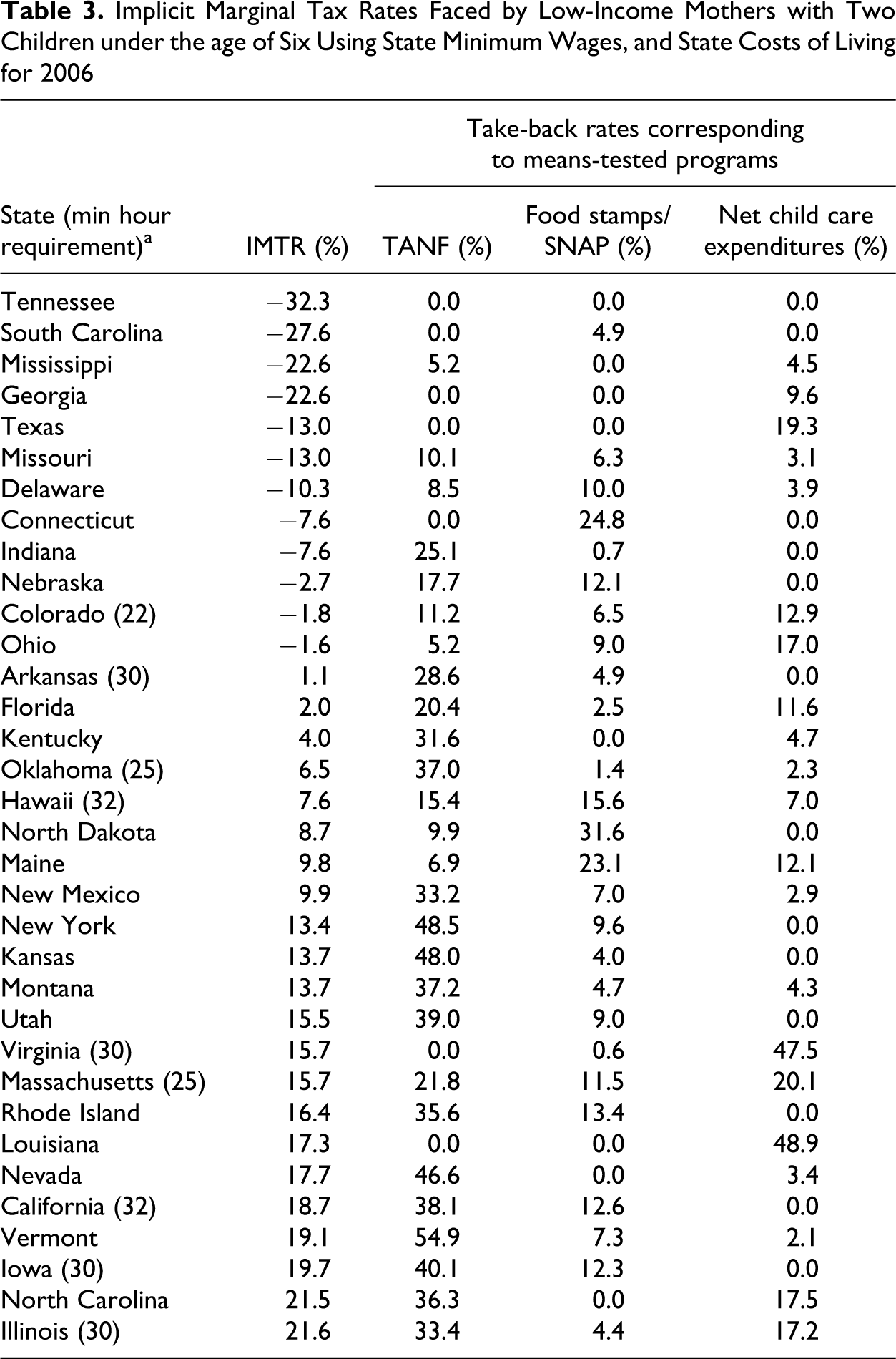
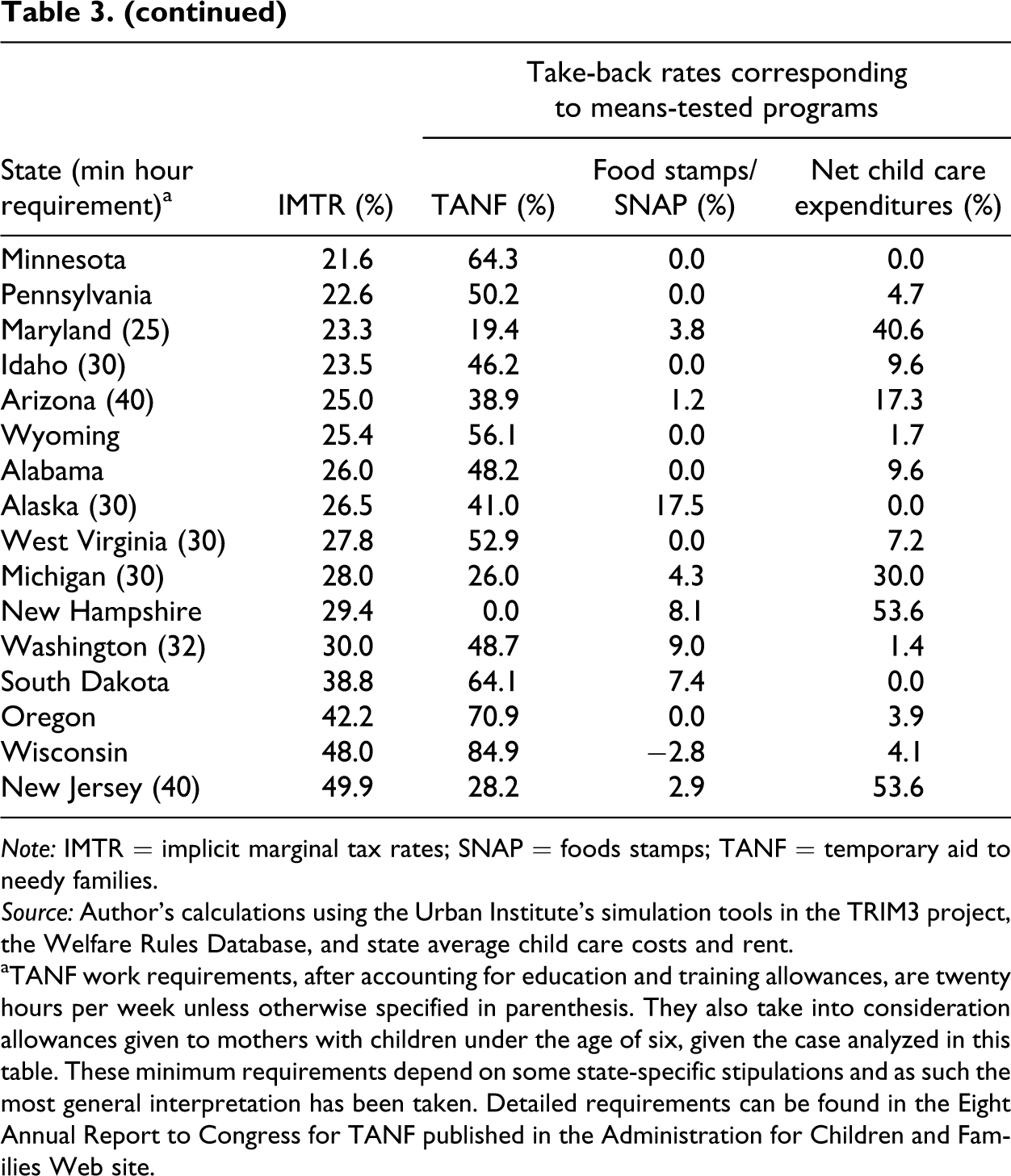
Note: IMTR = implicit marginal tax rates; SNAP = foods stamps; TANF = temporary aid to needy families.

Source: Author's calculations using the Urban Institute’s simulation tools in the TRIM3 project, the Welfare Rules Database, and state average child care costs and rent.

The results displayed in both tables not only allow us to increase awareness among researchers about the importance of states' cost of living when determining the magnitude of IMTRs for low-income mothers but also illustrate that it is hard to identify the driving forces of the magnitude of state MTRs under perfect work compliance. For instance, Table 3 shows that adjusting for wages and the cost of living, Wisconsin and New Jersey have the highest cost to compliance. However, in the case of Wisconsin, this is mostly due to a relatively high TANF benefit and a fast loss of that benefit. New Jersey, on the other hand, has a much more prudent reduction of TANF benefits, but a large increase in out of pocket child care expenses relative to the increase in earning from work. Note also that the compliance rules are different as New Jersey recipients are subject to stricter work requirements. Louisiana and Nevada show a similar pattern, though the overall IMTRs are lower at around 17 percent. As expected, when the calculation of IMTRs uses the state minimum wages (Table 3), those states with higher the federal minimum wage tend to show higher effects from the reduction on TANF benefits. That is the case of Vermont ($7.25), California ($6.75), and Oregon ($7.50). Nonetheless, that does not mean that higher TANF take - back rates are necessarily associated with higher IMTRs. California and Florida ($6.40) experience lower IMTRs despite the change of wage and increase in TANF overall reduction rate. Finally, Connecticut is the only state that appears to be heavily influenced by the phase-out of Food Stamps. However, Connecticut is very generous with its benefits providing high income disregards, which prevent major changes in TANF benefits in this range, as well as with the coverage of child care costs. Both higher wages, which translate into relatively higher gross income, and the program’s generosity in Connecticut prevent the Food Stamps from making considerable allowances for child care.

Analysis of Assumptions Using Selected States

The previous section suggests that changes in the assumptions can yield different and significant changes in the resulting state IMTRs, even when holding state work requirements constant. Consequently, analyzing the role of assumptions deserves a more detailed examination than just looking at the overall reduction rates of welfare benefits. This section examines the effect of certain assumptions for a selected group of states.

Child Care Provision and Work Requirements

Until now, it has been assumed that child care is provided according to the mother’s needs. This means that mothers are allowed to use child care on an hourly base, without having to incur extra costs for hours in which they are not working. Yet, as Tables 2 and 3 show, the resulting IMTRs under full work compliance can be heavily influenced by the change in child care costs, even when calculated linearly. Altering this assumption can yield very different results, making it a determinant of IMTRs that deserves special attention. The linear assumption can be realistic if a mother finds a somewhat informal source of child care such as a family care facility, a nanny, or even an understanding and lenient care facility. However, it is also common to find private care facilities that will only allow for two types of payment: part-time and full-time. Under such conditions, a mother that is working twenty-five hours a week (i.e., (the Maryland requirement) will be forced to pay as if she had her children in care for forty hours a week or more. Evidently, this may create cliff effects equivalent to those documented by Romich, Simmelink, and Holt (2007) for other programs. Note that the resulting changes also depend on the flexibility in work requirements set by the state.

For simplicity and comparability reasons, assume the same two scenarios described above for the state of Florida, Idaho, Iowa, and Wisconsin. Again, using federal averages allow us to make comparisons among states given that it assumes the same costs and wages for all states. In Florida, the work requirement of twenty hours per week assures that there would be no change in child care out of pocket expenses if the compliant mother has to pay hourly or on a full-time/part-time basis. Since the hourly rate is calculated by dividing the total costs by the number of hours, the costs for child care would be the same under the two scenarios.¹¹ However, assume that work requirements were thirty hours per week as it is the case for the other three states. In that case, a mother in Florida would earn approximately $669 per month. The child care cost rate would double to the full-time rate, and out of pocket expenses, net of subsidies, would increase to $465, instead of $123 (for the actual case of twenty-hour requirement). Now, the increase in child care expenses as a percent of additional earned income when the mother transitions quickly into full compliance, is almost 70 percent instead of 28 percent.

As expected, this increase does not occur if the work requirement was thirty hours and the child care received is charged hourly. In that case, the increase in child care as a percent of earned income is 29 percent, slightly above the case of a twenty-hour requirement. The ending result would be an overall increase of the IMTR from −4 percent to 37 percent. Similar but smaller scale results are found when looking at the scenario in which state costs and wages are used. In that case, the change in work requirements would increase the IMTR from 2 percent to approximately 12 percent when cost is computed on a part-time/full-time basis and 10 percent when computed hourly. This is partly due to the higher wage ($6.40), and partly to the lower than average cost of child care ($941 for full-time).

Idaho, Iowa, and Wisconsin have work requirements of thirty hours per week. The Idaho IMTR using federal assumptions for part-time/full-time child care is approximately 68 percent while the one under hourly charge is approximately 26 percent. Using state costs, the overall IMTR goes from 26 percent to 23 percent if charged hourly. Child care costs in Idaho are low ($780) and subsidies are somewhat generous at the higher margins. For instance, even when the care is not charged by the hour, the subsidy leaves the mother with a copayment of $84 per month whether she works thirty, thirty-five, or forty hours per week. On the other hand, since the cost is lower at thirty hours when charged hourly, the generous subsidy leaves her with a copay of $64 per month, meaning very small changes between the two scenarios. Interestingly, even though Iowa also experiences a decrease in IMTR when child care is charged hourly at the thirty-hour work requirement, this does not happen if this requirement was twenty hours. Furthermore, contrary to Florida and Idaho, the overall IMTR is lower under the actual requirements compared to if we changed it to twenty hours. This result highlights the importance of program designs in the effort to encourage work. Iowa, like several other states, does not provide any child care subsidies until the work requirement is met. Although seemingly harsh, this incentivizes the mother to meet the requirement so she does not have to bear the full cost of care.

However, lower out of pocket expenses does not mean that the mother will face no marginal taxation, as she is still responsible for a copayment as large as $207 per month when using state costs. In some states the child care subsidies are not provided until the recipient meets all work requirements, including education and/or training activities. Consequently, some mothers may effectively need more care time that the one needed for remunerated work, and the amount of child care copay must be calculated as if the parent were working more hours. This has implications for the overall MTR given that the effective take - back rate for child care subsidy is taken as percentage of a lower change in earnings.¹² Wisconsin, on the other hand, covers most of the cost of child care and its high MTR stems from other sources (e.g., TANF).

Assuming that states rules are adjusted to wages and costs of living, I focus on the results from Table 3 hereafter. This allows me to compare the effect that a simple change in only one parameter may have in the amount of benefits received and thus the IMTR when everything else remains equal (including the work requirement for each state).

Minimum Wages

Given the nature of these programs, an increase in wages will necessarily affect the amount of benefits received. This is true for all benefit programs, including the EITC. However, as noted above, the rate of increase in EITC benefits and tax liabilities does not change within this income range, so these programs will not affect the overall IMTR. However, because of TANF income disregards, we may observe that when everything else is held constant, higher minimum wages will change the relative ratio of changes in TANF benefits to changes in earnings. This change is not uniform nor equally predictable for all states, as the BRR also plays a role once the mother has topped the income disregard. Florida, Wisconsin, and Oregon are interesting cases worth detailing. All had minimum wages above the federal minimum wage for 2006, but had also completely different TANF designs. In Florida, for instance, when a mother faces state costs but works at the federal minimum wage ($5.15), her income is disregarded up approximately twenty working hours per week. After that, her benefits start being reduced, albeit not at a constant rate since benefits are affected by the expense of child care. In Wisconsin, regardless of the assumptions, the mother is initially eligible for $628 per month but loses all of it as soon as she starts working. This translates into a very steep implicit TANF BRR, which is only affected by increases in wages in that such increases change the relative decrease of the TANF benefit. Indeed, the TANF take-back rate decreases from 94 percent to 85 percent when comparing scenarios under federal minimum wage and state minimum wage. Instead, given the work requirements in Florida and Oregon, the TANF take-back rate increases with wages, increasing the overall IMTR. In fact, the TANF take-back rate increases by as much as twenty percentage points in Oregon ($7.50), from 50 percent to approximately 71 percent.

These examples confirm that changes in some assumptions can create diverse changes within and across states. Moreover, they suggest that the changes are complicated and not at all predictable, adding to the complexity of IMTR calculations for the purpose of explaining economic behaviors of uneducated low-income mothers.

Rent, Child Care Costs, and Age of Children

Generally, changes in rent values generate rather small changes in the IMTRs considered here. This result will differ significantly if the mother also receives housing subsidies. To the extent that it is not included here, the rent value will only affect the Food Stamps benefit. The change will likely be minimal given the small variation of median rent values across the nation. An important fact to highlight by looking Louisiana, Maine, California, and New Hampshire is that an increase in rent will likely decrease the overall IMTR a few percentage points. This is due to a flattening effect in the Food Stamps BRR.

Similarly, changes in child care cost will cause changes in the overall IMTR. The preceding analysis of child care provision is a somewhat more complicated than is the one in which the only thing that changes is the cost. However, it lets us infer what we can find if indeed we shifted the costs of care when all other assumptions remain the same: overall IMTRs increase with child care costs. This increase is not linear and hard to predict without the actual calculation. In Kentucky, where the work requirement is twenty hours per week, the part-time child care cost is $427, well below the national average of $532. If the mother of two children were to pay at the nation’s average, she would be responsible for $125 copayment. At the state cost, this same mother is only responsible $21 per month. This translates into an effective IMTR close to 4 percent, as opposed to 14 percent had she had to pay the national average. New Jersey, on the other hand, has a well above average child care cost. A similar comparison reveals that by paying state rates the complying mother faces an IMTR of almost 50 percent, compared to 21 percent if paying the nation’s average for the full-time cost.¹³

The age of children is perhaps one of the most overlooked, yet very important, factors determining the MTRs of low-income single mothers. All of the analysis presented in this article thus far assumes that the single mother has two children under the age of six. However, as stated under the description of TANF, mothers may still qualify if children are younger than eighteen. Changing this assumption has two effects in many states. First, hypothetically, older kids can attend school and child care and child care subsidies are no longer needed. Second, in many states, the work requirement is different for those with older children. Most states actually require thirty hours of work per week, but many allow for a reduction if children are below younger than six. As a result, a mother with two children over six faces a different requirement than a mother with children just under the age of six.

I illustrate the effect of this assumption by analyzing the case of North Carolina. For simplicity, I assume that either both children are older than six or both are younger than six. Table 4 displays the computed benefits for both scenarios. North Carolina mandates that mothers with children six or older should work thirty-five hours. However, the rules also say that these mothers are allowed to use fifteen of those hours in job training/educational activities. The mother then is allowed to choose between effectively working twenty or thirty-five hours, whichever is more lucrative. The mother of the younger children is allowed to work only twenty hours. In North Carolina, at the given minimum wage, child care subsidies are not provided until the mother works more than twenty-five hours a week. Thus, she has an incentive to engage in some job related activity that allows her to obtain the subsidy. If this is the case, she may be able to obtain a subsidy large enough that leaves her with an expense of approximately $78. This may seem small to some, but as a percentage of additional earned income it accounts for almost 17 percent, translating into an implicit MTR of 21 percent.

Table 4.

Net Disposable Income for a North Carolina Single Mother with Two Children of Different Ages for 2006

	Hours per week worked
	Younger children		Children over six
	No work	Twenty hours	No work	Twenty hours
Category	No work	Twenty hours	No work	Twenty hours
Earnings	0	446	0	446
Federal and state income tax	0	0	0	0
EITC	0	178	0	178
Payroll tax	0	−34	0	−34
TANF	272	110	272	110
Food Stamps	395	395	395	395
Child Care Expense	0	−78	0	0
Net Income	$667	$1,017	$667	$1,095
IMTR		21.5%		4.0%

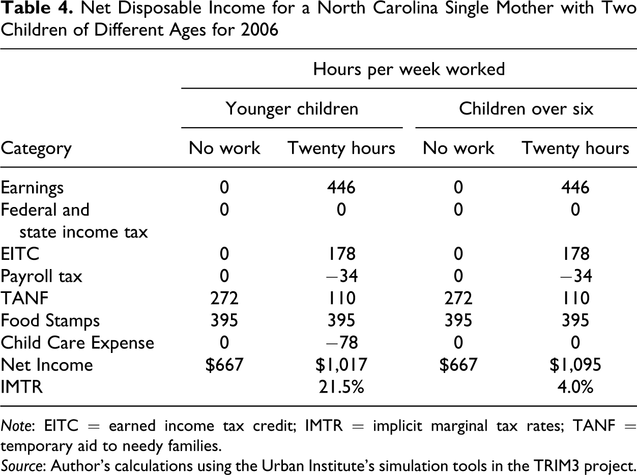
Note: EITC = earned income tax credit; IMTR = implicit marginal tax rates; TANF = temporary aid to needy families.

Source: Author’s calculations using the Urban Institute’s simulation tools in the TRIM3 project.

The mother with older will face an effective IMTR close to 4 percent if she only works for wages up to twenty hours, and 6.5 percent if remunerated work amounts to thirty-five hours (not shown). As evidenced, the rules on ages and work requirements can also translate into significant changes in the resulting simulation. Moreover, the understanding of these rules can be lengthy and cumbersome for both the researcher and the recipient. Like in the previous cases, this example illustrates the complexity of the interactions among programs and hence the calculation of implicit MTRs, even when assumptions attempt to replicate the most realistic scenario.

Marital Status

The welfare reform also stipulated its intention to stimulate marriage, given the increased percentage of single mothers in the welfare rolls. Although not the main concern of this article, it is pertinent to briefly discuss the implicit marginal effect of marriage for a single mother compliant with the state working rules. A similar calculation was done by Alm, Dickert-Conlin, and Whittington (1999) to calculate the marriage penalty for a Pennsylvania mother that does not work, and marries the father of her children. A quick back-of-the-envelope calculation suggests that when the complying mother marries the father who has been working forty hours a week at the state minimum wage, they not only lose TANF and FS benefits ($170 and $395), but also incur $43 in additional child care expense. This offsets the gain in reduced tax liabilities and increase in EITC (total of $292) resulting in a marriage penalty of ($328 per month).

Conclusion

In this article I estimate the IMTR for all fifty states under a variety of assumptions. Constructing accurate IMTR estimates can be extremely cumbersome. Every state has different program eligibility rules, phase-out patterns, and work requirements. I find that the estimated rates vary significantly when regional differences, such as prevailing minimum wage and child care costs, are taken into account.

These estimates are very sensitive to the construction of the hypothetical household and program participation rates. Changes in assumptions, location, and work requirements produce estimates that vary significantly and, perhaps more troubling, unpredictably. Analysis which relies on estimates of IMTRs facing low-income households must be done with care given the large influence relatively minor assumptions can have. Researchers and policy makers interested in labor supply at the intensive margins should be wary of the incentives provided to those that want to comply with the work requirements specified. These are especially important when estimating the implicit MTRs for low-income families and can heavily influence the work compliance rates, a source of increasing (or decreasing) funding to states from the federal government.

Footnotes

Acknowledgments

The author wants to thank Russell Sobel, Tami Gurly-Calvez, George Hammond, Christopher Coyne, and Donald Lacombe for helpful comments. Additionally, the author is indebted to the editor of Public Finance Review, James Alm, and two anonymous referees for valuable input on the article. Information presented here is derived in part from the Transfer Income Model, Version 3 (TRIM3) and associated databases. TRIM3 requires users to input assumptions and/or interpretations about economic behavior and the rules governing federal programs. Therefore, the conclusions and/or errors presented here are attributable only to the author of this manuscript.

The author declared no potential conflicts of interest with respect to the research, authorship, and/or publication of this article.

The author received no financial support for the research, authorship, and/or publication of this article.

Notes

References

Acs

Gregory

Coe

Norma B.

Watson

Keith

Lerman

Robert I.

. 1998. Does Work Pay? An Analysis of the Work Incentives under TANF. Washington, DC: The Urban Institute.

Alm

James

Dickert-Conlin

Stacy

Whittington

Leslie A.

. 1999. “Policy Watch, The Marriage Penalty.” Journal of Economic Perspectives 13:193–204.

Ellwood

David T.

Liebman

Jeffrey B.

. 2001. “The Middle Class Parent Penalty: Child Benefits in the U.S. Tax Code.” National Bureau of Economic Research Working Paper No. 8031, Cambridge, MA.

Gallagher

Jerome

Gallagher

Megan

Perese

Kevin

Schreiber

Susan

Watson

Keith

. 1998. Temporary Assistance for Needy Families (TANF) One Year after Federal Welfare Reform: A Description of State TANF Decisions as of October 1997. Washington, DC: The Urban Insitute.

Garfinkel

Irwin

Orr

Larry L.

. 1974. “Welfare Policy and The Employment Rate of AFDC Mothers.” National Tax Journal 27:275–84.

Holt

Stephen D.

Romich

Jennifer L.

. 2007. “Marginal Tax Rates Facing Low-and-Moderate-Income Workers Who Participate in Means-Tested Transfer Programs.” National Tax Journal 50:253–76.

Keane

Michael

Moffitt

Robert

. 1998. “A Structural Model of Multiple Welfare Program Participation and Labor Supply.” International Economic Review 39:553–89.

Koester

Reinhard B.

Kormendi

Roger C.

. 1989. “Taxation, Aggregate Activity and Economic Growth: Cross-Country Evidence on Some Supply-Side Hypotheses.” Economic Inquiry 27:367–86.

Lugalla

Terry A.

2005. Participation of Mothers in Government Assistance Programs: 2001. Washington, DC: Technical Report, Household Economic Studies, US Census Bureau.

10.

Meyer

Bruce D.

2002. “Labor Supply at the Extensive and Intensive Margins: The EITC, Welfare, and Hours Worked.” American Economic Review 92:373–9.

11.

Meyer

Bruce D.

, 2010. “The Effects of the Earned Income Tax Credit and Recent Reforms.” In Tax Policy and the Economy. 24: 153–180. Chicago and London: University of Chicago Press; Cambridge, Mass.: National Bureau of Economic Research.

12.

Meyer

Bruce D.

Rosenbaum

Dan T.

. 2000. “Making Single Mothers Work: Recent Changes in Tax and Welfare Policy and their Effects.” National Tax Journal 53:1027–62.

13.

Meyer

Bruce D.

Rosenbaum

Dan T.

. 2001. “Welfare, the Earned Income Tax Credit, and the Labor Supply of Single Mothers.” Quarterly Journal of Economics 116:1063–114.

14.

Meyer

Bruce D.

Sullivan

James X.

. 2004. “The Effects of Welfare and Tax Reform: The Material Well-Being of Single Mothers in the 1980s and 1990s.” Journal of Public Economics 88:1387–420.

15.

Moffitt

Robert A.

2003. “The Temporary Assistance for Needy Families Program.” In Means-tested transfer programs in the United States, 291–363. NBER Conference Report series.

16.

Reed

W. Robert

Rogers

Cynthia L.

Skidmore

Mark

. 2011. “On Estimating Marginal Tax Rates for U.S. States.” National Tax Journal 64:59–84.

17.

Romich

Jennifer L.

2006. “Difficult Calculations: Low–Income Workers and Marginal Tax Rates.” Social Service Review 80:27–66.

18.

Romich

Jennifer L.

Simmelink

Jennifer

Holt

Stephen D.

. 2007. “When Working Harder Does Not Pay: Low-Income Working Families, Tax Liabilities, and Benefit Reductions.” Families in Society 88:418–26.

19.

Sammartino

Frank

Toder

Eric

Maag

Elaine

. 2002. “Providing Federal Assistance for Low-Income Families through the Tax System: A Primer.” Washington, DC: Technical Report, The Urban Institute.

20.

Shaviro

Daniel N.

1999. Effective Marginal Tax Rates on Low-Income Households. Washington, DC: Technical Report, Employment Policies Institute.

21.

Williams

Robert G.

1975. Public Assistance and Work Effort: The Labor Supply of Low-Income Female Heads of Household. Research Report Series No. 119. Princeton, NJ: Princeton University.

22.

Wilson

Paul

Cline

Robert

. 1994. “State Welfare Reform: Integrating Tax Credits and Income Transfers.” National Tax Journal 47:655–76.

23.

Wolfe

Barbara

. 2002. “Incentives, Challenge, and Dilemmas of TANF: A Case Study.” Journal of Policy Analysis and Management 21:577–86.