The Demand for Municipal Infrastructure Projects

Abstract

Many studies have investigated the determinants of current local public expenditures whereas only a few have studied the factors explaining the capital decision-making process at the local government level. This study uses a panel data set of Connecticut town and cities over the 2000 to 2010 period to estimate the local public demand for various types of capital infrastructure projects. The multiple regression analysis reveals a number of insights regarding the capital-investment decision of local communities. First, unlike the demand for current expenditures, the demand for capital-investment projects is elastic with respect to tax price. Second, unlike the demand for current expenditures, the demand for capital projects is not directly related to changes in income. Finally, intergovernmental grants are shown to be an important determinant of capital investment spending although the specific aid doesn’t always seem to stick where it initially hits.

Keywords

public capital demand for public infrastructure spending intergovernmental aid price and income elasticity

Researchers have long been interested in empirically explaining the economic behavior of local governments. Most of the studies have focused on the determinants of current local public expenditures on services such as education, highways, parks, and libraries (evolving from Borcherding and Deacon [1972] and Bergstrom and Goodman [1973] to, much more recently, Bates and Santerre [2013]). Findings from these empirical studies have offered numerous insights into municipal behavior including elasticity estimates of the demand for local public services with respect to tax price, income, and intergovernmental aid. Elasticity estimates such as those have been important when formulating local public policies.

Few studies, however, have investigated the main drivers influencing investment spending on collectively financed local capital infrastructure projects. This neglect is somewhat surprising given the relatively large amount of infrastructure spending that takes place at the local level in the United States. According to the Statistical Abstract of the United States (2012), capital spending by local governments amounted to $236 billion or 15 percent of current expenditures for the fiscal year ending 2008. In addition, many policy makers believe municipal investment on infrastructure should be much greater than this 15 percent figure because of the sizable benefits from capital projects. For example, studies by the US Conference of Mayors (2008) and the US Department of the Treasury (2012) cite large productivity gains from public infrastructure investments based on research such as Aschauer (1989) and Munnell (1990, 1992). Also, the benefits of public infrastructure investment spending may spill into the private sector. As one example, road improvements may improve the efficiency of transporting goods to the private marketplace. As another example, Haughwout (1997) shows empirically that housing values appreciate in response to local public infrastructure investment spending.

Holtz-Eakin (1991), Holtz-Eakin and Rosen (1989, 1993), Temple (1994), and Balsdon, Brunner, and Rueben (2003) are among the more ambitious studies investigating the determinants of public infrastructure investment spending at the subnational levels of government. While these studies have shed considerable light on the capital investment decision-making process by government, they are deficient in several important respects. First, some of these studies have combined state and local investment spending. But factors affecting state investment behavior may not similarly impact local government behavior. Second, these previous studies lacked information on the number and various types of individual capital projects (e.g., highway, building, waste facilities, etc.) and, as a result, focused entirely on the determinants of total infrastructure investment spending. It stands to reason that some important information may have been lost by focusing entirely on total investment spending rather than its individual components.¹ Finally, all of these previous studies have been cross-sectional in nature. As a result, these studies may have missed out on the dynamic aspect of capital infrastructure investment spending. In addition, unobservable heterogeneity may have produced biased estimates because of the cross-sectional approach taken in these earlier studies.

This article extends previous research on this topic by using a panel data set of Connecticut towns and cities to estimate the local demand for capital infrastructure projects. Based upon data from the Local Capital Improvement Program (LoCIP) in Connecticut, we are able to identify the number and different types of projects that each community undertook during each year from 2000 to 2010. Based upon a median-voter model of local government investment-decision making, we empirically investigate the various factors influencing the demand for these different projects. Because a panel data set is used, we are able to control for time- and community-fixed effects.

The empirical results yield a number of important insights into the local government capital decision-making process. First, unlike the demand for current expenditures, the demand for capital-investment projects is elastic with respect to tax price. Second, unlike the demand for current expenditures, the demand for capital projects is not directly related to changes in income. Finally, intergovernmental grants are shown to be an important determinant of capital investment spending although the specific aid doesn’t always stick where it initially hits.

The following section provides the conceptual model behind the empirical framework and clarifies the specific data, variables, and empirical specification used in the analysis. The third section reports and discusses the empirical findings whereas the last section of this article offers a summary and some concluding remarks.

Empirical Model of the Demand for Local Public Infrastructure Projects

Conceptual Model of the Median Voter

Numerous researchers, beginning with Borcherding and Deacon (1972) and Bergstrom and Goodman (1973), have found that a median-voter model represents a useful way of depicting how local communities make decisions. Based upon various assumptions such as single-peaked preferences, public choice theory predicts that the median demand dominates over all other demands when decisions are driven by a simple-majority rule within a direct democratic setting (Bowen 1943).² Moreover, the median demand may dominate in a representative democracy if politicians gravitate toward the middle of the preference distribution to maximize their number of votes (Downs 1957). We, thus, begin by supposing that local public decision makers maximize the utility of the median voter, whose utility function is assumed to depend on three goods and to take the following general form:

U = U (K, G, X) .

In equation (1), K stands for the current stock of local public capital infrastructure, G represents the amount of current local public goods (i.e., from current spending), and X represents the amount of private goods. The amount of K at each point in time is dependent upon the previous stock of capital, $\overset{ˉ}{K}$ its rate of depreciation, d, and any new public capital investment, I, such that $K = (1 - d) \overset{ˉ}{K} + I$ . The utility function of the median voter is maximized by local public decision makers subject to this budget constraint:

Y + s A = s_{1} I + s P_{G} G + P_{X} X .

The two variables to the left of the equality sign represent the median-voter’s yearly income, Y, and share, s, of various types of intergovernmental aid, A. These funds are assumed to be exhausted by expenditures on new capital projects and current public and private goods with s ₁ and sP_G , standing for the median-voter’s tax prices for local municipal investment and local public goods, respectively, and P_X reflecting the price for the private good. Given that local public goods are generally financed through the property tax system, the median-voter’s tax share, s, can be determined by dividing the value of his home, V, by the total market value of all assessed properties in the community or V/V_T . The tax price for local public investment is specified in the following manner with r representing the market interest rate for municipal debt:

s_{I} = s (1 + r) .

The market interest rate, in turn, is assumed to be an increasing function of the amount of outstanding municipal debt, D, owed by the community, or r = r(D). Given that greater transaction costs are typically associated with external borrowing, note that r may be lower than the market rate if internal funds are used to finance the municipal capital projects.

Conceptually, it follows from this maximization process that the median-voter’s optimal amount of local public capital-investment projects, or capital-investment spending, can be written as a function of the various parameters of the model, or:

I = I (d, \overset{ˉ}{K}, s, Y, s A, P_{G}, P_{X}, D) .

Notice that equation (4) captures the three different ways in which local public investment spending might be financed; namely: internal funds through s, intergovernmental aid in the form of sA, and borrowed external funds as reflected in D. Also note that since tax share, s, is found by dividing the median-voter’s house value by the total value of all properties in a community, the wealth of a community also potentially plays a pivotal role in the empirical analysis.

The LoCIP Data and Variables

A panel data set of Connecticut towns and cities over the period from 2000 to 2010 is used to estimate a variant of equation (4) for four different types of local public capital infrastructure projects.³ More specifically, each year, the Connecticut state government distributes $30 million to municipalities for reimbursing the cost of eligible local capital improvement projects, such as road, park, or public building construction activities, under the LoCIP. The share of the $30 million each town receives each year is based on a formula and is added to each municipality’s available LoCIP balance, which results from unspent funds being rolled over from one year to the next. The formula determines each town’s share of the $30 million based on its number of road miles (with a 30 percent weight), population density (25 percent), property wealth per capita (25 percent), and population (20 percent). A municipality can request LoCIP funding by completing an application for project approval and reimbursement. LoCIP projects may include repairs incidental to reconstruction and renovation, but cannot include ordinary repairs and maintenance of a routine, ongoing nature. Once a municipality expends funds for an authorized LoCIP project, it may apply for reimbursement.

These data from the LoCIP are used to estimate the demand for local public capital-investment projects. For each year, data are available for the outstanding LoCIP balance at the beginning of the year, the number of LoCIP-approved projects in each municipality (which can be zero), the type of project (e.g., road, building, and park), and the amount reimbursed by the State.⁴ When these data are combined with other information about the communities, we are able to estimate the demand for the different types of infrastructure projects that a typical municipality annually undertakes.

For estimation purposes, we follow the spirit of the median-voter literature and measure the median-voter’s tax share, s, by dividing the median sales price for a single-family house by the market value of all properties for each community-year observation. The median-voter’s annual income, Y, for each community-year observation is measured by the median household income in each community.

Three different types of intergovernmental aid, A, are specified in the empirical models: the LoCIP aid balance (LA), road aid (RA), and all other aid (OA). Like the LoCIP funds, total state grants for road improvement also averaged $30 million over the last several years. Road grants are distributed to towns based on a formula involving population and miles of improved and unimproved roads. The other aid category, which largely comprises state grants for current local school spending, is based on a formula relating to aggregate property wealth per pupil, among other factors. Since the LoCIP aid, road aid, and all other aid are based on formulas that do not depend on matching local funds, the various types of aid can be treated as being exogenous for empirical purposes.⁵

The total amount of each type of aid is multiplied by the median-voter’s tax share, s, and reflects how much money the median voter would have received if that particular type of intergovernmental aid was distributed back to taxpayers based upon their relative tax contributions. Notice that the LoCIP “balance” at the beginning of the year is specified as one measure of intergovernmental aid. As such, it reflects a stock rather than a flow measure of intergovernmental aid because communities are allowed to build up the balance over time and expend the funds when it is considered optimal. Given the fungibility of money, the funds in a community’s LoCIP account and the other aid categories could actually be used to substitute or complement for internal funds.

The variables, d, $\overset{ˉ}{K}$ , P_G , and P_X , cannot be specified in the empirical model because data are unavailable for them. However, the inability to specify these specific variables should have little impact on the empirical findings since the multiple regression analysis captures “within rather than between variations” because of the community-fixed effects that are specified in the estimation equations. That is, the variable d likely does not vary much over time within any one community, and to the extent that I alters $\overset{ˉ}{K}$ , over time, some unwanted serial correlation might be introduced if it was actually specified. In addition, since Connecticut is a relatively small state geographically, both P_G and P_X are likely to be similar across communities at a point in time and also change similarly over time so their exclusion from the estimation equation should have minimal, if any, effect on the empirical results.

To remain consistent with the three measures of intergovernmental aid, indebtedness, D, is calculated by multiplying the total amount of long-term debt that a community owes by the median-voter’s tax share. This variable reflects how much money the median-voter would have to pay if all of the borrowed public funds in the past were immediately paid off. Some other covariates are also specified in the empirical model because the median-voter’s utility function may change over time in response to these variables. Specifically, we specify the population (POP) in the community along with the percentage of the population that is elderly (OLD), white (WHITE), and enrolled in local public schools (PUPILS), as well as the unemployment rate (U) for each community-year observation. Population seems an important variable to include in the empirical specification as previous research, such as Ferris and Graddy (1994, 1998) and Brasington (1999), suggests that population size may affect whether communities produce services internally or contract out for services, or consolidate services with other communities. Whether they contract out or consolidate may influence the amount of local public investment spending that takes place within a specific community.

Two different sets of dependent variables are used as measures of I in equation (4) because the amount of money that each community actually spends on the different types of capital construction projects remains unknown. First, we specify the total number of public projects as well as the number of road, building, and park capital infrastructure projects that are undertaken each year in each community as the independent variables in four different equations.⁶ This “number” of projects should provide a quantity or frequency measure of how many capital projects take place each year across and within communities. One problem with this measure of I, however, is that the factors affecting many small projects may be different from those influencing a few large ones. For example, consider two communities. Community A undertakes ten very small projects in a given year while community B undertakes one very large project. In the analysis, we are assuming that the demand for infrastructure is ten times higher in community A than in community B even though community B might be spending more on infrastructure investment than community A.

Thus, as an alternative but potentially complementary measure of I, we also specify how much the state government annually reimbursed for the four different types of projects under the LoCIP. If the annual reimbursement amounts hold some proportionality to the total amount actually expended, then this measure of I should provide an indication of the “willingness to pay” for, rather than the quantity of, capital infrastructure projects.

Specification of the Estimation Equations

All of the equations are estimated in the following logarithmic form using the ordinary least squares procedure for panel data:⁷

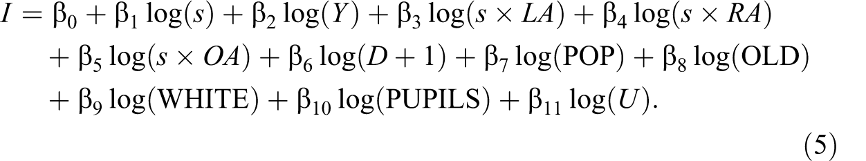
\begin{aligned} I \end{aligned} = β_{0} + β_{1} log (s) + β_{2} log (Y) + β_{3} log (s \times L A) + β_{4} log (s \times R A) + β_{5} log (s \times O A) + β_{6} log (D + 1) + β_{7} log (P O P) + β_{8} log (O L D) + β_{9} log (W H I T E) + β_{10} log (P U P I L S) + β_{11} log (U) .

Notice in equation (5) that the dependent variable is not transformed into its log value because it sometimes takes on the value of zero.⁸ Also notice that $1 is added to the amount of outstanding debt owed by the median-voter, so its log value can be taken for the five community-year observations with no debt.⁹

Because we know only the year when the LoCIP money was paid out and not the year when the projects had been initially planned or demanded, we had to experiment with the data to determine the proper time lag. In particular, the project may have been conceptualized and approved several years before the reimbursement was actually paid out by the state government to the community. Experimentation shows the best fit, in terms of the strength of the statistical relationship between the available LoCIP balance and number of projects, occurs with a two-year lag. The two-year lag seems to work best not only for all infrastructure projects in general but also individually for the different types of projects such as road, building, and park construction.¹⁰

As mentioned previously, community- and time-fixed effects are also specified in the estimated equations to control for baseline unobservable heterogeneity and changes over time that uniformly affect all communities such as the cost of living or new technologies. Also, standard errors are made fully robust against arbitrary heteroscedasticity and serial correlation by clustering them at the community level (Wooldridge 2002).

Empirical Results

Descriptive statistics and the data sources for all of the variables are shown in table 1. For the entire period from 2000 through 2010, 4,429 LoCIP-approved projects occurred in the 169 Connecticut towns and cities (total figures are not shown in table 1). The State reimbursed approximately $610 million for those various projects. As table 1 shows, most of the construction projects involved road improvements following closely by buildings as indicated by both the number of projects and amount of state reimbursements.

Table 1.

Descriptive Variables and Data Sources.

Variable	Mean	Standard deviation	Minimum value	Maximum value	Source of data
List of dependent variables
Total number of projects	2.202	4.98	0	53	1
Road projects	0.821	1.73	0	31	1
Building projects	0.692	2.39	0	31	1
Park projects	0.295	1.69	0	32	1
LoCIP reimbursement for all projects ($)	314,610	1,286,984	0	28,483,484	1
LoCIP reimbursement for road projects ($)	153,735	637,743	0	10,922,324	1
LoCIP reimbursement for building projects ($)	90,932	735,215	0	22,508,201	1
LoCIP reimbursement for park projects ($)	27,641	252,331	0	6,667,587	1
List of independent variables
Population	20,755	24,633	721	144,355	2
Tax share	0.000252	0.000269	.0000163	0.002067	2
Median household income ($)	74,180	23,612	26,055	190,636	2
Fraction white	0.904	0.109	0.130	0.997	2
Fraction old	0.136	0.034	0.028	0.434	2
Fraction pupils	0.165	0.027	0.073	0.257	3
Unemployment rate (%)	5.087	1.95	1.99	16.12	2
Median share of outstanding debt ($)	3,262	2,801.57	0	23,330	3
Median share of available LoCIP funds ($)	35.73	28.53	0.001	180.16	1
Median share of road aid ($)	24.93	20.47	3.53	151.83	4
Median share of other aid ($)	1,353.31	1,175.93	63.05	23,665.46	3

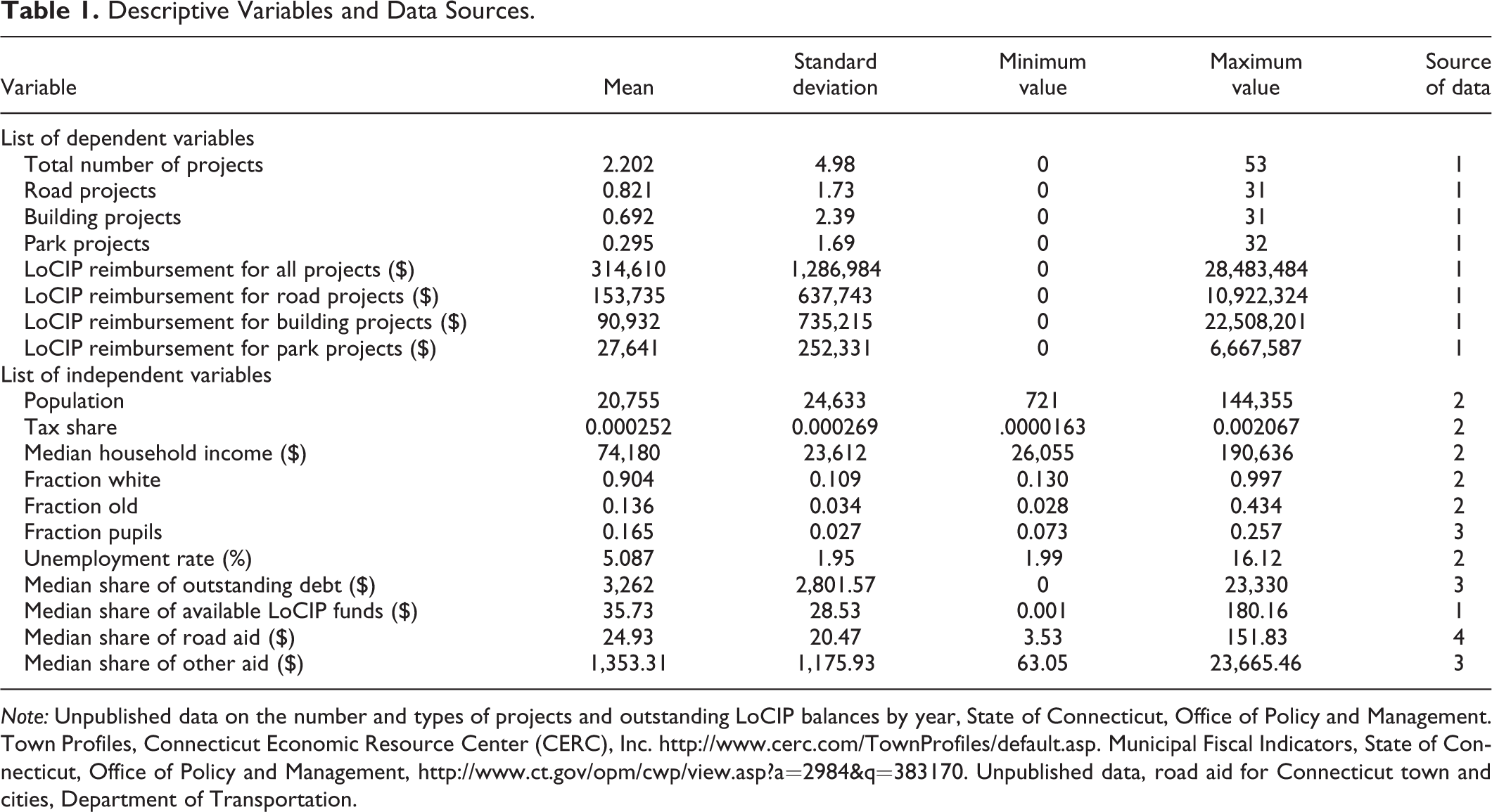
Note: Unpublished data on the number and types of projects and outstanding LoCIP balances by year, State of Connecticut, Office of Policy and Management. Town Profiles, Connecticut Economic Resource Center (CERC), Inc. http://www.cerc.com/TownProfiles/default.asp. Municipal Fiscal Indicators, State of Connecticut, Office of Policy and Management, http://www.ct.gov/opm/cwp/view.asp?a=2984&q=383170. Unpublished data, road aid for Connecticut town and cities, Department of Transportation.

The data in figures 1 and 2 show the trend in the number of LoCIP-approved projects and state reimbursement amounts each year from 2000 to 2010 for all of the towns and cities in Connecticut combined. Trends are shown for some of the individual construction projects as well as for all of the projects collectively. In 2000, 549 construction projects took place throughout the various Connecticut towns and cities. The state reimbursement amount was slightly over $70 million in 2000. Just three years later, those same figures had precipitously slipped to 207 projects and $23 million of reimbursement. By 2006, however, both the number of LoCIP-approved projects and state reimbursement amount had nearly returned to the heights achieved in 2000, only to then fall continuously again over the next three years. A small uptick in the number of projects and state reimbursement amount can be observed from 2009 to 2010. Notice in the figures that the individual projects tend to follow the same general trends as the total figures over time. These data suggest that municipal infrastructure investment changed considerably over the 2000 to 2010 period in Connecticut. It will be interesting to see if our model, as reflected in equation (5), is capable of explaining some of this variation in capital infrastructure development across Connecticut towns and cities over time.

Figure 1.

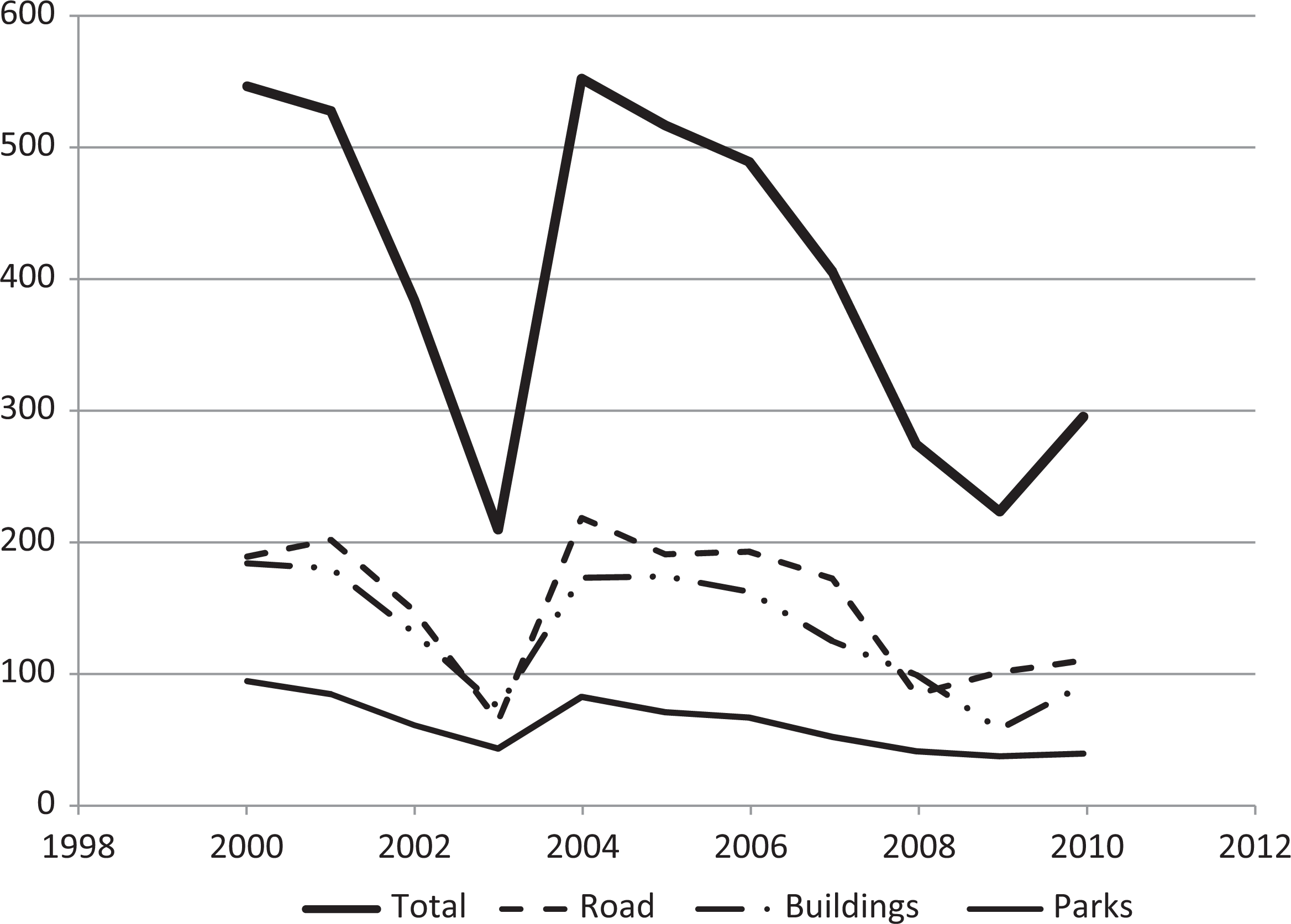
Number of different types of LoCIP-approved public infrastructure projects in Connecticut.

Figure 2.

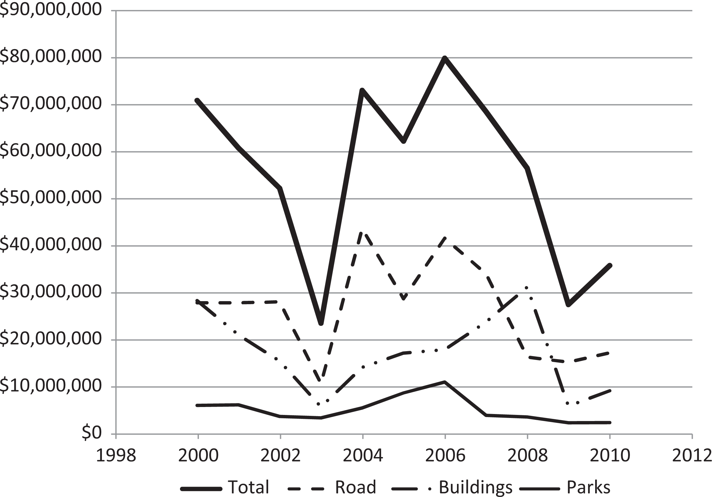
State reimbursement for various types of LoCIP-approved public infrastructure projects in Connecticut towns and cites.

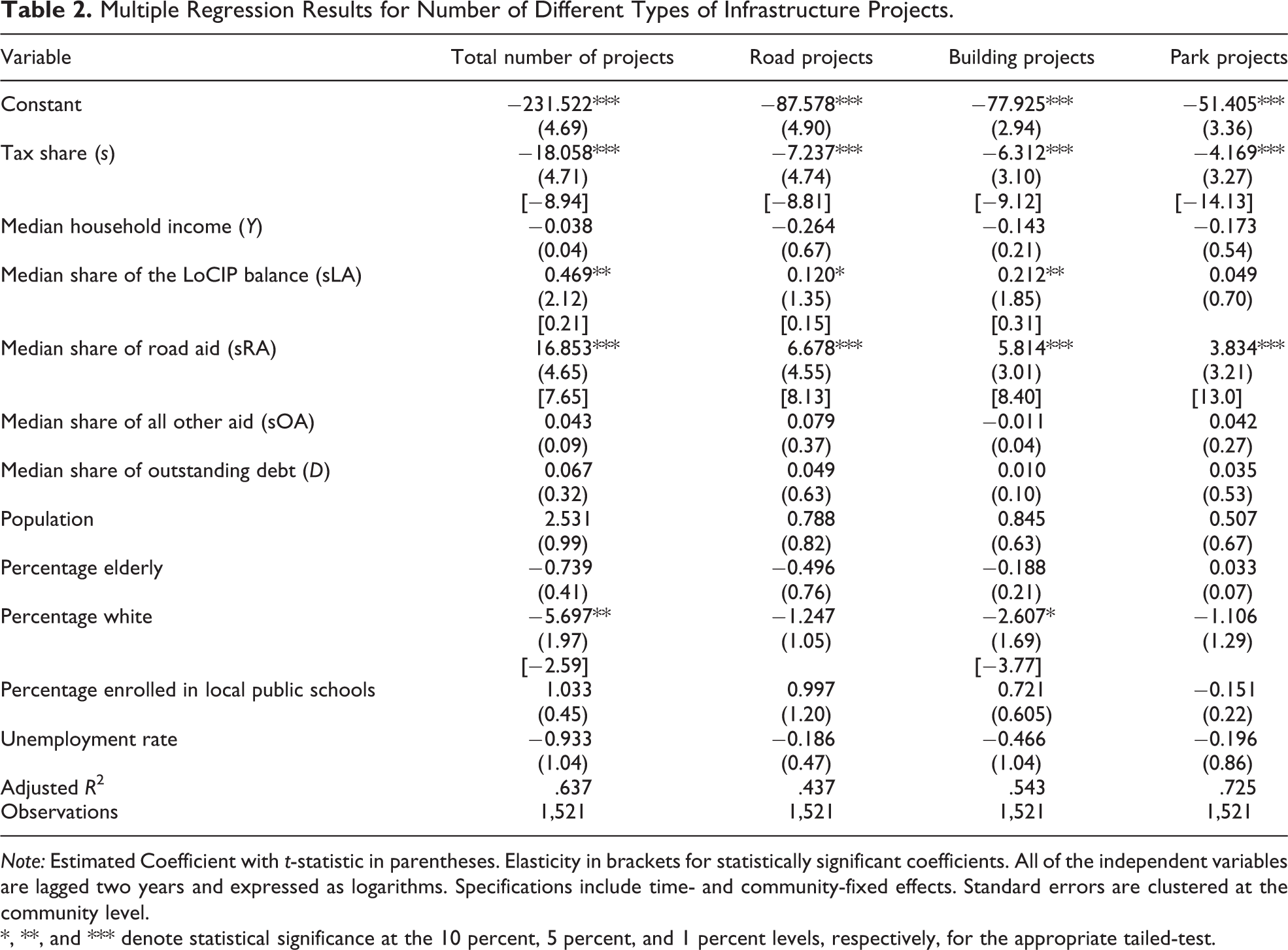
The multiple regression results associated with the number of the various infrastructure projects per year are shown in table 2. The results yield a number of valuable insights about the local public investment decision process. First, notice the consistently negative sign on the median-voter’s tax share in all of the estimated equations, suggesting that the number of capital infrastructure projects is inversely related to the share of investment funds financed internally. This finding may agree with Pagano (2002) who argues that capital spending grows during a boom because more internal funds become available. Moreover, all of the estimated coefficients on tax share are different from zero at conventional levels of statistical significance. Calculated elasticities (shown in brackets) indicate that the overall demand and individual demands for road, building, and park projects are elastic with respect to tax share. Of the three individual types, the demand for public park projects comes across as being the most elastic with respect to tax share. In fact, its estimated coefficient of −14.13 suggests that a 10 percent decrease in the median-voter’s tax share leads to 140 percent more parks projects, ceteris paribus. While this percentage change may appear unreasonably large at first blush, it should be pointed out that the average number of public parks equals only 0.295 for the sample.

Table 2.

Multiple Regression Results for Number of Different Types of Infrastructure Projects.

Variable	Total number of projects	Road projects	Building projects	Park projects
Constant	−231.522*** (4.69)	−87.578*** (4.90)	−77.925*** (2.94)	−51.405*** (3.36)
Tax share (s)	−18.058*** (4.71)	−7.237*** (4.74)	−6.312*** (3.10)	−4.169*** (3.27)
Tax share (s)	[−8.94]	[−8.81]	[−9.12]	[−14.13]
Median household income (Y)	−0.038 (0.04)	−0.264 (0.67)	−0.143 (0.21)	−0.173 (0.54)
Median share of the LoCIP balance (sLA)	0.469** (2.12)	0.120* (1.35)	0.212** (1.85)	0.049 (0.70)
Median share of the LoCIP balance (sLA)	[0.21]	[0.15]	[0.31]	0.049 (0.70)
Median share of road aid (sRA)	16.853*** (4.65)	6.678*** (4.55)	5.814*** (3.01)	3.834*** (3.21)
Median share of road aid (sRA)	[7.65]	[8.13]	[8.40]	[13.0]
Median share of all other aid (sOA)	0.043 (0.09)	0.079 (0.37)	−0.011 (0.04)	0.042 (0.27)
Median share of outstanding debt (D)	0.067 (0.32)	0.049 (0.63)	0.010 (0.10)	0.035 (0.53)
Population	2.531 (0.99)	0.788 (0.82)	0.845 (0.63)	0.507 (0.67)
Percentage elderly	−0.739 (0.41)	−0.496 (0.76)	−0.188 (0.21)	0.033 (0.07)
Percentage white	−5.697** (1.97)	−1.247 (1.05)	−2.607* (1.69)	−1.106 (1.29)
Percentage white	[−2.59]		[−3.77]
Percentage enrolled in local public schools	1.033 (0.45)	0.997 (1.20)	0.721 (0.605)	−0.151 (0.22)
Unemployment rate	−0.933 (1.04)	−0.186 (0.47)	−0.466 (1.04)	−0.196 (0.86)
Adjusted R ²	.637	.437	.543	.725
Observations	1,521	1,521	1,521	1,521

Note: Estimated Coefficient with t-statistic in parentheses. Elasticity in brackets for statistically significant coefficients. All of the independent variables are lagged two years and expressed as logarithms. Specifications include time- and community-fixed effects. Standard errors are clustered at the community level.

*, **, and *** denote statistical significance at the 10 percent, 5 percent, and 1 percent levels, respectively, for the appropriate tailed-test.

To provide some perspective on these estimated tax-share elasticities, it should be noted that both Temple (1994) and Holtz-Eakin (1991) find that tax share is statistically unrelated to combined state and local capital investment spending. In contrast, Balsdon, Brunner, and Rueben (2003) find that the demand for local school infrastructure spending, just like the demand for current local public spending, is inelastic with respect to tax share. The use of a panel data set may account for the higher estimated tax-share elasticities of capital investment uncovered by this study. Or, it might be case that the public demand for school construction is less elastic with respect to tax share than municipal construction projects.

A second finding of interest is the consistent statistically insignificant coefficient estimate on median household income in all of the estimated equations. This means that the demand for municipal capital infrastructure projects is unrelated to changes in community income. This finding contrasts sharply with previous research. Temple (1994) finds that income has a direct and statistically significant impact on combined state and local capital investment spending. Holtz-Eakin (1991) also shows a direct relationship between income and combined state and local investment spending but reports the relationship is statistically weak. Balsdon, Brunner, and Rueben (2003) find a positive and statistically significant income elasticity estimate for local school capital spending that compares closely to those found for current local public services. These previous studies, however, have estimated the demands for local public capital and current services within a cross-sectional framework. It may have been the case that some third variable, which is correlated with both income and current spending, produced the observed direct association between income and capital and current public spending. Indeed, Bates and Santerre (2013) find empirically that both public health and education spending are unrelated to changes in income for the entire panel data set of towns and cities in their sample.

Third, the findings associated with the intergovernmental aid variables are interesting and deserve some discussion. The overall demand for capital projects and all of the individual demands, except for public park projects, are sensitive to the amount in the LoCIP balance. Among the individual projects, new building construction is the most sensitive to additional funds in the LoCIP balance. Its estimated coefficient suggests that a 10 percent increase in the balance leads to a 3 percent increase in the number of building capital projects.

Not surprisingly, road projects are more responsive at the margin to the amount of road aid than to the amount of funds in the LoCIP account. The estimated coefficient on road aid in the road projects equations indicates that a 10 percent increase in road aid results in an 81 percent increase in the number of road projects, assuming all other factors remain constant. A more surprising finding is that road aid funds are evidently siphoned off for financing building and park projects as the estimated coefficients on road aid are positive and statistically significant in both of those equations. Other aid, such as grants for local current school spending, does not appear to be spent on municipal capital projects. It should be pointed out that Temple (1994) also uncovers a strong relationship between intergovernmental grants and combined state and local capital investment spending.

Finally, the number of capital projects appears to be unrelated to the level of community indebtedness and not particularly sensitive to various demographic factors. Balsdon, Brunner, and Rueben (2003) also find empirically that outstanding debt does not share a statistical relationship with school infrastructure spending.

As mentioned earlier, one problem with using the number of LoCIP-approved projects as a measure of I is that implicitly the same weight is assigned to each project regardless of how much money and resources are committed to it. Therefore, the four equations are reestimated by using the amount of money reimbursed by the LoCIP as an indicator of local willingness to pay for capital investment projects. This willingness-to-pay approach makes sense if the reimbursement amounts are reasonably proportional to the actual amounts of money expended by the communities on the various capital infrastructure projects. This approach also makes sense because, once a particular project is reimbursed, those same funds are no longer available for reimbursing others capital projects. In other words, the reimbursed amount at least partially reflects the opportunity cost of engaging in a particular type of capital project.

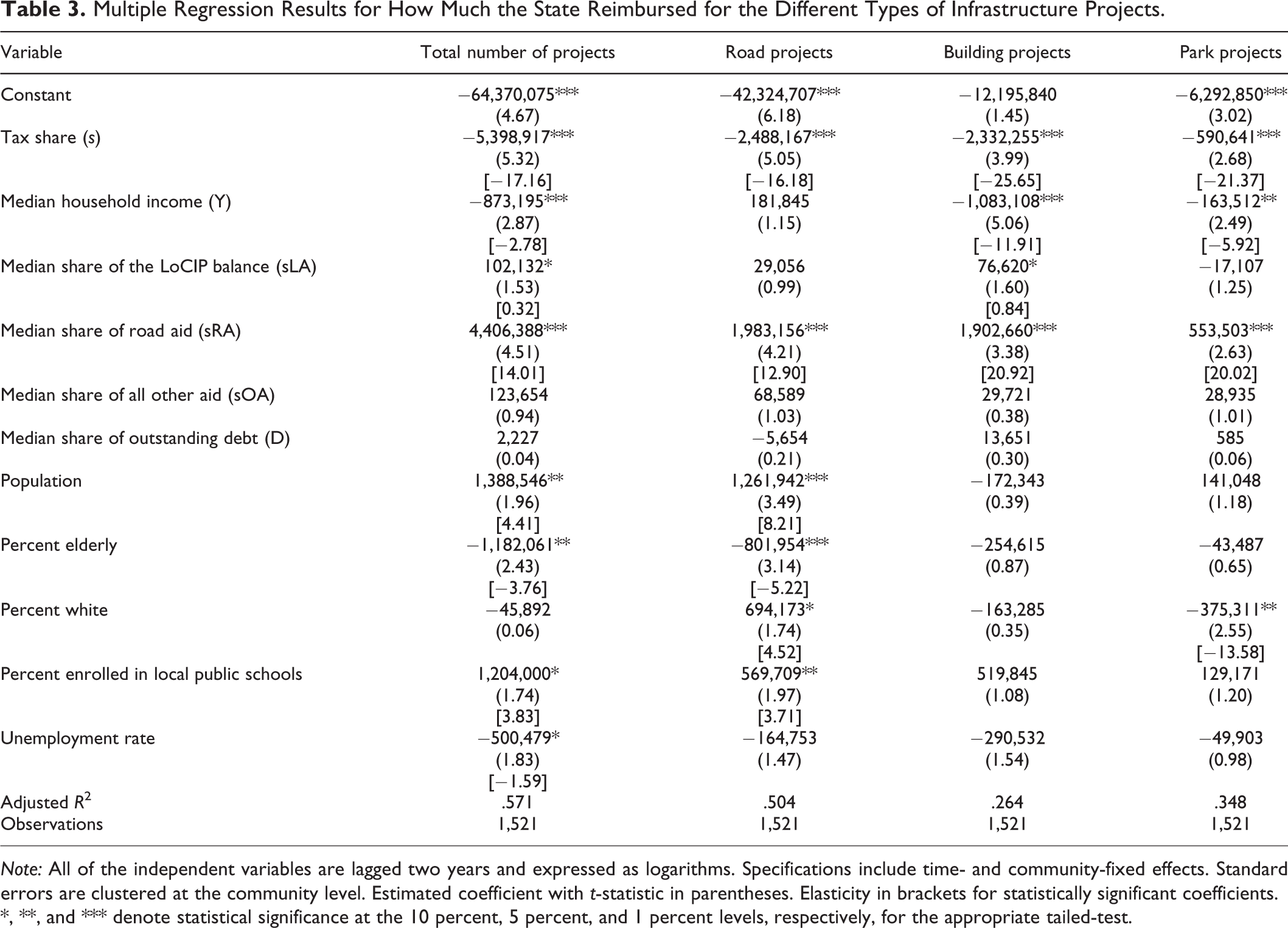
The multiple regression results, associated with using the reimbursed amount as the measure of I for the various types of capital projects, are shown in table 3. The results are reasonably similar to those shown in table 2. For example, the local demands for the various types of capital infrastructure projects are highly elastic with respect to tax share for all four cases. One difference, however, is that the demand for building appears to be the most elastic with respect to tax share.

Table 3.

Multiple Regression Results for How Much the State Reimbursed for the Different Types of Infrastructure Projects.

Variable	Total number of projects	Road projects	Building projects	Park projects
Constant	−64,370,075*** (4.67)	−42,324,707*** (6.18)	−12,195,840 (1.45)	−6,292,850*** (3.02)
Tax share (s)	−5,398,917*** (5.32)	−2,488,167*** (5.05)	−2,332,255*** (3.99)	−590,641*** (2.68)
Tax share (s)	[−17.16]	[−16.18]	[−25.65]	[−21.37]
Median household income (Y)	−873,195*** (2.87)	181,845 (1.15)	−1,083,108*** (5.06)	−163,512** (2.49)
Median household income (Y)	[−2.78]	181,845 (1.15)	[−11.91]	[−5.92]
Median share of the LoCIP balance (sLA)	102,132* (1.53)	29,056 (0.99)	76,620* (1.60)	−17,107 (1.25)
Median share of the LoCIP balance (sLA)	[0.32]	29,056 (0.99)	[0.84]	−17,107 (1.25)
Median share of road aid (sRA)	4,406,388*** (4.51)	1,983,156*** (4.21)	1,902,660*** (3.38)	553,503*** (2.63)
Median share of road aid (sRA)	[14.01]	[12.90]	[20.92]	[20.02]
Median share of all other aid (sOA)	123,654 (0.94)	68,589 (1.03)	29,721 (0.38)	28,935 (1.01)
Median share of outstanding debt (D)	2,227 (0.04)	−5,654 (0.21)	13,651 (0.30)	585 (0.06)
Population	1,388,546** (1.96)	1,261,942*** (3.49)	−172,343 (0.39)	141,048 (1.18)
Population	[4.41]	[8.21]	−172,343 (0.39)	141,048 (1.18)
Percent elderly	−1,182,061** (2.43)	−801,954*** (3.14)	−254,615 (0.87)	−43,487 (0.65)
Percent elderly	[−3.76]	[−5.22]	−254,615 (0.87)	−43,487 (0.65)
Percent white	−45,892 (0.06)	694,173* (1.74)	−163,285 (0.35)	−375,311** (2.55)
Percent white	−45,892 (0.06)	[4.52]	−163,285 (0.35)	[−13.58]
Percent enrolled in local public schools	1,204,000* (1.74)	569,709** (1.97)	519,845 (1.08)	129,171 (1.20)
Percent enrolled in local public schools	[3.83]	[3.71]	519,845 (1.08)	129,171 (1.20)
Unemployment rate	−500,479* (1.83)	−164,753 (1.47)	−290,532 (1.54)	−49,903 (0.98)
Unemployment rate	[−1.59]	−164,753 (1.47)	−290,532 (1.54)	−49,903 (0.98)
Adjusted R ²	.571	.504	.264	.348
Observations	1,521	1,521	1,521	1,521

Note: All of the independent variables are lagged two years and expressed as logarithms. Specifications include time- and community-fixed effects. Standard errors are clustered at the community level. Estimated coefficient with t-statistic in parentheses. Elasticity in brackets for statistically significant coefficients.

*, **, and *** denote statistical significance at the 10 percent, 5 percent, and 1 percent levels, respectively, for the appropriate tailed-test.

The general similarity of the results does not end there. The results depicted in table 3 also show that an increase in median-voter income does not result in a greater demand for the different types of capital infrastructure projects. In fact, the negative coefficient estimate on median household income suggests that the demands for all of the capital projects, except road improvements, are inversely related to changes in income, perhaps indicating that capital infrastructure projects are inferior goods. However, this inverse relationship more likely reflects that wealthier communities rely less on intergovernmental aid when financing local construction projects.

Also, similar to the results in table 2, road aid appears to finance other types of capital projects. Other aid, such as grants for local current school spending, appears to stick more where it initially hits. Other similarities to report are the unimportance of outstanding debt and the general insignificance of the demographic variables. All in all, it appears that the number of capital projects offers a suitable measure of the demand for capital infrastructure projects at least in the context of the LoCIP in Connecticut.

Conclusion

Numerous studies have investigated the demand for current local public spending whereas only a handful of studies have focused on the demand for capital infrastructure projects at the local government level. This study fills a void in the literature by providing useful information to state and local policy makers regarding the demand for different types of municipal infrastructure projects. Specifically, a panel data set of Connecticut towns and cities over the period from 2000 to 2010 is used to estimate the demand for the total number of capital infrastructure projects as well as the individual demands for road, building, and park investment projects. The empirical analysis is based upon a median-voter model of local government decision making. Community- and time-fixed effects are specified to control for unobservable heterogeneity and time trends common to all Connecticut communities. Several valuable insights can be drawn from the empirical analysis.

First, unlike the demands for different types of current spending, the demands for municipal infrastructure projects are found to be unaffected by community income. Often “a rising tide can be expected to raise all ships,” but this finding may indicate that a booming local labor market does not necessarily imply that internal funds will naturally trickle down to finance municipal capital projects. If so, more intergovernmental aid directed at capital projects may be necessary if regional or state authorities believe the current level of municipal capital spending has failed to catch up to the socially efficient level.

Second, the demands for various types of capital infrastructure projects appear to be much more elastic than current spending with respect to tax share. This contrast may mean that a higher tax share often leads to some municipal capital spending being squeezed out as a way of maintaining the consumption levels of current local public goods such as education and police protection. Third, the demands for various types of capital infrastructure projects appear to be relatively sensitive to intergovernmental aid, but the specific type of aid doesn’t always seem to stick where it initially hits. Finally, the age distribution, racial composition, and state of the economy (i.e., unemployment rate) within a community do not seem to exert much impact on the demand for municipal capital infrastructure projects, at least at the margin.

Footnotes

Acknowledgments

We thank Facundo Dominguez and Rudi Wittke of the Connecticut Department of Transportation, Shirley Corona; Sandra Huber and William Plummer of the Connecticut Office of Policy and Management; and Dale Shannon of CERC, Inc., for providing the data used in this study. Santerre also thanks the Center for Real Estate and Urban Economic Studies at the University of Connecticut for funding his participation on this project. The anonymous referee is also thanked for providing valuable comments.

Declaration of Conflicting Interests

The author(s) declared no potential conflicts of interest with respect to the research, authorship, and/or publication of this article.

Funding

The author(s) disclosed receipt of the following financial support for the research, authorship, and/or publication of this article: Rexford E. Santerre received funding from the Center for Real Estate and Urban Economic Studies at the University of Connecticut.

Notes

References

Aschauer

David A.

1989. “Is Public Expenditure Productive?” Journal of Monetary Economics 23:177–200.

Balsdon

Brunner

Eric J.

Rueben

Kim

. 2003. “Private Demand for Public Capital: Evidence from School Bond Referenda.” Journal of Urban Economics 54:610–38.

Bates

Laurie J.

Santerre

Rexford E.

. 2013. “Does Regionalization of Public Health Services Influence Public Spending Levels and Allocative Efficiency?” Regional Science and Urban Economics 43:209–19.

Bergstrom

Theodore C.

Goodman

Robert P.

. 1973. “Private Demands for Public Goods.” The American Economic Review 63:280–96.

Borcherding

Thomas E.

Deacon

Robert

. 1972. “The Demand for the Services of Non-federal Governments.” The American Economic Review 62:891–901.

Bowen

Howard R.

1943. “The Interpretation of Voting in the Allocation of Economic Resources.” Quarterly Journal of Economics 58:27–48.

Brasington

David M.

1999. “Joint Provision of Public Goods: The Consolidation of School Districts.” Journal of Public Economics 73:373–93.

Downs

Anthony

. 1957. An Economic Theory of Democracy. New York: Harper and Row.

Ferris

James M.

Graddy

Elizabeth

. 1994. “Organizational Choice for Public Service Supply.” The Journal of Law, Economics, and Organization 10:126–41.

10.

Ferris

James M.

Graddy

Elizabeth

. 1998. “Production Choices for Local Government Services.” Journal of Urban Affairs 10:251–68.

11.

Haughwout

Andrew F.

1997. “Central City Infrastructure Investment and Suburban House Values.” Regional Science and Urban Economics 27:199–215.

12.

Holtz-Eakin

Douglas

. 1991. “Bond Market Conditions and State-local Capital Spending.” National Tax Journal 44:105–20.

13.

Holtz-Eakin

Douglas

Rosen

Harvey S.

. 1989. “The “Rationality” of Municipal Capital Spending: Evidence from New Jersey.” Regional Science and Urban Economics 19:517–36.

14.

Holtz-Eakin

Douglas

Rosen

Harvey S.

. 1993. “Municipal Construction Spending: An Empirical Examination.” Economics and Politics 5:61–84.

15.

Munnell

Alicia H.

1990. “How Does Public Infrastructure Affect Regional Economic Performance?” New England Economic Review (Federal Reserve Bank of Boston) 6:11–32.

16.

Munnell

Alicia H.

1992. “Policy Watch: Infrastructure Investment and Economic Growth.” The Journal of Economic Perspectives 6:189–98.

17.

Pagano

Michael A.

2002. “Municipal Capital Spending during the “Boom.” Public Budgeting and Finance 22:1–20.

18.

Romer

Thomas

Rosenthal

Howard

. 1979. “The Elusive Median Voter.” Journal of Public Economics 12:143–70.

19.

Temple

Judy

. 1994. “The Debt/Tax Choice in the Financing of State and Local Capital Expenditures.” Journal of Regional Science 34:529–47.

20.

US Department of the Treasury. 2012. “A New Economic Analysis of Infrastructure Investment. A Report Prepared by the Department of the Treasury with the Council of Economic Advisors.” March 23, 2012. http://www.treasury.gov/resource-center/economic-policy/Documents/20120323InfrastructureReport.pdf. Accessed on February 20, 2014.

21.

US Conference of Mayors. 2008. Local Government Investment in Water and Sewer Infrastructure: Adding Value to the National Economy. http://www.usmayors.org/urbanwater/documents/LocalGovt%20InvtInMunicipalWaterandSewerInfrastructure.pdf. Accessed on March 20, 2014.

22.

Wooldridge

J. M.

2002. Econometric Analysis of Cross Section and Panel Data. Cambridge: The MIT Press.

23.

Zimmer

Ron

Buddin

Richard

Jones

John

Liu

. 2011. “What Types of School Capital Projects Are Voters Willing to Support?” Public Budgeting and Finance 31:37–55.