Precautionary Social Planning

Abstract

It is a truism of neoclassical economics that a sufficiently high savings rate will be bad if it is dynamically inefficient. Here we consider a Solow model in which households follow a savings rate dictated by a social planner. Ideally, the social planner would instruct households to save at the Golden Rule savings rate that maximizes consumption per capita, but this advice needs to be adjusted when the social planner has imperfect control over how much households actually save. Analogous to what happens with precautionary saving at the household level, in this case, the social planner will maximize social welfare by targeting a savings rate higher than the Golden Rule. Precautionary social planning then yields a dynamically inefficient allocation, albeit with greater stability of consumption, which is often a stated priority of social planners.

Keywords

Solow model optimal irrational behavior precautionary motive social planner efficiency/stability tradeoff

The workhorse models that currently predominate macroeconomics and public finance started to be developed in the 1950s when the United States had the largest economy in the world, so, naturally, the United States was the prototypical country that these models were constructed to describe. Today, however, the world is undergoing a massive geopolitical transition. Depending on how one compares gross domestic product (GDP) across countries, China is now either the largest or second-largest economy on the planet, and within a few years there will be no ambiguity. A large literature models China like we would model the United States: as a country of decentralized rational households who each individually maximize their utility subject to budget constraints in a pure market economy.¹ However, the question needs to be asked whether this is the most appropriate way to model China. In liberal democracies, it is quite reasonable to assume that households behave with virtual autonomy since that is the fundamental nature of liberal democracy. China, in contrast, impugns the social instability that it claims results from giving individuals too much freedom.

The aggregate savings rate for China averaged to 40 percent between 2002 and 2020.² This is a much higher rate than what we typically observe in liberal democracies, and it is very difficult to explain with a decentralized model. For example, Song, Storesletten, and Zilibotti (2011) have to assume households are extremely patient with a discount rate of 0.3 percent, which is an order of magnitude smaller than what we usually assume for Western economies, when constructing a decentralized growth model consistent with Chinese macroeconomic data.³ Another framework we could use to study China, one that requires fewer assumptions, is the Solow (1956) model with an endogenous savings rate. It seems much more plausible to suppose that China’s leaders are coordinating household behavior to generate high savings than it is to suppose that Chinese households are independently choosing to save more than their Western counterparts. If a social planner chooses a target savings rate to maximize its objectives—which is literally what China purports to do with its five-year plans⁴ —it is actually quite easy to understand why China would save at the Golden Rule savings rate that maximizes steady-state consumption per capita.

Some critics will argue that the Solow model is too simple for use by economists today. It would be more accurate to say that the Solow model is too simple to address most questions that Western economists have about how economic issues impact voters. The Cass–Koopmans–Ramsey model,⁵ overlapping-generations models,⁶ and their various successors did not supplant the Solow model because of their empirical successes. All of these models are about equally good—or bad—at forecasting.⁷ They are useful because they can predict how households will respond to changes in public policy, which the Solow model cannot. But in the present context, where we are asking questions about decision-making at the societal level rather than at the individual level, we do not require the sophistication of these more popular models. If we can obtain a plausible explanation for China’s savings rate without assuming a pure market economy with perfectly rational households, then Occam’s Razor will favor the model that makes fewer assumptions. Since we are focusing only on aggregate behavior, we can abstract from how individual decisions are made and represent the aggregate of their behavior as noise.⁸ The central ingredients of this stripped-down model are the production function and the process for determining the aggregate savings rate. We do not even have to distinguish between public and private goods.⁹

The predominant question for most economists trying to understand China today is whether it is saving too much. This is based on an intuition that derives from neoclassical models with utility-maximizing households. Recent five-year plans have put more emphasis on encouraging consumption, suggesting that China’s leaders are also worried that the country has been saving too much. Notwithstanding these sentiments, we can calibrate our model so that China is saving the right amount.¹⁰ There are also calibrations where China could achieve its societal goals more expeditiously by saving more.

While there are Keynesian concerns about Chinese oversaving that we do not consider here, the neoclassical argument is that China’s economy may be dynamically inefficient. However, the concept of Pareto efficiency is only relevant in a context where the social planner, whether putative or real, has absolute control over the allocation of goods.¹¹ In a pure command economy where the social planner only cares about consumption in the steady state, as a social planner ought to according to Ramsey (1928), he would trivially choose the Golden Rule savings rate that maximizes steady-state consumption. Things are more complicated in a slightly mixed economy approximate to a command economy, which we model by allowing noisy household behavior to interfere with the social planner’s control over the aggregate savings rate. Then we can also account for deviations of the target savings rate from the Golden Rule. The social planner will have a precautionary motive to save more or less than the Golden Rule,¹² depending on the parameters of the production function.

As in Leland (1968) and Sandmo (1970), the optimal savings target will depend on the third derivative of the social planner’s objective function. If the third derivative is positive, consumption will decline more from its maximum if households save too little than if they save too much. Consequently, it will be optimal for the social planner to target a savings rate that, at least ostensibly, is dynamically inefficient. Given reasonable assumptions about the utility function, for small noise variances, the optimal adjustment of the savings target from the Golden Rule does not depend on the choice of a utility function. The third derivative of steady-state consumption is strictly a function of the third and lower derivatives of the production function at the Golden Rule steady state. In general, the condition for dynamic inefficiency relates the elasticity corresponding to this third derivative to the elasticity of substitution between capital and labor.

For the case of a Cobb–Douglas production function, the Golden Rule savings rate is the (constant) share of capital, and the third derivative of consumption will be positive if the share of capital is less than one-half. If we generalize to a constant elasticity of substitution (CES) production function, the Golden Rule savings rate will depend on both the parameters of the production function and the growth (or decay) rates of the factors of production. The range of Golden Rule savings rates for which dynamic efficiency is optimal depends on the elasticity of substitution between capital and labor. The more complementary capital and labor are, the larger this range will be. This follows because, if the elasticity of substitution is less than one and households do not save enough to maintain enough capital to produce, consumption will converge to zero. The social planner will very much want to avoid this outcome, so the precautionary motive to save more will become especially strong as the elasticity of substitution decreases. If the elasticity is less than 0.5, dynamic inefficiency is always optimal. In contrast, if capital and labor are highly substitutable, capital is not essential for production so a low savings rate is less terrible. In the limit where capital and labor are nearly perfect substitutes, dynamic inefficiency will only be optimal if the Golden Rule savings rate is greater than 20 percent.

For the motivating case of China, the aggregate savings rate has averaged 40 percent in recent years and the income share of capital has averaged 0.5.¹³ Taken at face value, these numbers suggest that China ought to be saving in the vicinity of 50 percent. However, what matters is the share of capital at the steady state, not the share of capital during the transition. If, as China builds up its capital stock, the share of capital drops to the range of 0.3–0.4 like for most developed countries today, a savings rate of 40 percent could be optimal. In a model calibrated to match current Chinese macroeconomic data, we find this can happen if the elasticity of substitution between capital and labor is roughly between 0.7 and 0.8.

The paper is organized as follows. In section “The Model,” we describe the model. In section “The Golden Rule,” we review the Golden Rule, which will give the optimal savings rate in a pure command economy where the social planner has perfect control over households. In section “General Results with Imperfect Control,” we generalize to the case where the social planner has imperfect control. In sections “Cobb–Douglas Production” and “CES Production,” we discuss what happens for the particular cases of a Cobb–Douglas and CES production function, respectively. In section “Application to China,” we calibrate the model so China’s current savings rate is optimal. We conclude in the “Concluding Remarks” section.

The Model

Our object of study is a closed economy with a constant returns to scale aggregate production function

Y (t) = F (K (t), A (t) L (t))

(1)

of the factors of production capital

K (t)

, labor

L (t)

, and labor-augmenting technology

A (t)

. We assume that labor and technology grow exogenously at the rates

n

and

g

, respectively, and capital depreciates exogenously at the rate

δ

. If we define capital per effective labor

k (t) = \frac{K (t)}{A (t) L (t)},

(2)

and the intrinsic production function

f (k) = F (k, 1),

(3)

we can rewrite the production function as

Y (t) = A (t) L (t) f (k (t)) .

We also assume the function

f (k)

is positive, strictly increasing, and strictly concave; has a continuous third derivative for

k > 0

; and is nonnegative for

k = 0

. It is helpful to define

ξ = n + g + δ,

(4)

which we assume is positive. This is the unit cost of maintaining a constant capital per effective labor. We also assume that

lim_{k \to \infty} f^{'} (k) < ξ < lim_{k \to 0} f^{'} (k) .

(5)

Most of the other assumptions of a macro model relate to how final goods will be divvied up between various end users. Here we only distinguish between whether a final good is installed as capital or consumed so we can dispense with those assumptions. We have

Y (t) = C (t) + I (t),

(6)

where

C (t)

includes both public and private consumption and

I (t)

includes both public and private investment. Investment adds to the capital stock, yielding the equation of motion

\frac{d K (t)}{d t} = I (t) - δ K (t) .

(7)

The main innovation of the paper is to assume that the savings rate

s \in (0, 1)

, such that

I (t) = s Y (t),

(8)

is determined by a social planner so as to maximize a social welfare function. We can then differentiate

k (t)

to obtain the familiar Solow equation of motion

\frac{d k (t)}{d t} = s f (k (t)) - ξ k (t) .

(9)

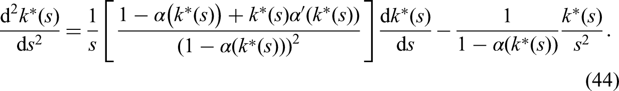
Suppose that

s

is large enough that there exists

\underline{k} \geq 0

such that

s f (\underline{k}) > ξ \underline{k}

.¹⁴ Then (5) implies that a

k^{*} (s) > \underline{k}

will exist such that

s f (k^{*} (s)) = ξ k^{*} (s),

(10)

and the strict concavity of

f

implies that

k^{*} (s)

must be unique.¹⁵ For any

k (0) \geq \underline{k}

, the resulting solution to (9) will satisfy

lim_{t \to \infty} k (t) = k^{*} (s)

. Given our assumptions about the smoothness of

s

k^{*} (s)

must be continuous and thrice differentiable. Let us then define

c^{*} (s) = (1 - s) f (k^{*} (s))

(11)

as steady-state consumption per effective labor, which is also continuous and thrice differentiable.

While the original Solow (1956) paper treated the savings rate $s$ as exogenous, here we endogenize $s$ . The social planner chooses its target savings rate $\tilde{s}$ to maximize

V (\tilde{s}) = E [u (c^{*} (\tilde{s} + ε))],

(12)

where

u (c)

is a strictly concave, strictly increasing function with a continuous third derivative for

c > 0

; the actual savings rate is

s = \tilde{s} + ε

; and

ε

is a mean-zero noise variable with variance

V [ε] = τ^{2}

.¹⁶ Note that this differs substantially from the common utilitarian social welfare function which is a weighted sum of the utilities of individual households. Indeed, there need not be any connection between the social planner’s utility function and that of households. What ultimately matters to the social planner is

s

, but, if

τ > 0

, the social planner will not have complete control over

s

Our approach, while unusual, is consistent with what many socialists advocate. In his “Critique of the Gotha Program,” Marx (1875) famously summarized the long-run goal of communism to be that consumption should be allocated such that “From each according to his ability, to each according to his needs!” Since it would be impossible for a social planner to anticipate all of the future needs of households, the objective should presumably be to maximize the size of the pie available to accommodate those needs, that is, to maximize the available aggregate consumption, which $c^{*}$ is proportional to. By focusing on the steady state, we also effectively weigh all generations the same, avoiding the ethical dilemma of having to play favorites between generations.¹⁷ On the other side, this choice of social welfare function also means the social planner does not care a whit about the Pareto criterion for ranking allocations. Only in the special case where all households have exactly the same preferences as the social planner should we expect equilibrium allocations to be Pareto efficient.¹⁸

The noise $ε$ in the savings rate arises because the social planner does not have full control in coordinating the behavior of households. We simply leave the variance $τ^{2}$ exogenous since it is not a subject of our inquiry. Households with preferences similar to what is normally employed in neoclassical models will almost surely have an incentive to deviate from the behavior prescribed by the social planner so the variance of $ε$ will increase as households are more willing to act independently. But even if households are entirely docile, coordination failures may still occur, resulting in a positive $τ$ .¹⁹

To connect what we are doing with a more traditional macro model, we can suppose that we have $M$ households such that the $i$ th household earns labor income $y_{t}^{i}$ at $t$ and has previously accumulated savings $b_{t}^{i}$ that earns the interest rate $r_{t}$ . Normally, we would assume the household will choose its consumption $c_{t}^{i}$ and save for the next period $b_{t + 1}^{i}$ to maximize a utility function subject to the budget constraint

c_{t}^{i} + b_{t + 1}^{i} = y_{t}^{i} + (1 + r_{t}) b_{t}^{i} .

(13)

Then next period’s capital stock is determined by aggregating the savings

K_{t + 1} = \sum_{i = 1}^{M} b_{t + 1}^{i} .

(14)

What we are doing in essence is to assume that for household

i

there is some stochastic distribution for its saving

b_{t + 1}^{i}

that depends on the social planner’s target savings rate

\tilde{s}

. If we define the average labor income

{\bar{y}}_{t} = \frac{1}{M} \sum_{i = 1}^{M} y_{t}^{i}

(15)

and average savings

{\bar{b}}_{t} = \frac{1}{M} \sum_{i = 1}^{M} b_{t}^{i},

(16)

there will be some

s

that satisfies²⁰

{\bar{b}}_{t + 1} = s ({\bar{y}}_{t} + (r_{t} + δ) {\bar{b}}_{t}) + (1 - δ) {\bar{b}}_{t} .

(17)

Thus the distribution of

ε = s - \tilde{s}

could be derived from the distributions of the

b_{t + 1}^{i}

, although we do not bother to do that here.

However the $b_{t + 1}^{i}$ are chosen, we could always solve (17) for $s$ . The only actual content to the assumptions we are making here is that $s$ remains constant in time.²¹ For an economy where there is a central authority, it seems more sensible to assume the planner will try to induce households to follow

b_{t + 1}^{i} = \tilde{s} (y_{t}^{i} + (r_{t} + δ) b_{t}^{i}) + (1 - δ) b_{t}^{i}

(18)

then to assume each household maximizes its utility without any coordination.²²

The Golden Rule

We begin by reviewing the familiar textbook example of the model without uncertainty. In that case, the social planner’s objective function reduces to $V (\tilde{s}) = U (\tilde{s})$ , where

U (s) = u (c^{*} (s)) .

(19)

The first-order condition for the social planner’s problem is

U^{'} (s) = u^{'} (c^{*} (s)) \frac{d c^{*} (s)}{d s} = 0.

(20)

Since

u

is strictly increasing, the social planner needs to find a solution to

d c^{*} (s) / d s = 0

, what is commonly known as the Golden Rule savings rate.

The steady state is defined by (10), so we can rewrite steady-state consumption as a function of $k^{*}$ alone:

c^{*} (s) = f ((k^{*} (s)) - ξ k^{*} (s) .

(21)

Thus

\frac{d c^{*} (s)}{d s} = [f^{'} (k^{*} (s)) - ξ] \frac{d k^{*} (s)}{d s} .

(22)

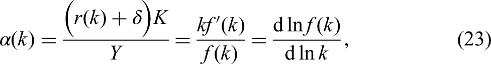
Let us define the share of capital as

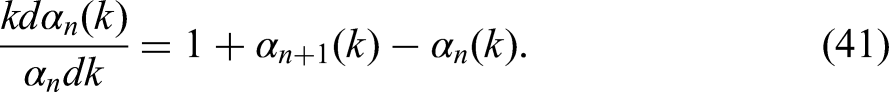
α (k) = \frac{(r (k) + δ) K}{Y} = \frac{k f^{'} (k)}{f (k)} = \frac{d \ln f (k)}{d \ln k},

(23)

which is between zero and one since

f

is strictly increasing and strictly concave. Implicit differentiation of (10) yields a derivative of

k^{*} (s)

that can be written in terms of the share of capital as

\frac{d k^{*} (s)}{d s} = \frac{1}{1 - α (k^{*} (s))} \frac{k^{*} (s)}{s},

(24)

which is strictly positive if

s, k^{*} (s) > 0

, in which case the corresponding elasticity works out very simply to

\frac{d \ln k^{*} (s)}{d \ln s} = \frac{1}{1 - α (k^{*} (s))} > 0.

(25)

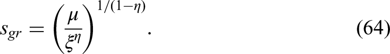
As we will shortly corroborate,

c^{*} (s)

has a global maximum at s_{g
r} by (22) satisfies

f^{'} (k^{*} (s_{g r})) = ξ,

(26)

or equivalently, using (23) and (10)

α (k^{*} (s_{g r})) = s_{g r} .

(27)

Thus the Golden Rule savings rate will in fact equal the share of capital at the Golden Rule steady state.

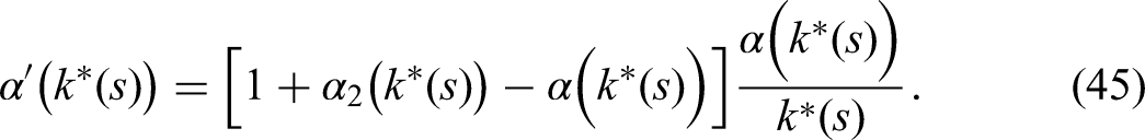
Note that $s_{g r}$ is indeed a maximum of $U (s)$ . The second derivative is

U^{″} (s) = u^{″} (c^{*} (s)) {(\frac{d c^{*} (s)}{d s})}^{2} + u^{'} (c^{*} (s)) \frac{d^{2} c^{*} (s)}{d s^{2}} .

(28)

Since

u

is strictly concave, the first term is unambiguously negative for all

s

. Differentiating (22) again,

\frac{d^{2} c^{*} (s)}{d s^{2}} = f^{″} (k^{*} (s)) {(\frac{d k^{*} (s)}{d s})}^{2} + [f^{'} (k^{*} (s)) - ξ] \frac{d^{2} k^{*} (s)}{d s^{2}},

(29)

\frac{d^{2} c^{*} (s_{g r})}{d s^{2}} = f^{″} (k^{*} (s_{g r})) {(\frac{d k^{*} (s_{g r})}{d s})}^{2} < 0.

(30)

Thus at the Golden Rule savings rate, the second term of (28) is also negative, so

U^{″} (s_{g r}) < 0

. In the absence of uncertainty, the solution to the social planner’s problem is to set the savings rate equal to the share of capital.

The preceding treatment, however, is quite different from how one normally investigates this model. Instead, the focus is usually on which savings rates generate allocations that are Pareto inefficient regardless of preferences. While $U (0)$ and $U (1)$ may not be defined, clearly $c^{*} (0) = c^{*} (1) = 0$ . Since $c^{*} (s)$ is continuous, if $s \in (s_{g r}, 1)$ , there must exist $s^{'} \in (0, s_{g r})$ such that $c^{*} (s) = c^{*} (s^{'})$ . However, $k^{*} (s) > k^{*} (s^{'})$ . Thus if the economy consumes $k^{*} (s) - k^{*} (s^{'})$ in an instant, it will immediately be able to resume a stable trajectory with a new steady-state capital per effective labor $k^{*} (s^{'})$ while maintaining the same steady-state consumption per effective labor $c^{*} (s)$ as before. Since by this transition from the steady state with savings rate $s$ to a savings rate $s^{'}$ it is possible to increase consumption at one instant while maintaining the same consumption at all other instants, an economy with savings rate $s > s_{g r}$ is said to be dynamically inefficient.

What often goes unnoticed in discussing dynamic inefficiency, though, is that the possibility of costless improvement will be purely hypothetical if the economy is not able to precisely adjust its savings rate. In the following, we relax the assumption that the social planner has perfect control over the savings rate.

General Results with Imperfect Control

The main innovation of the paper is to suppose that a real-world social planner may not have perfect control over the behavior of his charges. If the social planner can choose a target savings rate $\tilde{s}$ , but the actual aggregate savings rate $s = \tilde{s} + ε$ , where $ε$ is a mean-zero noise variable, then the social planner’s objective function will be

V (\tilde{s}) = E [U (\tilde{s} + ε)] .

(31)

We are not interested in a figurehead social planner. The actual savings rate should be reasonably close to the target savings rate, so we assume the variance

τ^{2}

is small compared to one.²³

The social planner will optimally choose $\tilde{s}$ so that

V^{'} (\tilde{s}) = E [U^{'} (\tilde{s} + ε)] = 0.

(32)

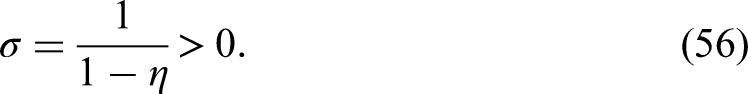
We will treat the dimensionless

τ

as a perturbation parameter around the optimal choice of

\tilde{s} = s_{g r}

when

τ = 0

. Then the

n

th moment of

ε

will be to

n

th order in

τ

unless the moment vanishes. Let us define

Δ s = \tilde{s} - s_{g r} .

(33)

Since

Δ s

vanishes when

τ = 0

Δ s

must be at least first order in

τ

. A Taylor expansion of (32) to second order in

τ

yields

E [U^{'} (s_{g r}) + U^{″} (s_{g r}) (Δ s + ε) + \frac{1}{2} U^{″'} (s_{g r}) (Δ s + ε)^{2}] + O (τ^{3}) = 0,

(34)

which simplifies to

U^{″} (s_{g r}) Δ s + \frac{1}{2} U^{″'} (s_{g r}) (Δ s^{2} + τ^{2}) + O (τ^{3}) = 0.

(35)

Note that if

Δ s

is first order in

τ

U^{″} (s_{g r}) Δ s

would be the only first-order term in (35). Since

U^{″} (s_{g r}) < 0

, any first-order contribution to

Δ s

must vanish. Therefore, we can disregard the

Δ s^{2}

term in (35) since it must be to fourth order in

τ

. We are left with

U^{″} (s_{g r}) Δ s + \frac{1}{2} U^{″'} (s_{g r}) τ^{2} + O (τ^{3}) = 0,

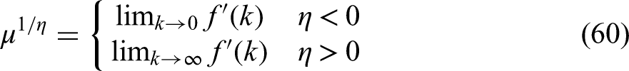
which gives that the optimal buffer between the target savings rate and the Golden Rule savings rate is

Δ s = - \frac{1}{2} \frac{U^{″'} (s_{g r})}{U^{″} (s_{g r})} τ^{2} + O (τ^{3}) .

(36)

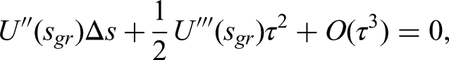
The minus sign is cancelled by the negative

U^{″} (s_{g r})

, so

Δ s

has the same sign as

U^{″'} (s_{g r})

. If

U^{″'} (s_{g r}) > 0

U

will decline more slowly as we move away from

s_{g r}

to the right than if we move away from

s_{g r}

to the left. Erring on the side of caution, the social planner should choose

\tilde{s} > s_{g r}

with

Δ s

proportional to the variance of

ε

. Conversely, if

U^{″'} (s_{g r}) < 0

, he should do the opposite.²⁴

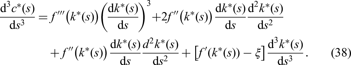
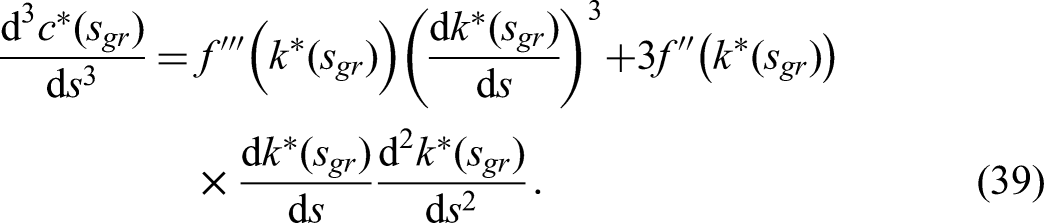
Thus everything for the social planner hinges on the third derivative of $U$ at the Golden Rule. Since

U^{″'} (s) = u^{″'} (c^{*} (s)) {(\frac{d c^{*} (s)}{d s})}^{3} + 3 u^{″} (c^{*} (s)) \frac{d c^{*} (s)}{d s} \frac{d^{2} c^{*} (s)}{d s^{2}} + u^{'} (c^{*} (s)) \frac{d^{3} c^{*} (s)}{d s^{3}},

(37)

this works out to

U^{″'} (s_{g r}) = u^{'} (c^{*} (s_{g r})) \frac{d^{3} c^{*} (s_{g r})}{d s^{3}} .

We have assumed marginal utility is positive, so the sign of the third derivative of

U

is completely independent of the utility function

u

. Actually, (28) evaluated at

s_{g r}

implies that all appearances of the utility function

u

disappear from (36), so the magnitude of the optimal

Δ s

also does not depend on

u

to second order in

τ

Differentiating (29) once more,

\begin{aligned} \frac{d^{3} c^{*} (s)}{d s^{3}} & = f^{″'} (k^{*} (s)) {(\frac{d k^{*} (s)}{d s})}^{3} + 2 f^{″} (k^{*} (s)) \frac{d k^{*} (s)}{d s} \frac{d^{2} k^{*} (s)}{d s^{2}} \\ + f^{″} (k^{*} (s)) \frac{d k^{*} (s)}{d s} \frac{d^{2} k^{*} (s)}{d s^{2}} + [f^{'} (k^{*} (s)) - ξ] \frac{d^{3} k^{*} (s)}{d s^{3}} . \end{aligned}

(38)

At the Golden Rule savings rate, this reduces to

\frac{d^{3} c^{*} (s_{g r})}{d s^{3}} = f^{″'} (k^{*} (s_{g r})) {(\frac{d k^{*} (s_{g r})}{d s})}^{3} + 3 f^{″} (k^{*} (s_{g r})) \frac{d k^{*} (s_{g r})}{d s} \frac{d^{2} k^{*} (s_{g r})}{d s^{2}} .

(39)

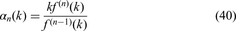
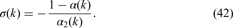
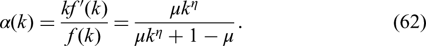
This third derivative can be expressed most transparently in terms of the elasticities of the production function. We define

α_{n} (k) = \frac{k f^{(n)} (k)}{f^{(n - 1)} (k)}

(40)

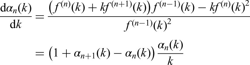
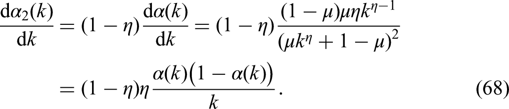
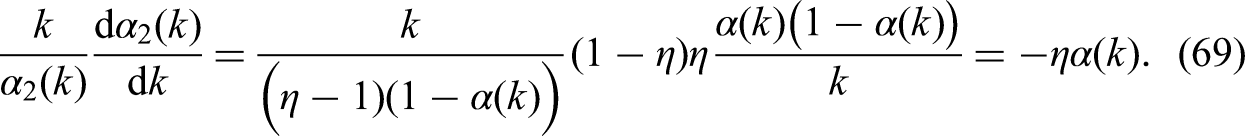
to be the elasticity of the

n

th derivative of the intrinsic production function with respect to capital per effective labor. The derivative of

α_{n} (k)

\begin{aligned} \frac{d α_{n} (k)}{d k} & = \frac{(f^{(n)} (k) + k f^{(n + 1)} (k)) f^{(n - 1)} (k) - k f^{(n)} {(k)}^{2}}{f^{(n - 1)} {(k)}^{2}} \\ = (1 + α_{n + 1} (k) - α_{n} (k)) \frac{α_{n} (k)}{k} \end{aligned}

So the elasticity of

α_{n} (k)

\frac{k d α_{n} (k)}{α_{n} d k} = 1 + α_{n + 1} (k) - α_{n} (k) .

(41)

If we interpret

f^{(0)} (k)

as the production function, then

α_{1} (k)

is the share of capital. The elasticity

α_{2} (k)

is usually interpreted as a dimensionless measure of the curvature of the production function. Let

σ (k)

denote the elasticity of substitution between capital and labor, which, from Feigenbaum (2019), can be written in terms of these elasticities as

σ (k) = - \frac{1 - α (k)}{α_{2} (k)} .

(42)

The geometric interpretation of

α_{3} (k)

is called aberrancy (Schot, 1978). This measures how asymmetric the deviation of the production function is from a quadratic tangent to the production function.

Isolating some unambiguously negative common factors out of (39), we get

\begin{aligned} \frac{d^{3} c^{*} (s_{g r})}{d s^{3}} & = [α_{3} (k^{*} (s_{g r})) \frac{s}{k^{*} (s_{g r})} \frac{d k^{*} (s_{g r})}{d s} + 3 \frac{s}{d k^{*} (s_{g r}) / d s} \frac{d^{2} k^{*} (s_{g r})}{d s^{2}}] \\ \times \frac{f^{″} (k^{*} (s_{g r}))}{s} {(\frac{d k^{*} (s_{g r})}{d s})}^{2} . \end{aligned}

(43)

We have already computed the elasticity of

k^{*}

, so the final ingredient is the elasticity of

d k^{*} (s) / d s

Differentiating (24),

\frac{d^{2} k^{*} (s)}{d s^{2}} = \frac{1}{s} [\frac{1 - α (k^{*} (s)) + k^{*} (s) α^{'} (k^{*} (s))}{(1 - α (k^{*} (s)))^{2}}] \frac{d k^{*} (s)}{d s} - \frac{1}{1 - α (k^{*} (s))} \frac{k^{*} (s)}{s^{2}} .

(44)

We rearrange (41) for

n = 1

to obtain

α^{'} (k^{*} (s)) = [1 + α_{2} (k^{*} (s)) - α (k^{*} (s))] \frac{α (k^{*} (s))}{k^{*} (s)} .

(45)

Substituting in this result and (24)

\begin{aligned} \frac{d^{2} k^{*} (s)}{d s^{2}} & = - \frac{1}{1 - α (k^{*} (s))} \frac{k^{*} (s)}{s^{2}} + [\frac{1}{1 - α (k^{*} (s))} \\ + \frac{[1 + α_{2} (k^{*} (s)) - α (k^{*} (s))] α (k^{*} (s))}{(1 - α (k^{*} (s)))^{2}}] \frac{1}{1 - α (k^{*} (s))} \frac{k^{*} (s)}{s^{2}} \end{aligned}

This simplifies to

\frac{d^{2} k^{*} (s)}{d s^{2}} = [2 + \frac{α_{2} (k^{*} (s))}{1 - α (k^{*} (s))}] \frac{α (k^{*} (s))}{1 - α (k^{*} (s))} \frac{1}{s} \frac{d k^{*} (s)}{d s} .

(46)

Thus the elasticity is

\frac{s}{d k^{*} (s) / d s} \frac{d^{2} k^{*} (s)}{d s^{2}} = \frac{α (k^{*} (s))}{1 - α (k^{*} (s))} [2 + \frac{α_{2} (k^{*} (s))}{1 - α (k^{*} (s))}] .

(47)

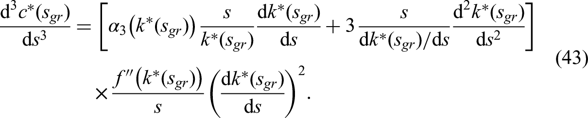
Inserting (25) and (47) into (43), we arrive at our principal result. The third derivative of steady-state consumption per effective labor is

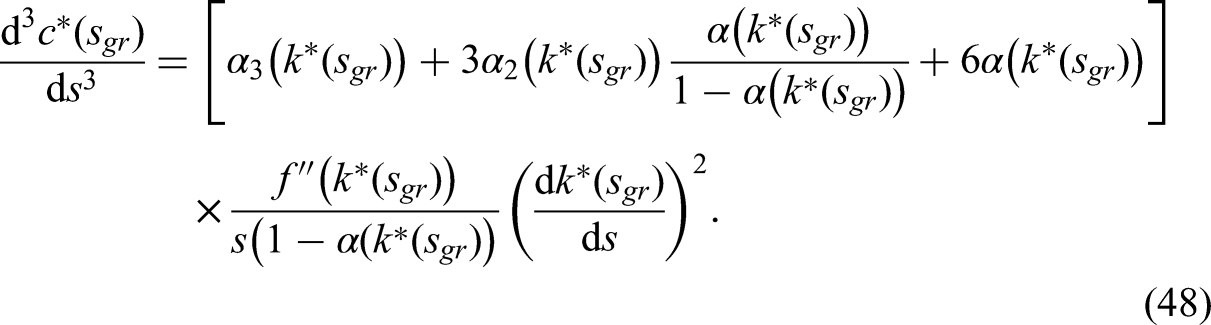
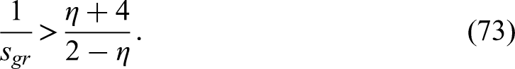
\begin{aligned} \frac{d^{3} c^{*} (s_{g r})}{d s^{3}} & = [α_{3} (k^{*} (s_{g r})) + 3 α_{2} (k^{*} (s_{g r})) \frac{α (k^{*} (s_{g r}))}{1 - α (k^{*} (s_{g r}))} + 6 α (k^{*} (s_{g r}))] \\ \times \frac{f^{″} (k^{*} (s_{g r}))}{s (1 - α (k^{*} (s_{g r}))} {(\frac{d k^{*} (s_{g r})}{d s})}^{2} . \end{aligned}

(48)

Note that the factors outside the brackets are still unambiguously negative. Thus the condition for dynamic inefficiency to be optimal is that

α_{3} (k^{*} (s_{g r})) + 3 α_{2} (k^{*} (s_{g r})) \frac{α (k^{*} (s_{g r}))}{1 - α (k^{*} (s_{g r}))} + 6 α (k^{*} (s_{g r})) < 0.

(49)

Taking (42) into account, we can further simplify the condition to

α_{3} (k^{*} (s_{g r})) < 3 α (k^{*} (s_{g r})) (\frac{1}{σ (k^{*} (s_{g r}))} - 2) .

(50)

Since

α_{3} (k) = k f^{″'} (k) / f^{″} (k)

, this elasticity related to the aberrancy of the production function will be negative if

f^{″'} (k^{*} (s_{g r})) > 0

. Thus (50) means that if the third derivative of the production function at the Golden Rule steady state is sufficiently large then dynamic inefficiency will be optimal. Since the share of capital is positive, the right-hand side of (50) is decreasing in the elasticity of substitution. As capital and labor become more substitutable, the bound on

f^{″'} (k^{*} (s_{g r}))

such that dynamic inefficiency is optimal gets tighter. Conversely, in the limit as capital and labor are perfect complements, dynamic inefficiency will always be optimal. This is a consequence of capital being essential for production when capital and labor are substitutes. If the savings rate is sufficiently low, even though it is positive, households will not be able to maintain a positive capital stock, so the social planner will be strongly incentivized to err on the side of higher savings regardless of other parameters of the production function.

From (36), (29) and (38) imply that the optimal ratio of the buffer between the target savings rate and the Golden Rule savings rate to the variance of $ε$ is in the limit as this variance goes to zero

lim_{τ \to 0} \frac{Δ s}{τ^{2}} = - \frac{1}{2} \frac{α_{3} (k^{*} (s_{g r})) + 3 α_{2} (k^{*} (s_{g r})) [s_{g r} / (1 - s_{g r})] + 6 s_{g r}}{(1 - s_{g r}) s_{g r}} .

(51)

Cobb–Douglas Production

The Cobb–Douglas production function

f (k) = k^{α}

(52)

is the simplest and most commonly used production function precisely because the share of capital

α (k) = α

, which also equals the Golden Rule savings rate, is constant. Indeed, all of the elasticities

α_{n} = α - n + 1

are constant, which follows from induction. If

d α_{k} (k) / d k = 0

, then (41) gives

α_{n + 1} = α_{n} - 1 = α - n + 1 - 1 = α - n .

(53)

The condition (49) then reduces to

α - 2 + 3 (α - 1) \frac{α}{1 - α} + 6 α < 0

4 α < 2 .

Dynamic inefficiency will be socially optimal with Cobb–Douglas production as long as the share of capital is less than one-half.

The optimal ratio of the buffer to the noise variance is for small $τ$

lim_{τ \to 0} \frac{Δ s}{τ^{2}} = - \frac{1}{2} \frac{α - 2 + 3 (α - 1) \frac{α}{1 - α} + 6 α}{(1 - α) α} = - \frac{1}{2} \frac{α - 2 - 3 α + 6 α}{(1 - α) α} = \frac{1 - 2 α}{(1 - α) α} .

(54)

Since

\frac{d}{d α} (\frac{1 - 2 α}{(1 - α) α}) = - \frac{(1 - α)^{2} + α^{2}}{(1 - α)^{2} α^{2}} < 0,

the optimal buffer to variance ratio is strictly decreasing in the share of capital. The buffer will be larger in magnitude the farther that the share of capital gets from one-half.²⁵

CES Production

The situation is more complicated for other members of the larger class of CES production functions. For one thing, not all production functions in this class satisfy both inequalities of the assumption (5). The inhabitants of an economy where the production function violates the inequality for $k \to \infty$ can rejoice because for them economics is not a dismal science. Their economy is a generalization of an $A K$ model with $A > ξ$ , so a high enough savings rate will permit their consumption per effective labor to grow without bound. In contrast, if the production function violates the inequality for $k \to 0$ , no savings rate is high enough to maintain a positive capital stock in the long run.

In this class of production functions

f (k) = [μ k^{η} + 1 - μ]^{1 / η}

(55)

for

η \in (- \infty, 0) \cup (0, 1)

and

μ \in (0, 1)

. The Cobb–Douglas case is nested within this family since, as

η \to 0

f (k) \to k^{μ}

. As we will see below, the elasticity of substitution is, consistent with the name of this class, constant and equal to

σ = \frac{1}{1 - η} > 0 .

(56)

When

η > 0

σ > 1

, so we say in this case that capital and labor are substitutes. When

η < 0

σ < 1

, so we say in this case that capital and labor are complements. In the Cobb–Douglas case of

η = 0

, capital and labor are neither complements nor substitutes.

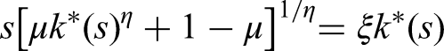
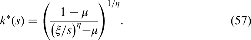
One of the advantages of a CES production function is that we get an analytic solution for the steady-state capital per effective labor. If we raise both sides of the steady-state equation

s {[μ k^{*} {(s)}^{η} + 1 - μ]}^{1 / η} = ξ k^{*} (s)

to the

η

th power, we get an equation linear in

k^{*} {(s)}^{η}

. Thus

k^{*} (s) = {(\frac{1 - μ}{{(ξ / s)}^{η} - μ})}^{1 / η} .

(57)

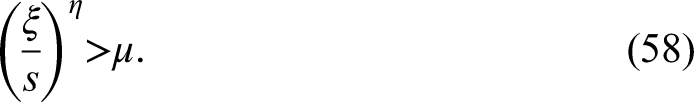
However, this solution is only well-defined if

{(\frac{ξ}{s})}^{η} > μ .

(58)

For

η ≷ 0

, this condition simplifies to

s ≶ ξ / μ^{1 / η}

. Since

f^{'} (k) = μ {(\frac{k}{[μ k^{η} + 1 - μ]^{\frac{1}{η}}})}^{η - 1} = μ {(\frac{k}{f (k)})}^{η - 1},

(59)

the significance of

μ^{1 / η}

is that

μ^{1 / η} = {\begin{matrix} {lim}_{k \to 0} f^{'} (k) & η < 0 \\ {lim}_{k \to \infty} f^{'} (k) & η > 0 \end{matrix}

(60)

η > 0

, the assumption (5) implies that

ξ / μ^{1 / η} > 1

, so for all

s \in (0, 1)

, (58) will be satisfied. If, on the other hand, we have

(ξ / μ^{1 / η}) < 1

, then for sufficiently large

s

(9) will give

(d k (t) / d t) > 0

for all

t

so there is no steady state.²⁶

Conversely, if $η < 0$ (5) implies that $(ξ / μ^{1 / η}) < 1$ , which means (58) is satisfied for $s \in (ξ / μ^{1 / η}, 1)$ . If, on the other hand, we have $(ξ / μ^{1 / η}) > 1$ , then, for all $s \in (0, 1)$ , (9) will give $(d k (t) / d t) < 0$ if $k (t) > 0$ . This follows since $f (0) = 0$ and, since $f$ is strictly concave, $f^{'} (k) < ξ$ for all $k$ , so $s f (k) < f (k) < ξ k$ for all $k > 0$ . In this case, however, even if (5) holds and $(ξ / μ^{1 / η}) < 1$ , for $s < (ξ / μ^{1 / η})$ , we will still have $(d k (t) / d t) < 0$ if $k (t) > 0$ . This means for $η < 0$ , the social planner will want to be sure that $s$ does not fall below

\underline{s} = \frac{ξ}{μ^{1 / η}}

(61)

since

c^{*} (s) = 0

for

s < \underline{s}

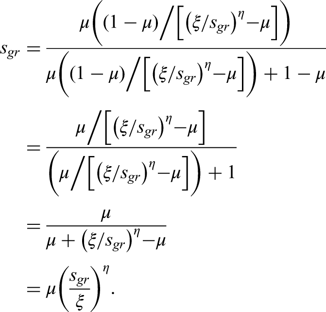
Let us assume in what follows that (5) does hold. Then, applying (59), the share of capital is

α (k) = \frac{k f^{'} (k)}{f (k)} = \frac{μ k^{η}}{μ k^{η} + 1 - μ} .

(62)

Note, as mentioned previously, that for the Cobb–Douglas case of

η = 0

the share of capital simplifies to the constant

μ

. In that instance, the Golden Rule savings rate that satisfies (27) is obviously

μ

too.

More generally, we have

\frac{d α (k)}{d k} = \frac{μ η k^{η - 1} (μ k^{η} + 1 - μ) - μ k^{η} (μ η k^{η - 1})}{(μ k^{η} + 1 - μ)^{2}} = \frac{(1 - μ) μ η k^{η - 1}}{(μ k^{η} + 1 - μ)^{2}},

(63)

so it is not quite so trivial to solve (27) for

s_{g r}

. Whether the share of capital increases or decreases with

k

depends on the sign of

η

. If

η > 0

, so capital and labor are substitutes, the share of capital will increase with

k

. If

η < 0

, so capital and labor are complements, the share will decrease with

k

Combining (62) and (57), we have

\begin{aligned} s_{g r} & = \frac{μ ((1 - μ) / [{(ξ / s_{g r})}^{η} - μ])}{μ ((1 - μ) / [{(ξ / s_{g r})}^{η} - μ]) + 1 - μ} \\ = \frac{μ / [{(ξ / s_{g r})}^{η} - μ]}{(μ / [{(ξ / s_{g r})}^{η} - μ]) + 1} \\ = \frac{μ}{μ + {(ξ / s_{g r})}^{η} - μ} \\ = μ {(\frac{s_{g r}}{ξ})}^{η} . \end{aligned}

Thus for CES production, the Golden Rule savings rate is

s_{g r} = {(\frac{μ}{ξ^{η}})}^{1 / (1 - η)} .

(64)

Using (56), we can also rewrite this as

s_{g r} = {(\frac{μ}{ξ^{η}})}^{σ} .

(65)

As we discussed above, the assumption (5) implies that

(ξ / μ^{1 / η}) ≷ 1

iff

η ≷ 0

, so

s_{g r} < 1

since

σ > 0

The elasticity of the share of capital is from (63)

\frac{k}{α (k)} \frac{d α (k)}{d k} = η \frac{1 - μ}{μ k^{η} + 1 - μ} = η (1 - α (k)) .

(66)

Then (41) gives

α_{2} (k) = \frac{k}{α (k)} \frac{d α (k)}{d k} - (1 - α (k)) = (η - 1) (1 - α (k)) < 0.

(67)

Thus we confirm via (42) that the elasticity of substitution is

1 / (1 - η)

. Applying (63) again:

\frac{d α_{2} (k)}{d k} = (1 - η) \frac{d α (k)}{d k} = (1 - η) \frac{(1 - μ) μ η k^{η - 1}}{(μ k^{η} + 1 - μ)^{2}} = (1 - η) η \frac{α (k) (1 - α (k))}{k} .

(68)

The corresponding elasticity is

\frac{k}{α_{2} (k)} \frac{d α_{2} (k)}{d k} = \frac{k}{(η - 1) (1 - α (k))} (1 - η) η \frac{α (k) (1 - α (k))}{k} = - η α (k) .

(69)

Finally, we use (41) once more to obtain the critical elasticity

α_{3} (k)

α_{3} (k) = \frac{k}{α_{2} (k)} \frac{d α_{2} (k)}{d k} - (1 - α_{2} (k)) = - η α (k) + (η - 1) (1 - α (k)) - 1

The aberrancy of a CES production function is

α_{3} (k) = η - 2 + (1 - 2 η) α (k),

(70)

which has an ambiguous sign.

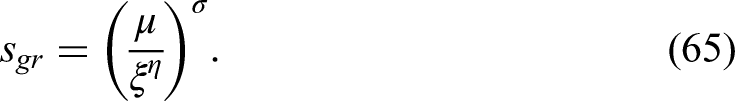
For the CES class of production functions, the dynamic inefficiency condition (50) is

η - 2 + (1 - 2 η) s_{g r} - 3 s_{g r} (1 - η - 2) < 0,

(71)

which simplifies to

(η + 4) s_{g r} < 2 - η .

(72)

Since

2 - η

is strictly positive, we can write this as a lower bound on the inverse Golden Rule savings rate:

\frac{1}{s_{g r}} > \frac{η + 4}{2 - η} .

(73)

Since

η = \frac{σ - 1}{σ},

we can also express the lower bound in terms of the elasticity of substitution:

\frac{1}{s_{g r}} > \frac{5 σ - 1}{σ + 1} .

(74)

For

σ \leq 0.2

, the lower bound is negative and obviously satisfied for any possible Golden Rule savings rate. For

σ > 0.2

, we can flip (74) to obtain

s_{g r} < \frac{σ + 1}{5 σ - 1} .

(75)

The right-hand side is a decreasing function of

σ

for

σ > 0.2

. Indeed, the bound only begins to bind for

σ > 0.5

. In the limit as capital and labor become perfect substitutes, dynamic inefficiency will still be optimal for

s_{g r} < 0.2

Recall that if $σ < 1$ (or $η <$ 0) then $c^{*} (s) = 0$ for $s \leq \underline{s}$ . Using (61) and (64), we have

\underline{s} = s_{g r}^{(η - 1) / η} = s_{g r}^{1 / (1 - σ)} < s_{g r} .

(76)

In the limit as

σ \to 1

\underline{s} \to 0

. However, as

σ

decreases from 1,

\underline{s}

gets larger, approaching

s_{g r}

, which in turn approaches

ξ < 1

, in the limit as capital and labor become perfect complements. When capital and labor become more complementary, capital becomes more essential to production, so the social planner cannot afford to gamble on the side of dynamic efficiency and possibly risk the collapse of the economy.

Since the numerator of (51) is (71), we get that the optimal ratio of the buffer to the noise variance for small $τ$ is

lim_{τ \to 0} \frac{Δ s}{τ^{2}} = - \frac{1}{2} \frac{η - 2 + (4 + η) s_{g r}}{(1 - s_{g r}) s_{g r}} .

(77)

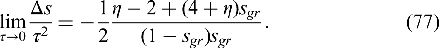
In Figure 1, we show how steady-state consumption varies with the savings rate for various choices of

η

with

μ = 0.33

and

ξ = 0.1

, which are both typical calibrations of

μ

and

ξ

for the United States when

η = 0

. For the Cobb–Douglas case of

η = 0

, steady-state consumption is maximized at

s = μ

. Since

μ < 0.5

, consumption falls off more quickly for lower savings rates than for higher savings rates, so the social planner would prefer a dynamically inefficient savings rate higher than the Golden Rule. As we make

η

negative, the Golden Rule savings rate, that is, the peak of the graph, decreases, and the falloff for

s < s_{g r}

becomes much steeper. This is in part because

c^{*} (s)

is only positive for

s > \underline{s}

and

\underline{s}

gets closer to

s_{g r}

η

decreases. Conversely, if we make

η

positive, then

s_{g r}

increases. For

η = 0.3

, the Golden Rule savings rate is 0.56. Since

s_{g r}

is closer to one than zero, the falloff is steeper to the right than to the left, so the social planner would prefer a dynamically efficient savings rate less than the Golden Rule.

Figure 1.

Graphs of steady-state consumption as a function of the savings rate $s$ for various choices of $η$ and with $μ = 0.33$ and $ξ = 0.1$ .

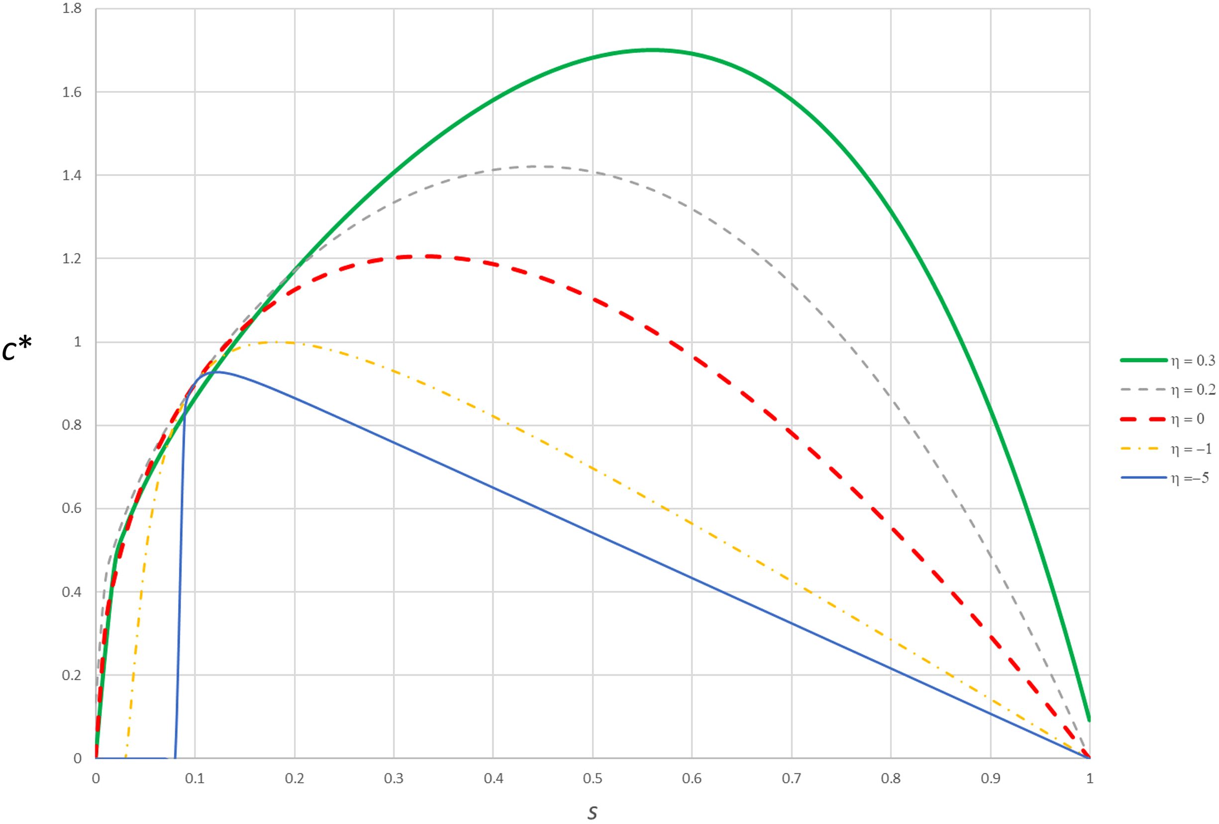
While the focus of the social planner is on steady-state consumption, it is useful to think about the implications of changing the savings rate on steady-state output as well. In Figure 2, we plot the corresponding graphs of steady-state output as a function of the savings rate. Note that while steady-state consumption is hump-shaped, the steady-state output is always strictly increasing if the output is positive, consistent with (24) since the output is a strictly increasing function of the capital stock. For $η = - 5$ , the graph is essentially flat for $s > s_{g r}$ . As we increase $η$ , the graph gets steeper.

Figure 2.

Graphs of steady-state output as a function of the savings rate $s$ for various choices of $η$ and with $μ = 0.33$ and $ξ = 0.1$ .

For the United States, $s$ is approximately 20 percent. For $η = 0$ , the Golden Rule savings rate is $s_{g r} = μ$ , that is, 33 percent. If we increase $s$ from 20 percent to 33 percent, $y^{*}$ changes from 1.4 to 1.8, which is an increase of 28%. In contrast, as is shown in Figure 1, $c^{*}$ only changes from 1.1 to 1.2, which is an increase of only 7%. If $η < 0$ ,²⁷ the gain in consumption from increasing the savings rate to the Golden Rule savings rate will be even smaller. Note that in the short run, consumption would have to decrease by another 10 percent from 1.1 to 1.0 (67% of 1.4) in order to make this change. The large short-run sacrifice and the small long-term gain help to explain why there is no impetus to make such a change in American politics today.

Application to China

In calibrating the model to China, we do not assume that China has already converged to a steady state. Instead, we assume China’s future macroeconomic history will be generated by (9) starting from the current capital per effective labor $k (0)$ with a fixed saving rate of $s = 0.433$ that is the average household savings rate between 2002 and 2020. Both Chen and Wen (2017) and Song, Storesletten, and Zilibotti (2011) use $n = 0.03$ per year, $δ = 0.1$ per year, and $g = 0.038$ per year. They also both set the income share of capital $α (k (0)) = 0.5$ , consistent with recent data.

We need the current capital–output ratio to pin down $k (0)$ . There is less agreement about this because researchers often estimate capital–output ratios separately for state-owned enterprises and domestic private enterprises. Song, Storesletten, and Zilibotti (2011) report ratios of 1.75 and 0.67, respectively, for these two types of enterprises. Since the state-owned enterprises dominate the Chinese economy, a value of 1.5 seems reasonable as an average $K / Y$ for the whole economy. Chen and Wen (2017), instead, report an average rate of profit of $r = 0.2$ . Given a share of the capital of 0.5 and a depreciation rate of 0.1, this implies $K / Y = 1.67$ . To accommodate the imprecision of these estimates, we consider two values, 1.5 and 1.75, that roughly contain these various estimates of $K / Y$ .

Since we do not have data with which to calibrate the elasticity of substitution between capital and labor, we proceed by considering different choices of $η$ , which relates to this elasticity via (56). Using (55), we can rewrite (62) as

α (k (0)) = μ {(\frac{K (0)}{Y (0)})}^{η}

(78)

since

K / Y = k / f (k)

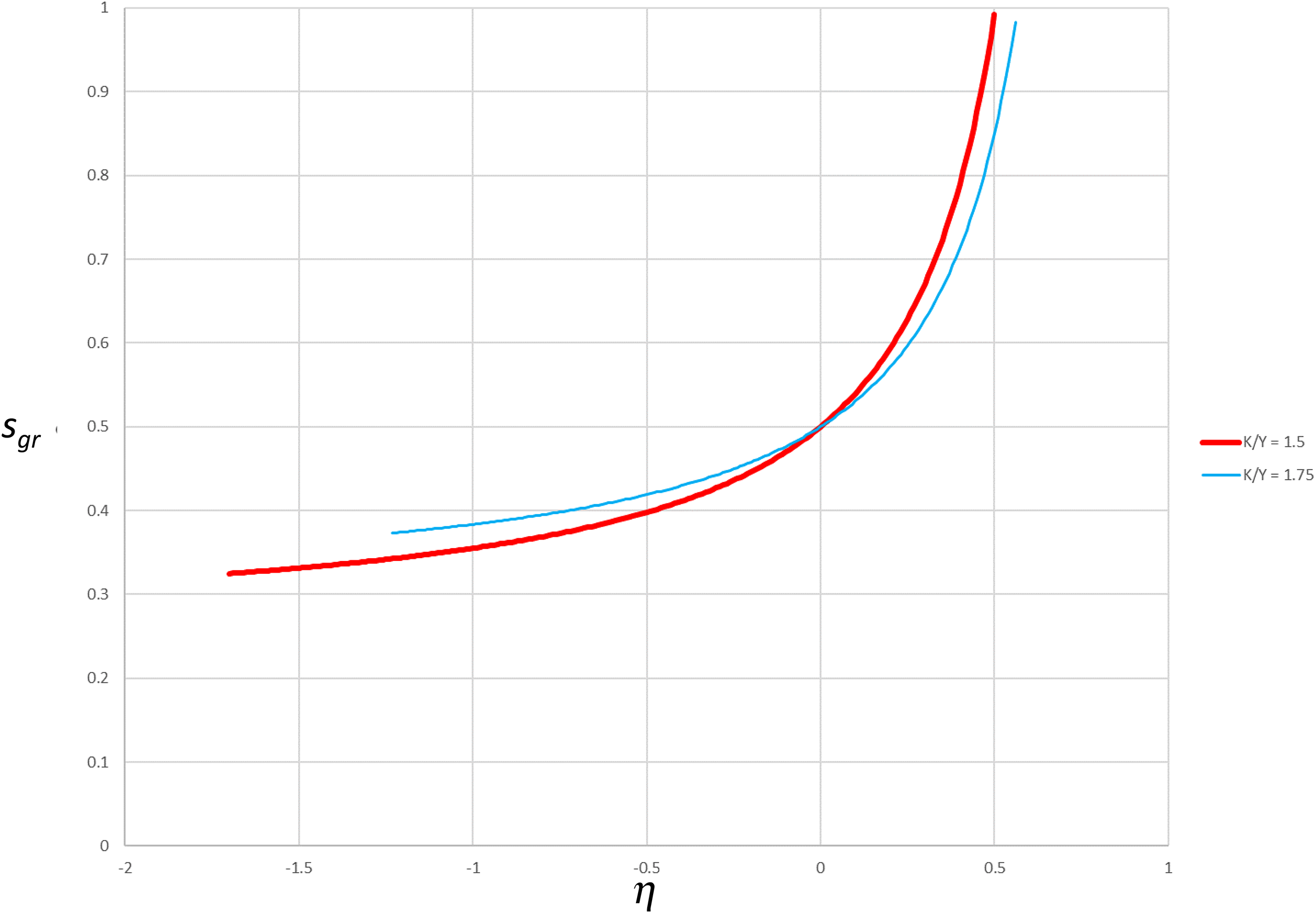
. This allows us to calibrate

μ

. Then we compute

s_{g r}

via (64), which we plot as a function of

η

for both choices of

K / Y

in Figure 3. We restrict attention to

η

such that

μ, s_{g r} \in (0, 1)

. Since

η > - 2

is necessary to satisfy both of these conditions, we always have

σ > 0.2

, so

\tilde{s} > s_{g r}

iff

s_{g r}

satisfies (74).

Figure 3.

Golden Rule savings rate as a function of $η$ for calibrations with $K / Y = 1.5$ or 1.75.

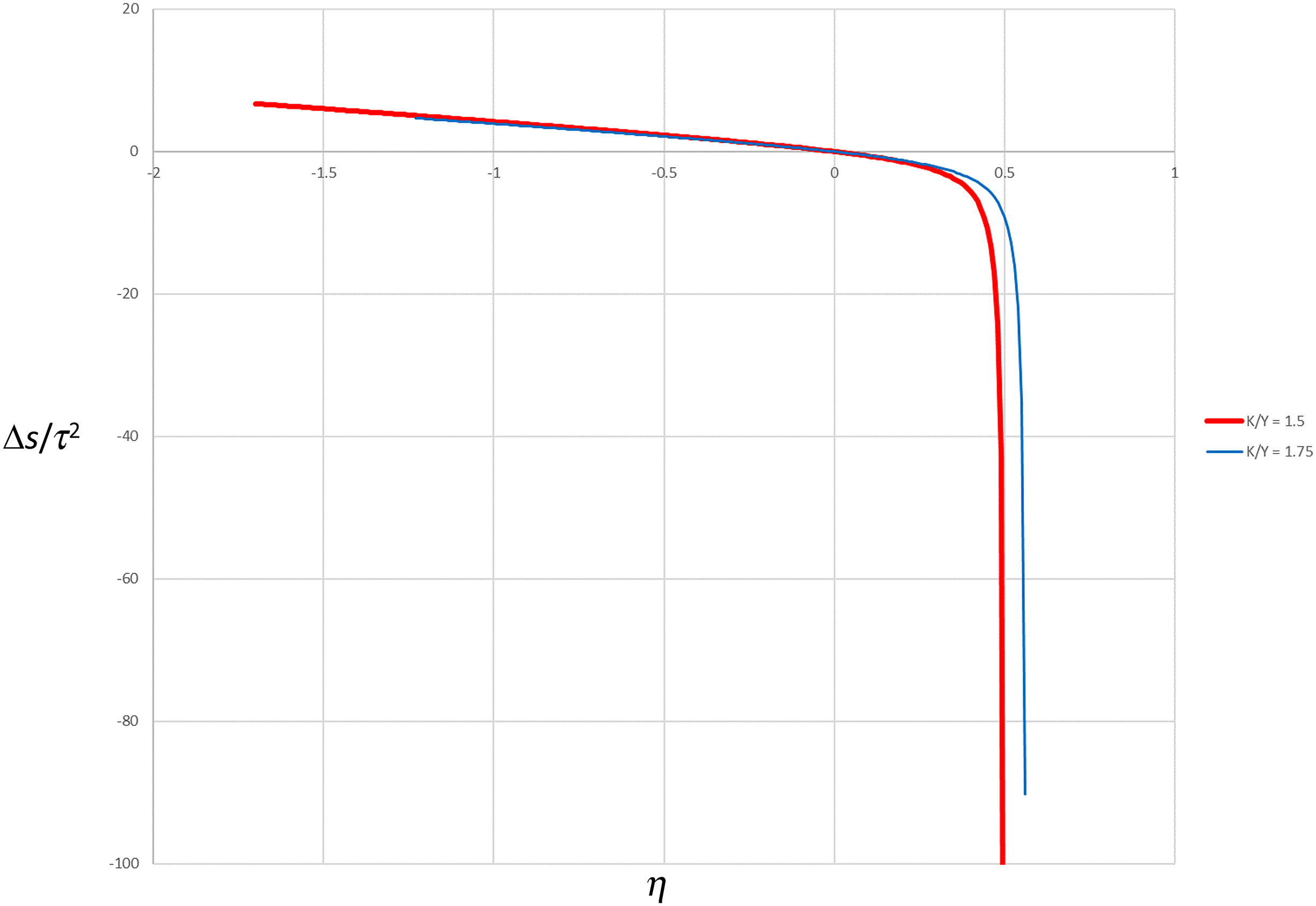
The optimal ratio of the buffer between the target savings rate and the Golden rule savings rate to the noise variance is plotted for the two choices of $K / Y$ in Figure 4. This ratio is strictly decreasing in $η$ and vanishes for $η = 0$ since, as we discussed in Section 4, steady-state consumption as a function of the savings rate is exactly symmetric around $s = 0.5$ if the production function is Cobb–Douglas and the share of capital is one-half. $η = 0$ is also the dividing point between where (74) is and is not satisfied. So dynamic inefficiency will be optimal for $η < 0$ . Thus the recent average savings rate of 43.3 percent could conceivably be optimal if $η$ (or $σ$ ) are low enough so that $s_{g r} < 0.433$ or if $η > 0$ . If $K / Y = 1.5$ , we would need either $σ < 0.788$ or $σ > 1$ . If $K / Y = 1.75$ , we would need either $σ < 0.726$ or $σ > 1$ .

Figure 4.

Ratio of optimal savings buffer to savings rate variance as a function of $η$ for calibrations with $K / Y = 1.5$ or 1.75.

As Figure 4 shows, the optimal buffer to variance ratio is less than ten in magnitude for almost the entire feasible parameter space of $η$ . If the standard deviation of $ε$ is on the order of a few percentage points, the variance of $ε$ will be on the order of $0.001$ , so the optimal buffer would typically be smaller than a percentage point.

We can discipline our calibration if we assume China is planning optimally and the variation in the observed savings rate in our sample is entirely due to variation in $ε$ , in which case we obtain $τ^{2} = 0.000683$ .²⁸ Though the optimal buffer to variance ratio gets very large in magnitude as $η$ approaches the upper limit where $s_{g r} \to 1$ , it does not get large enough to have $| Δ s | > 0.5$ . Thus the observed average savings rate can only be optimal if capital and labor are complementary. If $K / Y = 1.5$ , we need $σ = 0.788$ . If $K / Y = 1.75$ , we need $σ = 0.726$ . In both of these cases, the Golden Rule steady state is 43.2 percent, so dynamic inefficiency is optimal although the degree of inefficiency is quite small.

Concluding Remarks

We posit that it is an unnecessary stretch to model economies that are not associated with liberal democracies as standard neoclassical models featuring decentralized households that only coordinate their decisions via market-determined prices. Such economies can be described more parsimoniously with a Solow model that endogenizes the savings rate according to the principles of the governing regime. In the case of China, this approach can explain its high savings rate of 40 percent without any exotic assumptions about household preferences.

In a model with centralized decision-making, some of the most hallowed results from decentralized models need not carry over if the social planner does not have perfect control over the economy. We find that a social planner who wants to maximize long-run aggregate consumption ought not to balk at violating the neoclassical rule that you should never save more than the income share of capital. The concept of dynamic inefficiency only makes sense for a hypothetical social planner that is omnipotent. Real-world social planners are not so powerful. Unlike individual households, social planners will be held responsible for economywide disasters, so they have to hedge against them. If consumption is an asymmetric function of the realized savings rate in the vicinity of the Golden Rule savings rate that maximizes consumption, the social planner will want to adjust the savings rate in the direction such that the falloff in consumption is less steep. We establish a necessary and sufficient condition on the production function under which it is better to oversave. As capital and labor become less substitutable, dynamic inefficiency becomes optimal for a larger subset of the parameter space since saving becomes more essential to continue production. Calibrations of China that match recent savings data satisfy the condition for dynamic inefficiency to be optimal. Note that this result is not special to China. Given the shares of capital observed in cross-country data, if a social planner was to take over practically any existing economy, capital and labor would have to be extremely substitutable for dynamic efficiency to be socially optimal.

In this initial treatment of the subject of precautionary social planning, we are effectively assuming the social planner decides on a 1000-year plan. We model the choice of a permanent savings rate based on its effects on consumption in the long run. In future work, we will be studying how the social planner ought to modify the savings rate target during the transition to the steady state. This will be analogous to setting a sequence of five-year plans, as China does in practice.

Of course, the primary criticism of social planners is not that they do not accumulate enough capital but that they do not accumulate enough of the right kinds of capital. If we generalize the present model to allow for multiple types of capital and/or multiple consumption goods, we could look separately at the effects of the under-accumulation of capital versus the misallocation of capital. We are not aware of any serious attempt to quantify which of these errors is more costly. However, we may soon get empirical data on the costs of these different errors from the natural experiment of how well China competes with the West through the twenty-first century.

Footnotes

Acknowledgements

We would like to thank Nick Guo and Tom Rawski for many discussions and correspondence that culminated in this paper. We would also like to thank Erin Cottle Hunt, Ian King, Xianbai Li, Xueli Tang, Guillaume Vandenbroucke, and participants at the Midwest Macro Meeting for their comments and suggestions.

Declaration of Conflicting Interests

The author(s) declared no potential conflicts of interest with respect to the research, authorship, and/or publication of this article.

Funding

The author(s) received no financial support for the research, authorship, and/or publication of this article.

ORCID iD

James Feigenbaum

Notes

Author Biographies

Professor James Feigenbaum was born in Buffalo, New York and has a Ph.D. in economics from the University of Iowa and a Ph.D. in physics from the University of Chicago. He has worked as an intern and consultant at the Federal Reserve Bank of St. Louis and as an assistant professor at the University of Pittsburgh and now is a full professor in the Department of Economics and Finance at Utah State University. He is also an associate editor at Journal of Economic Dynamics and Control.

Tong Jin comes from Xi'an, China and has a master's degree in econometrics and quantitative economics from the University of Illinois Urbana-Champaign. He is a research assistant at Utah State University studying macroeconomics and comparative economics.

References

Cass

. 1965. “Optimal Growth in an Aggregative Model of Capital Accumulation.” Review of Economic Studies 32: 233–40.

Chen

Kaiji

Wen

. 2017. “The Great Housing Boom of China.” American Economic Journal: Macroeconomics 9 (2): 73–114.

Cukierman

Alex

. 2002. “Are Contemporary Central Banks Transparent About Economic Models and Objectives and What Difference Does It Make?” Federal Reserve Bank of St. Louis Review 84 (4): 15–35.

Diamond

Peter A

. 1965. “National Debt in a Neoclassical Growth Model.” American Economic Review 55: 1126–50.

Feigenbaum

James A

. 2019. “A Nonparametric Formula Relating the Elasticity of a Factor Demand to the Elasticity of Substitution.” Theoretical Economics Letters 9: 240–6.

Feigenbaum

James A.

Geng

. 2012. “Lifecycle Dynamics of Income Uncertainty and Consumption.” Advances in Macroeconomics 12 (1) Article 11.

Friedman

Milton

. 1953. Essays in Positive Economics. Chicago: University of Chicago Press.

Garriga

Carlos

Hedlund

Aaron

Tang

Yang

Wang

Ping

. 2021. “Rural–Urban Migration, Structural Transformation, and Housing Markets in China.” Utah Macro Workshop Presentation.

Guvenen

Fatih

. 2007. “Learning Your Earning: Are Labor Income Shocks Really Very Persistent?” American Economic Review 97: 687–712.

10.

Hui

Ning

Lei

Zhu

Dongming

. 2019. “The Impact of Rapid Aging and Pension Reform on Savings and the Labor Supply: The Case of China.” Working Paper.

11.

Koopmans

. 1965. “On the Concept of Optimal Growth.” In The Econometric Approach to Development Planning. Chicago: Rand-McNally.

12.

Leland

Hayne E

. 1968. “Saving and Uncertainty: The Precautionary Demand for Saving.” Quarterly Journal of Economics 82: 465–73.

13.

Marx

Karl

. 1875. “Critique of the Gotha Program,” https://www.marxists.org/archive/marx/works/download/Marx_Critque_of_the_Gotha_Programme.pdf.

14.

Ramsey

F.P

. 1928. “A Mathematical Theory of Saving.” Economic Journal 38: 543–59.

15.

Sandmo

. 1970. “The Effect of Uncertainty on Saving Decisions.” Review of Economic Studies 37: 353–60.

16.

Schot

Steven H

. 1978. “Geometry of the Third Derivative.” Mathematics Magazine 51 (5): 259–75.

17.

Solow

Robert M

. 1956. “A Contribution to the Theory of Economic Growth.” Quarterly Journal of Economics 70: 65–94.

18.

Song

Zheng

Storesletten

Kjetil

Zilibotti

Fabrizio

. 2011. “Growing Like China.” American Economic Review 101: 196–233.

19.

Wei

Shang-Jin

Zhang

Xiaobo

. 2011. “The Competitive Saving Motive: Evidence From Rising Sex Ratios and Savings Rates in China.” Journal of Political Economy 119: 511–64.