Political Budget Cycles in Latin America

Abstract

This study examines the relationship between elections and fiscal policies in Latin America during 2004–2019. We find that fiscal balance deteriorates and government expenditure increases during election years, confirming the existence of political budget cycles. Our generalized method of moments estimation suggests that governmental budget balance deteriorates between 0.6% and 0.8%, and government expenditure increases by 0.3%, during election years. Moreover, these political budget cycles are significantly larger in countries with high corruption levels than in those with low corruption levels. The difference can be explained by institutional factors. In our case, in countries with high corruption levels, possible rents for politicians are greater; hence, manipulating the fiscal tools before elections helps to maintain power.

Keywords

Political budget cycles elections public choice institutions

Introduction

Political budget cycles (PBCs) refer to the manipulation of fiscal policies during election years to enhance the likelihood of re-election. Incumbents’ behavior during those periods is an important concern in political economics because they may distort policymaking to serve their own interests (Mandon and Cazals 2019). The most common methods of manipulating fiscal policies include increasing expenditure (Petrakos et al. 2021), reducing tax rates (Alesina and Paradisi 2017), targeted spending (Eslava 2006), or clientelistic tools such as expanding public sector employment (Stolfi and Hallerberg 2016)

Various studies investigate the existence of PBCs, which represent the possibility of a macroeconomic cycle induced by a political cycle. Recent PBC models show that temporary asymmetries in politicians’ competencies influence electoral cycles (Gootjes, de Haan and Jong-A-Pin 2021). Therefore, the existence of PBCs helps explain how opportunistic incumbents manipulate economic policies to induce economic expansion before elections (Brender and Drazen 2005).

The existence of PBCs provide evidence that political actors act to please the electorate; hence, their policies concentrate more on political objectives, such as maintaining power, than on economic efficiency (López and Ignacio 2016). As such, social welfare is not the government's objective but a means to maximize its utility.

Fiscal tools are seemingly used to manipulate the economy and influence election results. Governments select policies that capture as many votes as possible, and expansionary fiscal policies help attract votes by allowing significant wealth transfers. These wealth transfers include cash transfers to households, employment and profit opportunities from public investment projects, tax rate reductions, and delayed tax collection (Schuknecht 2000). They can be implemented through expenditure or revenue; in either case, fiscal deficit is expected to increase before elections.

According to Mandon and Cazals (2019), since political-economic cycles are comparable to shocks affecting national budgets, they are likely to adversely affect economic growth and stability. Additionally, they state that public accounts that are manipulated because of elections reflect the imperfections of institutions and democracy.

The motivation behind incumbents’ decisions can be explained through public choice theory, which translates the hypothesis and methodologies from economics to the explanation and analysis of social phenomena in political sciences (Musgrave 1973). The theory considers the individuals studied in microeconomics as equivalent to politicians in the public sector in terms of motivation and behavior. Therefore, public choice theory assumes rationality. Rationality considers individuals capable of calculating and choosing results that determine their behavior and maximize their own utility; rational human beings are motivated to seek their own interests and make decisions coherently to achieve them (López and Ignacio 2016).

The influence of politicians on voters depends on the voter's information. PBCs are more prevalent where voters have limited information about the incumbent's performance or competence. Janků and Libich (2019) found that in countries with uninformed voters, politicians pretend to ‘buy’ votes by increasing public expenditure.

Voting decisions partly depend on voters’ rationality, preferences, and access to information. According to Wolfers (2002), completely rational voters should be able to differentiate signals from noise, that is, they should be able to differentiate indicators that show the real capacities of politicians from external factors that can be attributed erroneously. In reality, many voters choose governments because of economic fluctuations that do not result from their actions. Nevertheless, voting decisions involve considering the relative costs and benefits of obtaining and processing information. Therefore, rationality depends on whether voters efficiently use the available information to determine government competence.

Wolfers (2002) suggests a case in which voters interpret good economic results as evidence of politicians’ competence but do not differentiate signals from noise. In this scenario, politicians are encouraged to increase government expenditure before elections to convince the population that the good economic results are due to politicians’ competence. Therefore, the more voters fail to distinguish pre-electoral manipulations from incumbent competence, the more beneficial it is for incumbents to boost spending prior to elections (Shi and Svensson 2006). On the contrary, voters who are able to differentiate whether the good results are from the government's competence or a manipulation of government expenditure prior to elections penalize the party or incumbent by not voting for them. Either case depends on the personal preferences of voters, especially the availability and interest in obtaining information, considering the existing cost of access to information.

The incumbents’ incentives depend on the political-institutional environment. Specifically, they depend on the possible benefits from remaining in power, such as higher rent. This generates a greater incentive to manipulate fiscal rules before elections and influence voters’ decisions (Shi and Svensson 2006). Specifically, implementing expansionary policies before elections has significant incentives.

According to Alesina, Campante and Tabellini (2008), the lack of information and asymmetric information are important factors because voters observe the state of the economy, but not the rents that incumbents are taking as their own. Additionally, voters face corrupt governments that appropriate part of the revenue for unproductive consumption or to pay favors (political rent).

Politicians’ capacity to manipulate election results through fiscal policy and electorate voting decision is subject to political, economic, or legal restrictions. Each country's institutions depend on the political power of the groups and individuals who use the power for selfish interests. These political institutions determine the limits and incentives of other key actors in the political sphere and the distribution of political power, which affect economic institutions (Acemoglu, Johnson and Robinson 2015). Therefore, strengthening political institutions positively affects both economic institutions and the general economy.

The evidence is not robust to conclude that PBCs are a universal phenomenon; nevertheless, studies reveal their existence in less-developed countries, new or weak democracies, and parliamentary systems. Streb, Lema and Torrens (2009) find that cycles are statistically significant only in Latin America. Using data on Latin American countries from 1973 to 2008, Barberia and Avelino (2011) confirm that elections increase fiscal deficits due to increases in government expenditures.

PBC literature can be divided into two groups. The first focuses on determining whether PBC exists, specifically testing whether incumbents manipulate fiscal policy during election years. The second group centers on evaluating the effectiveness of the mechanism, which examines whether the incumbent wins the election or not. This study identifies the existence of PBCs in Latin America during 2004–2019. We assemble a panel dataset of 18 countries, and find evidence of PBCs. During election years, government global fiscal deficit, government primary fiscal deficit, and government expenditure increased have increased by 0.6%, 0.8%, and 0.65% of gross domestic product (GDP), respectively, while government revenues do not present significant results. We also find that countries with a high corruption index have stronger PBCs than countries with a low corruption index. The stronger PBCs are represented by greater government expenditure increases during election years.

The remainder of this paper is organized as follows. Section 2 presents previous studies on PBCs. Section 3 presents the dataset and econometric specifications. Section 4 presents the results of our analysis, which shows that PBCs exist in Latin America and they differ in magnitude depending on the corruption index. Section 5 identifies the different institutional factors that explain the existence of PBCs and discuss possible future investigations. Section 6 includes robustness tests, and Section 7 concludes the study.

Literature Review

Mandon and Cazals (2019) suggest that cycles are more likely to occur for instruments such as fiscal policy rather than for economic policy outcomes, such as unemployment, growth, or inflation. Furthermore, in political business cycles, voters presumably choose leaders based on economic variables; therefore, the “degree, nature and timing of economic policies influence citizens’ decision at the ballot box” (Barberia and Avelino 2011).

Although PBCs are extensively studied, their appearance is heterogeneous and conditional. They are examined based on different factors, such as the development level, quality of institutions, characteristics of democracy, and constitutional features (Mandon and Cazals 2019). Some studies indicate that PBCs are more prevalent in developing countries (Schuknecht 2000; Shi and Svensson 2006), low-level democratic regimes (Gonzalez 2002), and new democracies (Brender and Drazen 2005). One possible explanation for this phenomenon is that voters in these countries are usually less informed and experienced; thus, government manipulation is expected to be more effective.

Corruption frequently correlates with rising public spending that incumbents may exploit for electoral gain (Aktaş 2021; Moschovis 2010; Sironi and Tornari 2013). Nguyen and Tran (2023) found that PBC occurs in emerging and developing countries. In these countries, incumbents tend to raise government spending before elections and subsequently cut it afterward. This study indicates that enhancing corruption control can mitigate the impact of PBCs.

Schuknecht (2000) examines 24 developing countries for the period 1973–1992 and finds an increase in public expenditure during pre-electoral periods; two-thirds of the increase in fiscal deficits of approximately 0.7% of GDP around elections is due to an increase in public expenditure. Shi and Svensson (2006), through a panel data of a set of 85 countries over the period 1975–1995 find evidence of PBCs and reveal that, on average, government fiscal deficit increases by almost 1% of GDP in election years. Moreover, these political budget cycles are significantly larger and statistically more robust in developing countries than in developed countries (Shi and Svensson 2006). Streb, Lema and Torrens (2009) compare the existence of PBCs in Latin American and OECD countries and find that cycles are statistically significant only in Latin America.

Mandon and Cazals (2019), through a meta-analysis, conclude that fiscal balance systematically deteriorates before elections; although, these conclusions should be taken with caution due to the possible exaggeration of results by researchers. They also indicate that recent studies have found that the magnitude of PBCs have declined due to better estimates. However, most studies indicate that the quality of political institutions is the most influential factor in the existence of PBCs.

Latin America has experienced widespread instability and macroeconomic fluctuation in recent decades. Consequently, most of the literature on PBCs focuses on this region.¹ Ames (1987) finds that in 17 Latin American countries, between 1947 and 1982, government expenditures have increased by 6.3% in the year before and have decreased by 7.6% in the year after elections.

Other studies focus on a subset of Latin American countries. In their study of 8 Latin American countries, Mejía-Acosta and Coppedge (2001) find that during 1979–1998, the budget deficit worsens during elections; although, the higher budget deficit is not due to government expenditure.

This study uses data from 18 Latin American countries for the period 2004–2019 to clarify the existence of PBCs. We examine whether PBCs come from an increase in government expenditure or a decrease in government revenues and analyze them by differentiating between global fiscal balance and primary fiscal balance. Furthermore, we classify countries using a corruption index to find evidence based on institutional factors.

Method

We present the model to test the effect of elections on fiscal variables that takes the following empirical specifications:

Y_{i, t} = \sum_{j = 1}^{2} γ_{j} Y_{i, t - j} + η Z_{i, t} + β E L E_{i, t} + c_{i} + ε_{i, t}

(1)

This is a dynamic panel model in which the dependent variable is a function of its own lagged levels and a set of independent variables. We use Brender and Drazen's (2005) three measures of fiscal policy: total government spending, total revenue collection, and budget balance (global and primary)—all as a share of GDP. Z is a vector of the control variables. The index i refers to the N observational units (country) and t is year. $E L E_{i, t}$ is an election dummy variable, $c_{i}$ is an unobserved country-specific effect, and $ε_{i, t}$ is an i.i.d. error term. In all regressions, we include the logarithm of real GDP per capita and GDP growth rate as control variables to capture the effects of the business cycle on budget surplus, government expenditure, and government revenue.

The inclusion of lagged dependent variables and the existence of country-specific effects cause the ordinary least squares estimator to be biased. Therefore, we follow Shi and Svensson (2006) and use fixed-effects (FE) estimators² to eliminate country-specific effects, and make the results comparable with more studies. However, FE does not eliminate the bias caused by the inclusion of lagged dependent variables. As established by Shi and Svensson (2006), the bias of the FE estimator, “depends on the length of the time series and only when it goes to infinity will the FE estimator be consistent” (2006). Our sample has 16 observations across countries, which cause the FE estimator to be biased.

We use the generalized method of moments (GMM) estimator by Arellano and Bond (1991), Arellano and Bover (1995), and Blundell and Bond (1998) to solve the problem. The GMM estimator controls for unobserved country-specific effects and bias caused by lagged dependent variables. The model does not control for time effects because it controls for seasonality and the data used are annual. We use the period 2004–2019, considering that for the GMM estimation, we use only the years 2004–2020, because the model requires a small T (number of periods compared to N (number of countries) (T > N).

The data, except for the election year, is obtained from the World Economic Outlook (WEO) database published by the International Monetary Fund. The data belong to the general government and are as a share of GDP: global net lending/borrowing (BUDGETG), primary net lending/borrowing (BUDGETP), total government expenditure (EXPENDITURE), and government revenue (REVENUE). Percentage changes in GDP (Growth) and GDP per capita (GDPpp) data are also obtained from the WEO.

General government consists of the central government, state government, local government, and social security funds. The general government fiscal balance (net lending (+) or net borrowing (-) of the general government) is total general government revenue minus total general government expenditure. Revenue includes social contributions, taxes other than social contributions, and grants. Conversely, expenditure includes intermediate consumption, employee compensation, subsidies, social benefits, other current expenditure (including interest spending), capital transfers, and other capital expenditure. Unlike the global fiscal balance, primary fiscal balance does not include interest payments. Gootjes, de Haan and Jong-A-Pin (2021) do not consider primary fiscal balance because interest payments “do not reflect fiscal policies in the current period”. Nevertheless, we include it for comparison purposes.

The key independent variable is the binary election variable, the electoral year dummy (ELECTION), which is equal to one in the election year and zero otherwise. We consider only country-wide general presidential elections. The election year is selected based on the rule of the semester. If an election is held during the first half of year t, then the election year is coded as the year before or t – 1; if the election is held during the second half of year t, the election year is coded as the same year (Barberia and Avelino 2011). This is because expansionary policies are expected to start during the fiscal year preceding the election if the ballot happens during the first semester. Electoral calendar of each country is obtained from various sources.

As previously mentioned, institutional factors significantly influence the existence of PBCs. Despite the difficulty in measuring politicians’ rents, we follow Shi and Svensson (2006) and use the corruption perception index from Transparency International as a proxy for politicians’ rents. The index is based on the degree of corruption as seen by business people and risk analysts. The index ranks 180 countries worldwide based on their perceived levels of public sector corruption, such as bribery, diversion of public funds, use of public functions for personal gain, nepotism in public administration, and capture of the state. We rescale the original index by calculating the average world ranking of each country from 2004 to 2019. Furthermore, we divide the countries in two groups: “low corruption” which includes countries that have an average CPI below the median, and “high corruption” which includes countries that have an average CPI above the median. We classify a third group which excludes Chile, Costa Rica, and Uruguay. They are excluded because they have an average CPI below 50, which is more than the standard deviation below the group average. As a robustness test, we have used the Worldwide Governance Indicators from the World Bank (2024) to check whether our classification (i) high corruption and (ii) low corruption remains equal. We found that the classification is exactly the same using CPI from Transparency International and the Control of Corruption from the World Bank. Cooray and Özmen (2024) argue that the control of corruption and the CPI are proxies of strong institutions that promote the better use of fiscal frameworks.

We have also checked if our classification remains the same using other governance and institutional indicators such as governance effectiveness, political stability, regulatory quality, rule of law, and voice and accountability. We conclude that the classification has a subtle shift in most cases. Therefore, we maintain the initial classification. Table 1 shows the comparison between CPI vs. Control of Corruption and other institutional indicators.

Table 1.

Corruption Indicators and World Governance Indicators.

Country	Corruption Perception Index	Control of Corruption	Government Effectiveness	Political Stability	Regulatory Quality	Rule of Law	Voice and Accountability	Number of Elections 2004–2019
Argentina	Low	Low	Low	Low	High	Low	Low	4
Bolivia	High	High	High	High	High	High	High	4
Brazil	Low	Low	Low	Low	Low	Low	Low	4
Chile	Low	Low	Low	Low	Low	Low	Low	4
Colombia	Low	Low	Low	High	Low	Low	High	4
Costa Rica	Low	Low	Low	Low	Low	Low	Low	4
Ecuador	High	High	High	High	High	High	High	4
El Salvador	Low	Low	Low	Low	Low	High	High	3
Guatemala	High	High	High	High	High	High	High	4
Honduras	High	High	High	High	High	High	High	4
Mexico	High	High	Low	High	Low	Low	Low	3
Nicaragua	High	High	High	Low	High	High	High	3
Panama	Low	Low	Low	Low	Low	Low	Low	3
Paraguay	High	High	High	High	High	High	High	3
Peru	Low	Low	High	High	Low	Low	Low	3
Dom. Republic	High	High	High	Low	High	High	Low	3
Uruguay	Low	Low	Low	Low	Low	Low	Low	4
Venezuela	High	High	High	High	High	High	High	3

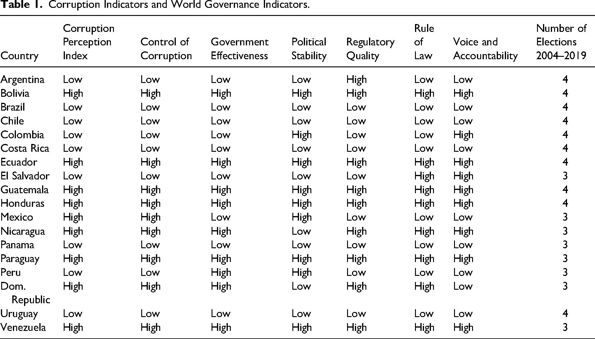
Previous evidence has shown that the control of corruption is correlated with other governance and institutional indicators, such as regulatory quality, political stability, and voice and accountability (Chong, Tee and Cheng 2020; Destek et al. 2023; Kwakwa and Aboagye 2024). These elements together enhance governance and diminish corruption (Udemba, Onyenegecha and Olasehinde‐Williams 2022).

Table 1 also provides an overview of the sample countries, the number of elections that have taken place during the sample period. Our final sample consists of 18 countries and 288 observations. On average, 3.5 elections are held in each country during the sample period, translating to roughly one election every fourth year.

Table 2 presents descriptive statistics for the key variables. The average global fiscal balance for the sample period is 2.54% of GDP, that is, a global deficit of fewer than 3% of GDP with a standard deviation of 3.57. The primary fiscal balance is −0.44% of GDP with a standard deviation of 3.62. The government expenditure and revenue are 25.8% and 23.2% of GDP, respectively.

Table 2.

Descriptive Statistics of key Variables.

Variable	Sample	Mean	Std. dev.	No. obs.	No. countries
Global Fiscal balance/GDP	All	−2.56	3.57	378	18
	Low corruption	−2.56	2.91	189	9
	High corruption	−2.54	4.13	189	9
	URY, CHL, CRI	−1.95	3.26	51	3
Primary Fiscal balance/GDP	All	−0.44	3.62	378	18
	Low corruption	−0.24	2.64	189	9
	High corruption	−0.91	4.35	189	9
	URY, CHL, CRI	0.09	2.92	51	3
Government expenditure/GDP	All	25.79	7.75	378	18
	Low corruption	25.4	7.63	189	9
	High corruption	26.18	7.85	189	9
	URY, CHL, CRI	23.26	4.84	51	3
Government revenue/GDP	All	23.23	7.01	378	18
	Low corruption	22.99	6.93	189	9
	High corruption	23.47	7.1	189	9
	URY, CHL, CRI	21.31	5.69	51	3
Corruption Index (CPI)	All	100	38.54	378	18
	Low corruption	71.01	30.04	189	9
	High corruption	130.88	16.67	189	9
	URY, CHL, CRI	30	10	51	3

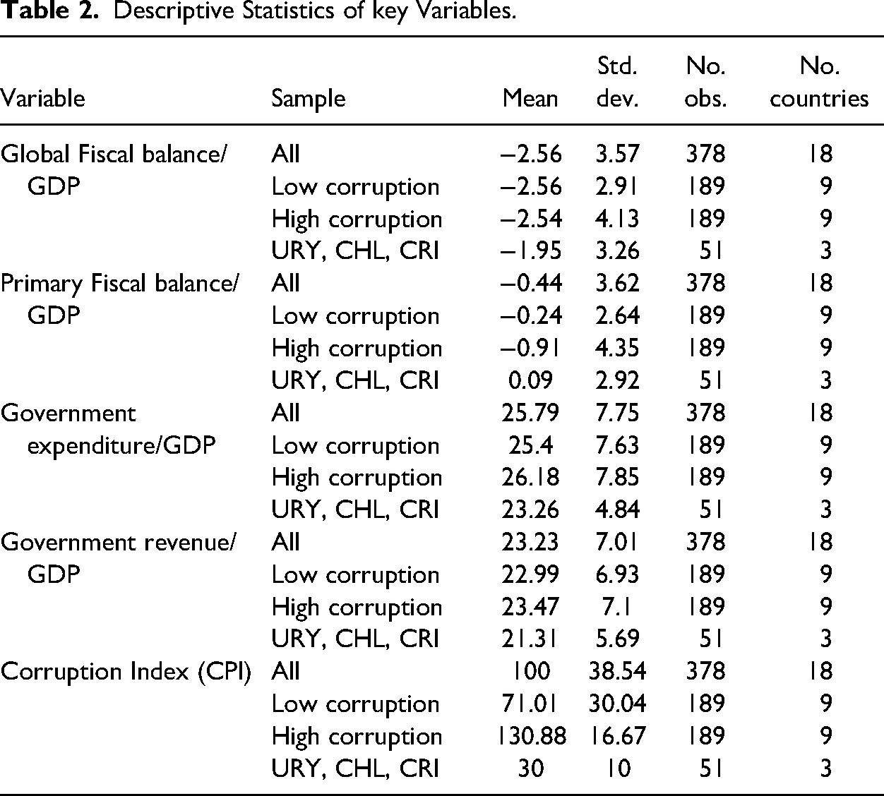
Looking at the raw cross-country data, the average CPI score differs significantly between the two subsamples. The average rank in the 18 countries is 100, while the average rank with low corruption is 71, and that with high corruption is 130.9.

Table 2 also includes data for Uruguay, Chile, and Costa Rica, the three countries that are excluded in the third group estimation. The measures for all key variables are much lower for the three countries.

Our final sample has all the data on general government fiscal budget balance, expenditure, revenue, elections, GDP growth rate, and GDP per capita; therefore, we have a completely balanced panel.

Results

We present the results for the four dependent variables. All regressions include two lagged values of the dependent variable, two control variables (logarithm of real GDP per capita and growth rates), and an election indicator, as established by Brender and Drazen (2005).

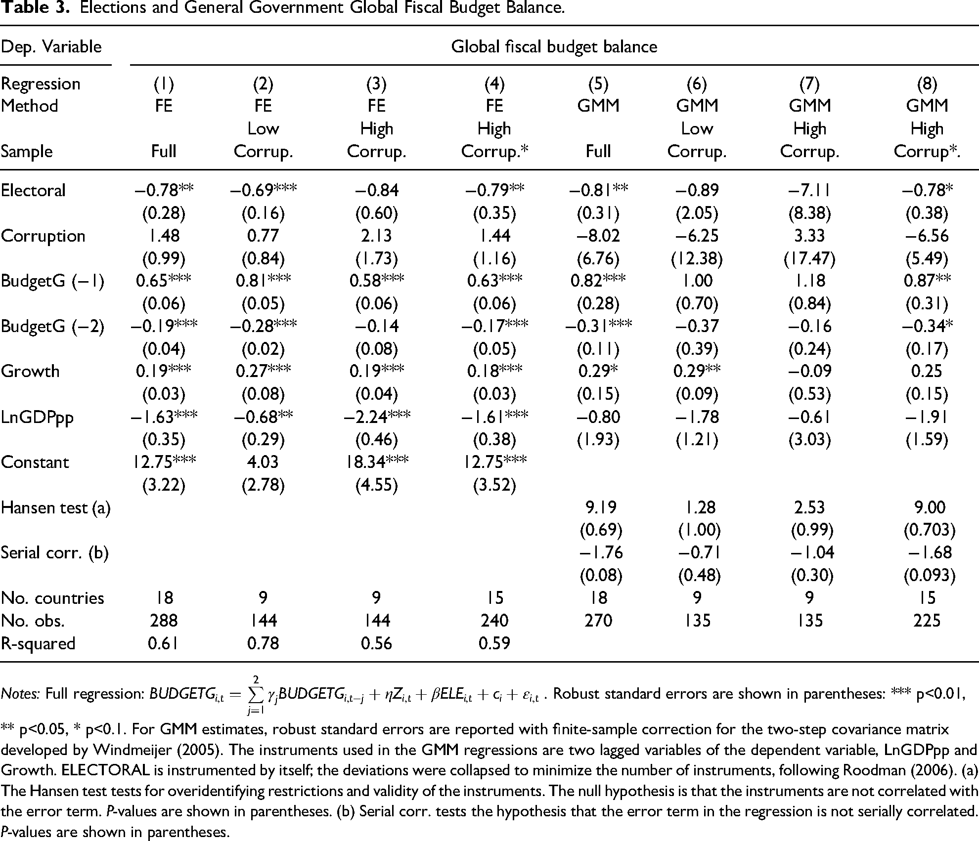
Table 3 reports the baseline findings for global fiscal balance. Columns 1–4 present the results of the FE estimation.³ The coefficient of ELECTORAL suggests a negative relationship between elections and global fiscal balance. The results in Column 1 indicate that in Latin America, the global fiscal deficit as a share of GDP is 0.78 percentage points higher in election years.

Table 3.

Elections and General Government Global Fiscal Budget Balance.

Dep. Variable	Global fiscal budget balance
Regression	(1)	(2)	(3)	(4)	(5)	(6)	(7)	(8)
Method	FE	FE	FE	FE	GMM	GMM	GMM	GMM
Sample	Full	Low Corrup.	High Corrup.	High Corrup.*	Full	Low Corrup.	High Corrup.	High Corrup*.
Electoral	−0.78**	−0.69***	−0.84	−0.79**	−0.81**	−0.89	−7.11	−0.78*
	(0.28)	(0.16)	(0.60)	(0.35)	(0.31)	(2.05)	(8.38)	(0.38)
Corruption	1.48	0.77	2.13	1.44	−8.02	−6.25	3.33	−6.56
	(0.99)	(0.84)	(1.73)	(1.16)	(6.76)	(12.38)	(17.47)	(5.49)
BudgetG (−1)	0.65***	0.81***	0.58***	0.63***	0.82***	1.00	1.18	0.87**
	(0.06)	(0.05)	(0.06)	(0.06)	(0.28)	(0.70)	(0.84)	(0.31)
BudgetG (−2)	−0.19***	−0.28***	−0.14	−0.17***	−0.31***	−0.37	−0.16	−0.34*
	(0.04)	(0.02)	(0.08)	(0.05)	(0.11)	(0.39)	(0.24)	(0.17)
Growth	0.19***	0.27***	0.19***	0.18***	0.29*	0.29**	−0.09	0.25
	(0.03)	(0.08)	(0.04)	(0.03)	(0.15)	(0.09)	(0.53)	(0.15)
LnGDPpp	−1.63***	−0.68**	−2.24***	−1.61***	−0.80	−1.78	−0.61	−1.91
	(0.35)	(0.29)	(0.46)	(0.38)	(1.93)	(1.21)	(3.03)	(1.59)
Constant	12.75***	4.03	18.34***	12.75***
	(3.22)	(2.78)	(4.55)	(3.52)
Hansen test (a)					9.19	1.28	2.53	9.00
					(0.69)	(1.00)	(0.99)	(0.703)
Serial corr. (b)					−1.76	−0.71	−1.04	−1.68
					(0.08)	(0.48)	(0.30)	(0.093)
No. countries	18	9	9	15	18	9	9	15
No. obs.	288	144	144	240	270	135	135	225
R-squared	0.61	0.78	0.56	0.59

Notes: Full regression: $B U D G E T G_{i, t} = \sum_{j = 1}^{2} γ_{j} B U D G E T G_{i, t - j} + η Z_{i, t} + β E L E_{i, t} + c_{i} + ε_{i, t}$ . Robust standard errors are shown in parentheses: *** p<0.01, ** p<0.05, * p<0.1. For GMM estimates, robust standard errors are reported with finite-sample correction for the two-step covariance matrix developed by Windmeijer (2005). The instruments used in the GMM regressions are two lagged variables of the dependent variable, LnGDPpp and Growth. ELECTORAL is instrumented by itself; the deviations were collapsed to minimize the number of instruments, following Roodman (2006). (a) The Hansen test tests for overidentifying restrictions and validity of the instruments. The null hypothesis is that the instruments are not correlated with the error term. P-values are shown in parentheses. (b) Serial corr. tests the hypothesis that the error term in the regression is not serially correlated. P-values are shown in parentheses.

This percentage is higher for countries with a high corruption (Column 3), as global fiscal deficit as share of GDP increases by 0.84 percentage points in election years. For countries with a low corruption (Column 2), the global fiscal deficit increases as the share of GDP increases by 0.69 percentage points in election years. We also calculate for the third group (Column 4), and the result shows that the group's global fiscal deficit as a share of GDP is 0.79 percentage points higher in election years.

Columns 5–8 present the results of the GMM estimation. Only the results for the full sample are significant,⁴ which confirms the existence of PBCs in Latin America, but in a lower dimension. The results show that during election years, the global fiscal deficit increases by 0.81 percent of GDP.

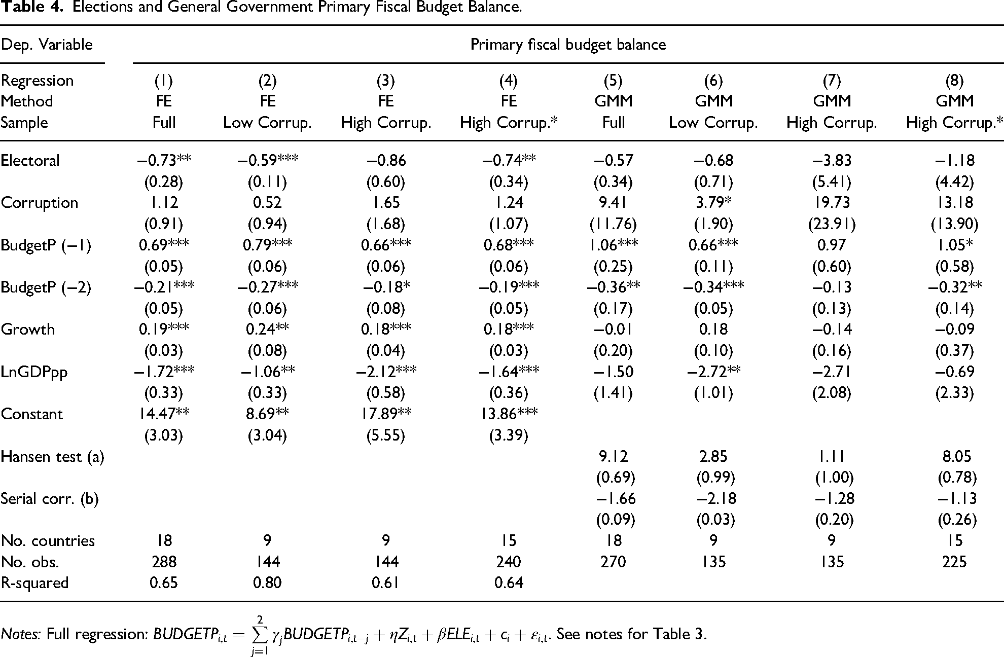
Table 4 reports the baseline findings of primary fiscal balance. Primary fiscal balance, unlike global fiscal balance, does not consider interest payments. Thus, primary fiscal deficit is lower than global fiscal deficit. As in Table 3, columns 1–4 report the FE estimation results, while columns 5–8 present the GMM estimation results. The negative coefficient on ELECTORAL suggests a negative relationship between elections and primary fiscal balance. The results for the full sample presented in column 1 indicate that in election years, primary fiscal deficit increases by 0.73 percent of GDP, similar to the results for global fiscal deficit. The results for the high corruption group and the third group are similar to those for global fiscal deficit. Column 2 presents the results for the low corruption group, which show that primary fiscal deficit is higher by (0.59) percentage points of GDP.

Table 4.

Elections and General Government Primary Fiscal Budget Balance.

Dep. Variable	Primary fiscal budget balance
Regression	(1)	(2)	(3)	(4)	(5)	(6)	(7)	(8)
Method	FE	FE	FE	FE	GMM	GMM	GMM	GMM
Sample	Full	Low Corrup.	High Corrup.	High Corrup.*	Full	Low Corrup.	High Corrup.	High Corrup.*
Electoral	−0.73**	−0.59***	−0.86	−0.74**	−0.57	−0.68	−3.83	−1.18
	(0.28)	(0.11)	(0.60)	(0.34)	(0.34)	(0.71)	(5.41)	(4.42)
Corruption	1.12	0.52	1.65	1.24	9.41	3.79*	19.73	13.18
	(0.91)	(0.94)	(1.68)	(1.07)	(11.76)	(1.90)	(23.91)	(13.90)
BudgetP (−1)	0.69***	0.79***	0.66***	0.68***	1.06***	0.66***	0.97	1.05*
	(0.05)	(0.06)	(0.06)	(0.06)	(0.25)	(0.11)	(0.60)	(0.58)
BudgetP (−2)	−0.21***	−0.27***	−0.18*	−0.19***	−0.36**	−0.34***	−0.13	−0.32**
	(0.05)	(0.06)	(0.08)	(0.05)	(0.17)	(0.05)	(0.13)	(0.14)
Growth	0.19***	0.24**	0.18***	0.18***	−0.01	0.18	−0.14	−0.09
	(0.03)	(0.08)	(0.04)	(0.03)	(0.20)	(0.10)	(0.16)	(0.37)
LnGDPpp	−1.72***	−1.06**	−2.12***	−1.64***	−1.50	−2.72**	−2.71	−0.69
	(0.33)	(0.33)	(0.58)	(0.36)	(1.41)	(1.01)	(2.08)	(2.33)
Constant	14.47**	8.69**	17.89**	13.86***
	(3.03)	(3.04)	(5.55)	(3.39)
Hansen test (a)					9.12	2.85	1.11	8.05
					(0.69)	(0.99)	(1.00)	(0.78)
Serial corr. (b)					−1.66	−2.18	−1.28	−1.13
					(0.09)	(0.03)	(0.20)	(0.26)
No. countries	18	9	9	15	18	9	9	15
No. obs.	288	144	144	240	270	135	135	225
R-squared	0.65	0.80	0.61	0.64

Notes: Full regression: $B U D G E T P_{i, t} = \sum_{j = 1}^{2} γ_{j} B U D G E T P_{i, t - j} + η Z_{i, t} + β E L E_{i, t} + c_{i} + ε_{i, t}$ . See notes for Table 3.

However, the results of the GMM estimation differ. For the primary fiscal balance, the deficit increases as a share of GDP in election years by 0.57 percentage points, which indicates a stronger political budget cycle when interest payments are not considered.

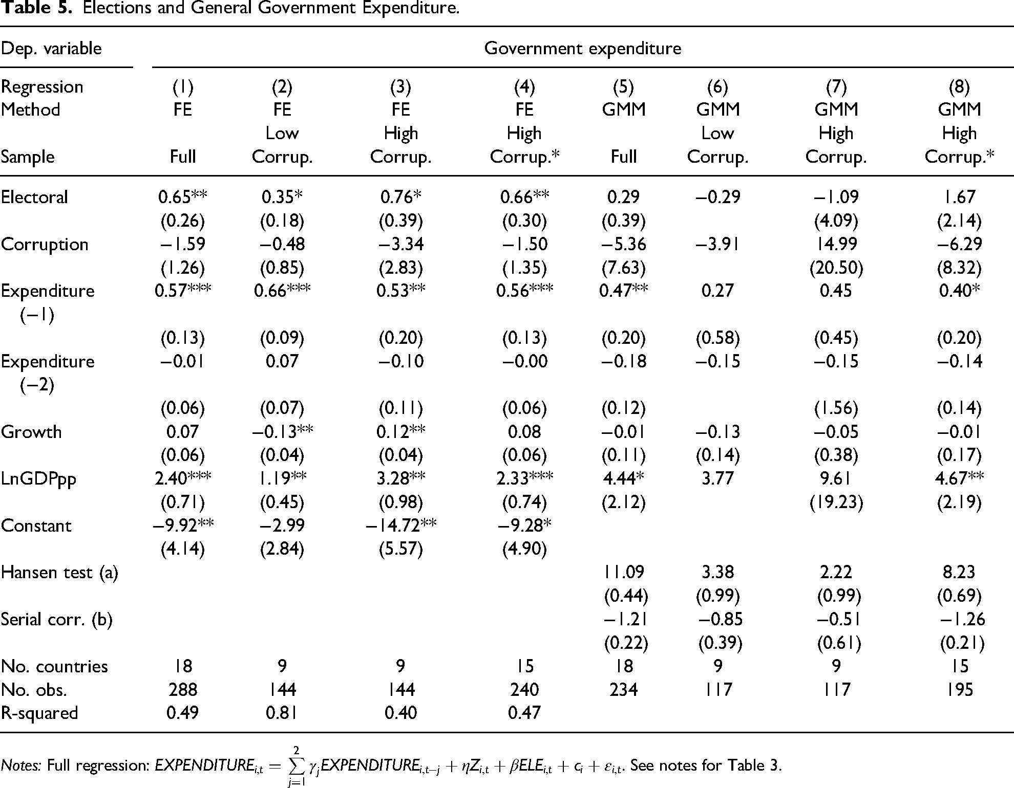
Table 5 presents the estimation results for expenditure. The results reveal a positive relationship between elections and expenditure, that is, in election years, general government expenditure increases. However, the results are only significant for the FE estimation for the full sample, and the third group that excludes Uruguay, Chile, and Costa Rica. Therefore, government expenditure increase in election year is higher in the third group.

Table 5.

Elections and General Government Expenditure.

Dep. variable	Government expenditure
Regression	(1)	(2)	(3)	(4)	(5)	(6)	(7)	(8)
Method	FE	FE	FE	FE	GMM	GMM	GMM	GMM
Sample	Full	Low Corrup.	High Corrup.	High Corrup.*	Full	Low Corrup.	High Corrup.	High Corrup.*
Electoral	0.65**	0.35*	0.76*	0.66**	0.29	−0.29	−1.09	1.67
	(0.26)	(0.18)	(0.39)	(0.30)	(0.39)		(4.09)	(2.14)
Corruption	−1.59	−0.48	−3.34	−1.50	−5.36	−3.91	14.99	−6.29
	(1.26)	(0.85)	(2.83)	(1.35)	(7.63)		(20.50)	(8.32)
Expenditure (−1)	0.57***	0.66***	0.53**	0.56***	0.47**	0.27	0.45	0.40*
	(0.13)	(0.09)	(0.20)	(0.13)	(0.20)	(0.58)	(0.45)	(0.20)
Expenditure (−2)	−0.01	0.07	−0.10	−0.00	−0.18	−0.15	−0.15	−0.14
	(0.06)	(0.07)	(0.11)	(0.06)	(0.12)		(1.56)	(0.14)
Growth	0.07	−0.13**	0.12**	0.08	−0.01	−0.13	−0.05	−0.01
	(0.06)	(0.04)	(0.04)	(0.06)	(0.11)	(0.14)	(0.38)	(0.17)
LnGDPpp	2.40***	1.19**	3.28**	2.33***	4.44*	3.77	9.61	4.67**
	(0.71)	(0.45)	(0.98)	(0.74)	(2.12)		(19.23)	(2.19)
Constant	−9.92**	−2.99	−14.72**	−9.28*
	(4.14)	(2.84)	(5.57)	(4.90)
Hansen test (a)					11.09	3.38	2.22	8.23
					(0.44)	(0.99)	(0.99)	(0.69)
Serial corr. (b)					−1.21	−0.85	−0.51	−1.26
					(0.22)	(0.39)	(0.61)	(0.21)
No. countries	18	9	9	15	18	9	9	15
No. obs.	288	144	144	240	234	117	117	195
R-squared	0.49	0.81	0.40	0.47

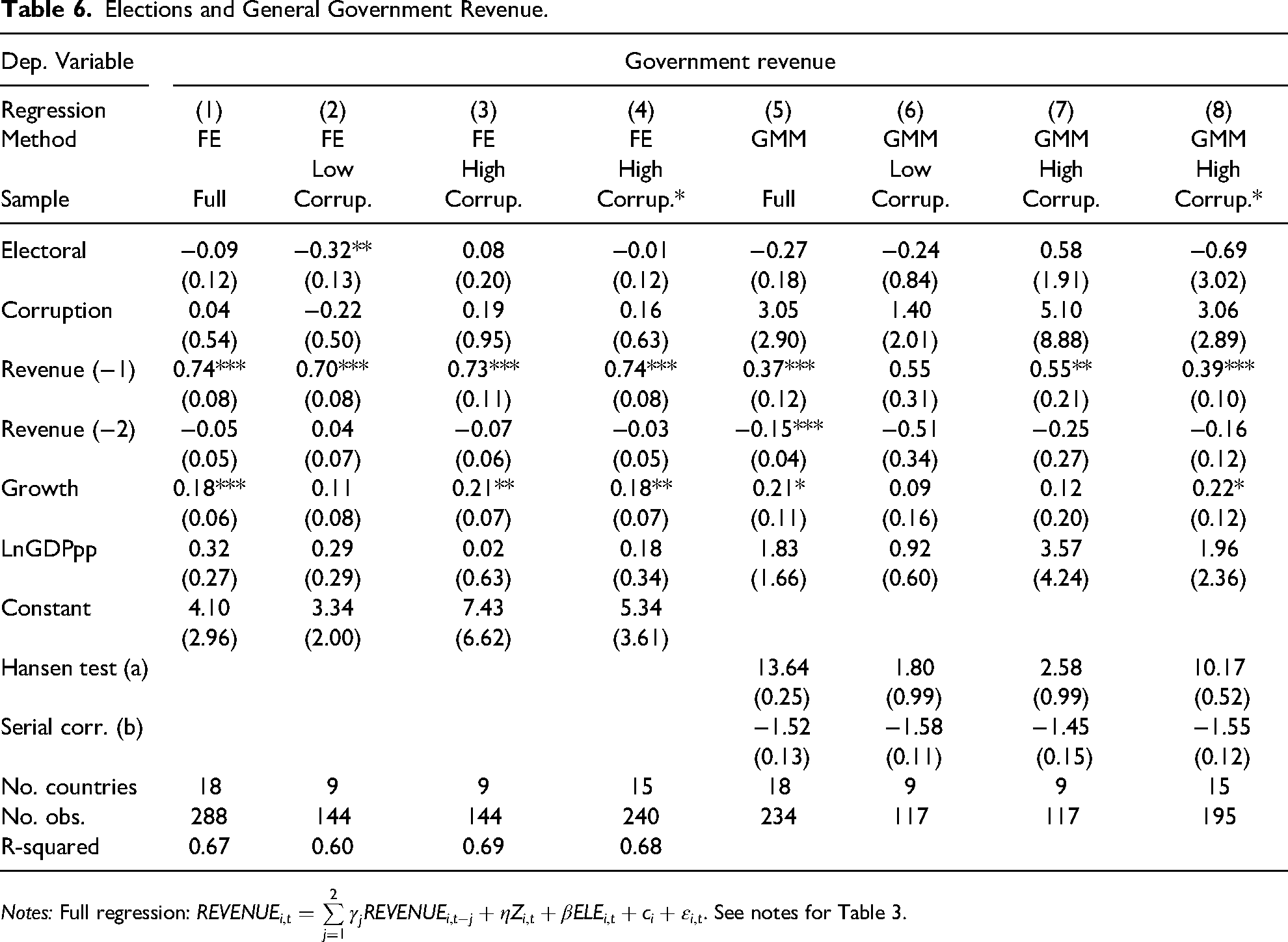
Notes: Full regression: $E X P E N D I T U R E_{i, t} = \sum_{j = 1}^{2} γ_{j} E X P E N D I T U R E_{i, t - j} + η Z_{i, t} + β E L E_{i, t} + c_{i} + ε_{i, t}$ . See notes for Table 3.

Finally, Table 6 presents the estimation results for government revenue. None of the results are significant except for the low corruption group, which suggests that Latin American politicians do not use the reduction of taxes during election year as a tool used to obtain votes.

Table 6.

Elections and General Government Revenue.

Dep. Variable	Government revenue
Regression	(1)	(2)	(3)	(4)	(5)	(6)	(7)	(8)
Method	FE	FE	FE	FE	GMM	GMM	GMM	GMM
Sample	Full	Low Corrup.	High Corrup.	High Corrup.*	Full	Low Corrup.	High Corrup.	High Corrup.*
Electoral	−0.09	−0.32**	0.08	−0.01	−0.27	−0.24	0.58	−0.69
	(0.12)	(0.13)	(0.20)	(0.12)	(0.18)	(0.84)	(1.91)	(3.02)
Corruption	0.04	−0.22	0.19	0.16	3.05	1.40	5.10	3.06
	(0.54)	(0.50)	(0.95)	(0.63)	(2.90)	(2.01)	(8.88)	(2.89)
Revenue (−1)	0.74***	0.70***	0.73***	0.74***	0.37***	0.55	0.55**	0.39***
	(0.08)	(0.08)	(0.11)	(0.08)	(0.12)	(0.31)	(0.21)	(0.10)
Revenue (−2)	−0.05	0.04	−0.07	−0.03	−0.15***	−0.51	−0.25	−0.16
	(0.05)	(0.07)	(0.06)	(0.05)	(0.04)	(0.34)	(0.27)	(0.12)
Growth	0.18***	0.11	0.21**	0.18**	0.21*	0.09	0.12	0.22*
	(0.06)	(0.08)	(0.07)	(0.07)	(0.11)	(0.16)	(0.20)	(0.12)
LnGDPpp	0.32	0.29	0.02	0.18	1.83	0.92	3.57	1.96
	(0.27)	(0.29)	(0.63)	(0.34)	(1.66)	(0.60)	(4.24)	(2.36)
Constant	4.10	3.34	7.43	5.34
	(2.96)	(2.00)	(6.62)	(3.61)
Hansen test (a)					13.64	1.80	2.58	10.17
					(0.25)	(0.99)	(0.99)	(0.52)
Serial corr. (b)					−1.52	−1.58	−1.45	−1.55
					(0.13)	(0.11)	(0.15)	(0.12)
No. countries	18	9	9	15	18	9	9	15
No. obs.	288	144	144	240	234	117	117	195
R-squared	0.67	0.60	0.69	0.68

Notes: Full regression: $R E V E N U E_{i, t} = \sum_{j = 1}^{2} γ_{j} R E V E N U E_{i, t - j} + η Z_{i, t} + β E L E_{i, t} + c_{i} + ε_{i, t}$ . See notes for Table 3.

Given the average fiscal deficit in the sample (2.56% of GDP), the GMM estimate implies that, on average, global fiscal deficit increases by 22.7% in election years. Meanwhile, primary fiscal deficit (0.44% of GDP) increases by 1.86% in election years. The difference between these two measures lies in the inclusion of interest payments. When interest payments are considered, the deficit increase in election years is much larger. A possible explanation for this is that debt does not change in election years, nor do interest payments. However, the deficit increases, which may be due to an increase in government expenditure.

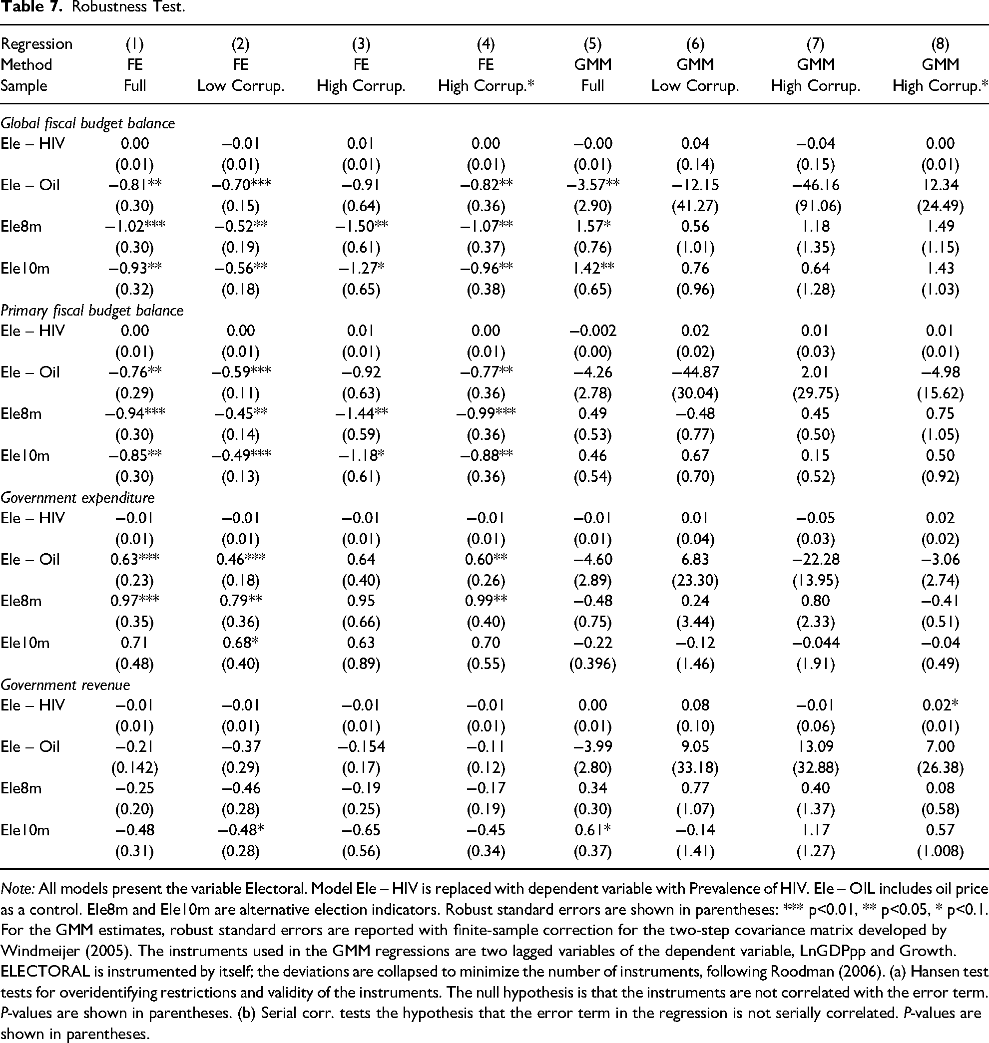
Robustness Checks

First, we change the dependent variable to a placebo variable to test whether the variable of interest affects one variable that it should not affect. Based on the data available for the 18 countries, the model is performed with the prevalence of HIV⁵ (% of the population ages 15–49) as the placebo variable.

Additionally, we include another covariate in the model to ensure that other variables are not useful and do not provide information about structural misspecifications (Lu and White 2014). The noncore variable chosen for comparison in the model was oil WTI price.⁶

Finally, following Shi and Svensson (2006), we run the model using alternative election indicators to capture possible differences in fiscal policies depending on the month of the election. For this purpose, we include two additional election dummies, ELE10m and ELE8m. ELE10m takes the value of one if an election takes place during the last 10 months in year t and the first 2 months of year $t + 1$ , and zero otherwise. ELE8 takes the value of one if an election takes place during the last 8 months in year t and the first 4 months of year $t + 1$ , and zero otherwise.

Table 7 presents the robustness test results. The results are consistent with the results regarding the four variables. Prevalence of HIV has no significant correlation with any variable, which confirms the absence of a spurious relationship in the model. Additionally, including oil price as a control does not change our initial findings. Finally, the alternative calculation of the election dummy does not differ from the results above. For example, for primary fiscal budget balance and GMM full sample, the results are significant for both ELE8m and ELE10m, with coefficient estimates of 0.49 and 0.46, respectively.

Table 7.

Robustness Test.

Regression	(1)	(2)	(3)	(4)	(5)	(6)	(7)	(8)
Method	FE	FE	FE	FE	GMM	GMM	GMM	GMM
Sample	Full	Low Corrup.	High Corrup.	High Corrup.*	Full	Low Corrup.	High Corrup.	High Corrup.*
Global fiscal budget balance
Ele – HIV	0.00	−0.01	0.01	0.00	−0.00	0.04	−0.04	0.00
	(0.01)	(0.01)	(0.01)	(0.01)	(0.01)	(0.14)	(0.15)	(0.01)
Ele – Oil	−0.81**	−0.70***	−0.91	−0.82**	−3.57**	−12.15	−46.16	12.34
	(0.30)	(0.15)	(0.64)	(0.36)	(2.90)	(41.27)	(91.06)	(24.49)
Ele8m	−1.02***	−0.52**	−1.50**	−1.07**	1.57*	0.56	1.18	1.49
	(0.30)	(0.19)	(0.61)	(0.37)	(0.76)	(1.01)	(1.35)	(1.15)
Ele10m	−0.93**	−0.56**	−1.27*	−0.96**	1.42**	0.76	0.64	1.43
	(0.32)	(0.18)	(0.65)	(0.38)	(0.65)	(0.96)	(1.28)	(1.03)
Primary fiscal budget balance
Ele – HIV	0.00	0.00	0.01	0.00	−0.002	0.02	0.01	0.01
	(0.01)	(0.01)	(0.01)	(0.01)	(0.00)	(0.02)	(0.03)	(0.01)
Ele – Oil	−0.76**	−0.59***	−0.92	−0.77**	−4.26	−44.87	2.01	−4.98
	(0.29)	(0.11)	(0.63)	(0.36)	(2.78)	(30.04)	(29.75)	(15.62)
Ele8m	−0.94***	−0.45**	−1.44**	−0.99***	0.49	−0.48	0.45	0.75
	(0.30)	(0.14)	(0.59)	(0.36)	(0.53)	(0.77)	(0.50)	(1.05)
Ele10m	−0.85**	−0.49***	−1.18*	−0.88**	0.46	0.67	0.15	0.50
	(0.30)	(0.13)	(0.61)	(0.36)	(0.54)	(0.70)	(0.52)	(0.92)
Government expenditure
Ele – HIV	−0.01	−0.01	−0.01	−0.01	−0.01	0.01	−0.05	0.02
	(0.01)	(0.01)	(0.01)	(0.01)	(0.01)	(0.04)	(0.03)	(0.02)
Ele – Oil	0.63***	0.46***	0.64	0.60**	−4.60	6.83	−22.28	−3.06
	(0.23)	(0.18)	(0.40)	(0.26)	(2.89)	(23.30)	(13.95)	(2.74)
Ele8m	0.97***	0.79**	0.95	0.99**	−0.48	0.24	0.80	−0.41
	(0.35)	(0.36)	(0.66)	(0.40)	(0.75)	(3.44)	(2.33)	(0.51)
Ele10m	0.71	0.68*	0.63	0.70	−0.22	−0.12	−0.044	−0.04
	(0.48)	(0.40)	(0.89)	(0.55)	(0.396)	(1.46)	(1.91)	(0.49)
Government revenue
Ele – HIV	−0.01	−0.01	−0.01	−0.01	0.00	0.08	−0.01	0.02*
	(0.01)	(0.01)	(0.01)	(0.01)	(0.01)	(0.10)	(0.06)	(0.01)
Ele – Oil	−0.21	−0.37	−0.154	−0.11	−3.99	9.05	13.09	7.00
	(0.142)	(0.29)	(0.17)	(0.12)	(2.80)	(33.18)	(32.88)	(26.38)
Ele8m	−0.25	−0.46	−0.19	−0.17	0.34	0.77	0.40	0.08
	(0.20)	(0.28)	(0.25)	(0.19)	(0.30)	(1.07)	(1.37)	(0.58)
Ele10m	−0.48	−0.48*	−0.65	−0.45	0.61*	−0.14	1.17	0.57
	(0.31)	(0.28)	(0.56)	(0.34)	(0.37)	(1.41)	(1.27)	(1.008)

Note: All models present the variable Electoral. Model Ele – HIV is replaced with dependent variable with Prevalence of HIV. Ele – OIL includes oil price as a control. Ele8m and Ele10m are alternative election indicators. Robust standard errors are shown in parentheses: *** p<0.01, ** p<0.05, * p<0.1. For the GMM estimates, robust standard errors are reported with finite-sample correction for the two-step covariance matrix developed by Windmeijer (2005). The instruments used in the GMM regressions are two lagged variables of the dependent variable, LnGDPpp and Growth. ELECTORAL is instrumented by itself; the deviations are collapsed to minimize the number of instruments, following Roodman (2006). (a) Hansen test tests for overidentifying restrictions and validity of the instruments. The null hypothesis is that the instruments are not correlated with the error term. P-values are shown in parentheses. (b) Serial corr. tests the hypothesis that the error term in the regression is not serially correlated. P-values are shown in parentheses.

Discussion

Our results show that elections have a positive effect on expenditure and a negative effect on revenue and fiscal balance, consistent with the theoretical predictions. However, similar to the results of Mandon and Cazals (2019), we do not find strong statistical evidence of pre-electoral manipulation of revenue and expenditure (significant only for FE), but we do find statistically significant and robust manipulation of fiscal balance.

Mandon and Cazals (2019) explain that these results are due to two reasons: (i) the fiscal balance systematically deteriorates before elections, and (ii) the mechanisms are not clear because the strategy of incumbents is context-dependent. Specifically, depending on political context, easiness and pay-off that leaders face, they may favor manipulation of either revenue or spending. Thus, incumbents may adopt a revenue strategy, expenditure strategy, or mixed strategy.

Furthermore, our results reveal systematic differences between countries with high and low corruption indexes. Countries with higher corruption levels show a stronger negative relationship between elections and fiscal balance. Higher corruption leads to higher rents, and higher rents cause PBCs according to Shi and Svensson (2006).

Our model concludes that the higher politicians’ rents of remaining in power, the more incentivized they are to increase spending or manipulate fiscal tools so that they can improve their chances of getting re-elected. By contrast, a greater share of informed voters creates the opposite effect. More informed voters cause a smaller cycle because fewer voters can be influenced or manipulated by a pre-electoral boom.

This study focuses only on the corruption index; however, other studies identify different institutional factors that affect the existence of PBCs. Gonzalez (2002) explains the strong emergence of PBCs in “imperfect democracies” compared with well-developed political systems. They reveal a link between election cycles and a country's “index of democracy,” which is the cost for voters when making a decision to vote, and the “index of transparency,” which measures the magnitude of the economy's information asymmetry. Therefore, the lack of democracy may generate greater incentives for cycles to emerge.

Strong fiscal frameworks can increase tax collection, limit public expenditure, and guarantee sustainable fiscal policies (Balibek et al. 2019). However, these rules will be effective only when a government functions well and maintains a clearly defined budgetary framework (Celik, Kose and Ohnsorge 2020). Several studies examine different factors that may contribute to PBCs or the lack of PBCs. For example, Gootjes, de Haan and Jong-A-Pin (2021) investigate whether fiscal rules constrain PBCs and conclude that strong fiscal rules lessen PBCs. The results indicate that fiscal rules have a stronger effect in countries with veto player, left-wing governments, established democracies, and more globalized economies. Future research could explore the effect of fiscal rules and the incumbent's ideological orientation on the probability of PBCs.

Veiga, Veiga and Morozumi (2017) study the circumstances under which fiscal manipulation may occur. They find that the main condition that favors the existence of PBCs is the degree of media freedom; budget deficits are stronger when media freedom is weaker. Fiscal rules are important mechanisms for preventing or reducing PBCs. Furthermore, fiscal rules are an institutional factor and, as the literature and our results establish, institutional factors determine the existence of PBCs.

Accordingly, an important question is whether Uruguay, Chile, and Costa Rica have institutional factors that may differentiate them from other Latin American countries. Delgado (2018) analyze the three countries’ democracies and find that they have the highest quality of democracy in Latin America based on different reports and indexes. They state that the principal variable explaining the quality of democracy is the political party system.

Conclusions

This study has two contributions to the literature on PBCs. First, we provide an up-to-date empirical analysis of PBCs in Latin America, differentiated by global and primary fiscal balances. We find that the government's global fiscal deficit increases by 0.6 percentage points as a share of GDP in election years, while primary fiscal deficit increases by 0.8 percentage points as a share of the GDP in election years.

Second, we show that PBCs are much larger in countries with a high corruption index than in those with a low corruption index. For countries with a low corruption index, the global fiscal deficit increases by 0.5 percentage points and primary fiscal deficit increases by 0.4 percentage points, both as a share of GDP in election years. Meanwhile, for countries with a high corruption index, the global fiscal deficit increases by 1.24 percentage points and the primary fiscal deficit increases by 1.26 percentage points, both as a share of GDP and in election years. The results significantly differ in that PBCs in high-corruption countries are more than double that in low-corruption countries.

This study shows the existence of PBCs, with great differences between countries in Latin America. These differences can be explained by corruption. The results support the findings of previous literature, which states PBCs depend on the country's institutional factors, and politicians manipulate fiscal tools before elections. Therefore, political factors and fiscal decisions must be considered when analyzing business cycles.

Footnotes

Declaration of Conflicting Interests

The authors declared no potential conflicts of interest with respect to the research, authorship, and/or publication of this article.

Funding

The authors received no financial support for the research, authorship, and/or publication of this article.

ORCID iDs

Maí Suárez

Nicolás Acosta-González

Notes

Author Biographies

Maí Suárez is an economist whose research focuses on development and inequality.

Nicolás Acosta-González is a professor of Econometrics at Pontificia Universidad Católica del Ecuador. His area of interest is applied econometrics and impact evaluation.

References

Acemoglu

Daron

Johnson

Simon

Robinson

James A

. 2015. Las instituciones como causa fundamental del crecimiento a largo plazo. In: CAF (Ed.), Economía Política del Crecimiento, Cadenas causales y mecanismos institucionales. Gestión Pública y Desarrollo de América Latina, Buenos Aires, pp. 191–321.

Aktas

E. E.

2021. “Dynamic Effects of Corruption on General Government Final Consumption Expenditure: Evidence from OECD Countries.” Public Finance Quarterly= Pénzügyi Szemle 66 (4): 551–567. https://doi.org/10.35551/PFQ_2021_4_6.

Alesina

Alberto

Campante

Filipe R.

Tabellini

Guido

. 2008. “Why is Fiscal Policy Often Procyclical?” Journal of the European Economic Association 6 (5): 1006–1036. https://doi.org/10.1162/JEEA.2008.6.5.1006.

Alesina

Paradisi

. 2017. “Political Budget Cycles: Evidence from Italian Cities.” Economics & Politics 29 (2): 157–177. https://doi.org/10.1111/ecpo.12091.

Ames

Barry

. 1987. “The Congressional Connection: The Structure of Politics and the Distribution of Public Expenditures in Brazil's Competitive Period.” Comparative Politics 19 (2): 147–171. https://doi.org/10.2307/421796.

Arellano

Manuel

Bond

Stephen

. 1991. “Some Tests of Specification for Panel Data: Monte Carlo Evidence and an Application to Employment Equations.” Review of Economic Studies 58: 277–297. https://doi.org/10.2307/2297968.

Arellano

Manuel

Bover

Olympia

. 1995. “Another Look at the Instrumental Variable Estimation of Error-Components Models.” Journal of Econometrics 68 (1): 29–51. https://doi.org/10.1016/0304-4076(94)01642-D.

Balibek

M. E.

Haque

M. T.

Rivetti

Tamene

M. M.

. 2019. Medium-Term Debt Management Strategy: Analytical Tool Manual. International Monetary Fund.

Barberia

Lorea

Avelino

George

. 2011. “Do Political Budget Cycles Differ in Latin American Democracies?” Economía 11 (2): 101–134. 10.1353/eco.2011.0001.

10.

Blundell

Richard

Bond

Stephen

. 1998. “Initial Conditions and Moment Restrictions in Dynamic Panel Data Models.” Journal of Econometrics 87: 115–143. https://doi.org/10.1016/S0304-4076(98)00009-8.

11.

Brender

Adi

Drazen

Allan

. 2005. “Political Budget Cycles in New Versus Established Democracies.” Journal of Monetary Economics 52 (7): 1271–1295. https://doi.org/10.1016/j.jmoneco.2005.04.004.

12.

Celik

Kose

M. A.

Ohnsorge

. 2020. Subdued potential growth: Sources and remedies. CAMA Working Paper No.24/2020.

13.

Chong

S. P. C.

Tee

C. M.

Cheng

S. V.

. 2020. “Political Institutions and the Control of Corruption: A Cross-Country Evidence.” Journal of Financial Crime 28 (1): 26–48. https://doi.org/10.1108/JFC-05-2020-0094.

14.

Cooray

Özmen

. 2024. “The Role of Institutions on Public Debt: A Quantile Regression Approach.” International Review of Economics & Finance 93: 912–928. https://doi.org/10.1016/j.iref.2024.03.065.

15.

Delgado

Rafael G. M

. 2018. “Democracia de alta Calidad en América Latina. Análisis Histórico Comparado Entre Chile, Costa Rica y Uruguay.” Política. Revista de Ciencia Política 56 (1): 89–106. https://doi.org/10.5354/0719-5338.2018.58135

16.

Destek

M. A.

Adedoyin

Bekun

F. V.

Aydin

. 2023. “Converting a Resource Curse into a Resource Blessing: The Function of Institutional Quality with Different Dimensions.” Resources Policy 80: 103234. https://doi.org/10.1016/j.resourpol.2022.103234.

17.

Drazen

Allan

Marcela

Eslava

. 2010. “Electoral Manipulation via Voter-Friendly Spending: Theory and Evidence.” Journal of Development Economics 92 (1): 39–52.

18.

Eslava

. 2006. “Ciclos políticos de la política fiscal con votantes opuestos al déficit.” El caso colombiano. El trimestre económico 73 (290): 289–336.

19.

Gonzalez

Maria D. L. A

. 2002. On democracy, transparency and economic policy: Theory and evidence. Princeton University.

20.

Gootjes

Bram

de Haan

Jakob

Jong-A-Pin

Richard

. 2021. “Do Fiscal Rules Constrain Political Budget Cycles?” Public Choice 188: 1–30. https://doi.org/10.1007/s11127-020-00797-3.

21.

Janků

Libich

. 2019. “Ignorance Isn't Bliss: Uninformed Voters Drive Budget Cycles.” Journal of Public Economics 173: 21–43.

22.

Kwakwa

P. A.

Aboagye

. 2024. “Addressing Africa’s Carbon Dioxide Emission: The Role of Natural Resources, Control of Corruption, Voice and Accountability and Regulatory Quality.” Management of Environmental Quality: An International Journal 35 (7): 1437–1460. https://doi.org/10.1108/MEQ-11-2023-0381.

23.

López

Sandoval

Ignacio

. 2016. “Elección Pública y Análisis Institucional de la Acción Gubernamental.” Economía Informa 396: 49–66. https://doi.org/10.1016/j.ecin.2016.01.003

24.

Xun

White

Halbert

. 2014. “Robustness Checks and Robustness Tests in Applied Economics.” Journal of Econometrics 178 (1): 194–206. https://doi.org/10.1016/j.jeconom.2013.08.016.

25.

Mandon

Pierre

Cazals

Antoine

. 2019. “Political Budget Cycles: Manipulation by Leaders Versus Manipulation by Researchers? Evidence from a Meta-Regression Analysis.” Journal of Economic Surveys 33 (1): 274–308. https://doi.org/10.1111/joes.12263.

26.

Mejía-Acosta

Coppedge

. 2001. “Political determinants of fiscal discipline in Latin America, 1979-1998.” International Congress of the Latin American Studies Association, Marriott Wardman Park Hotel, Washington, DC.

27.

Moschovis

2010. “Public Spending Allocation, Fiscal Performance and Corruption.” Economic Papers: A Journal of Applied Economics and Policy 29 (1): 64–79. https://doi.org/10.1111/j.1759-3441.2010.00048.x.

28.

Musgrave

Richard A

. 1973. Public Finance in Theory and Practice. Kogakusa: McGraw-Hill. The Mechanism of Political Budget Cycles in Greece.

29.

Nguyen

T. C.

Tran

T. L.

. 2023. “The Political Budget Cycles in Emerging and Developing Countries.” Journal of Economics and Development 25 (3): 205–225. https://doi.org/10.1108/JED-01-2023-0015.

30.

Petrakos

Rontos

Salvati

Vavoura

Vavouras

. 2021. “Toward a Political Budget Cycle? Unveiling Long-Term Latent Paths in Greece.” Quality & Quantity 56: 3379–3394. https://doi.org/10.1007/s11135-021-01260-1.

31.

Roodman

David

. 2006. “How to do xtabond2: An introduction to Difference and System GMM in Stata.” The Stata Journal 9 (1): 86–136. https://doi.org/10.1177/1536867X0900900106

32.

Schuknecht

Ludger

. 2000. “Fiscal Policy Cycles and Public Expenditure in Developing Countries.” Public Choice 102: 113–128. https://doi.org/10.1023/A:1005026806998.

33.

Shi

Min

Svensson

Jakob

. 2006. “Political Budget Cycles: Do They Differ Across Countries and why?” Journal of Public Economics 90 (8-9): 1367–1389. https://doi.org/10.1016/j.jpubeco.2005.09.009v.

34.

Sironi

Tornari

. 2013. “Corruption, Political Instability and Public Finance in Europe.” International Journal of Monetary Economics and Finance 6 (2–3): 203–212. https://doi.org/10.1504/IJMEF.2013.056397.

35.

Stolfi

Hallerberg

. 2016. “Clientelistic Budget Cycles: Evidence from Health Policy in the Italian Regions.” Journal of European Public Policy 23 (6): 833–850. https://doi.org/10.1080/13501763.2015.1075577.

36.

Streb

Jorge M.

Lema

Daniel

Torrens

Gustavo

. 2009. “Checks and Balances on Political Budget Cycles: Cross-Country Evidence.” Kyklos 62 (3): 426–447.

37.

Udemba

N. E.

Onyenegecha

Olasehinde-Williams

. 2022. “Institutional Transformation as an Effective Tool for Reducing Corruption and Enhancing Economic Growth: A Panel Study of West African Countries.” Journal of Public Affairs 22 (2): e2389.

38.

Veiga

Francisco J.

Veiga

Linda G.

Morozumi

Atsuyoshi

. 2017. “Political Budget Cycles and media Freedom.” Electoral Studies 45: 88–99. https://doi.org/10.1016/j.electstud.2016.11.008.

39.

Windmeijer

Frank

. 2005. “A Finite Sample Correction for the Variance of Linear Efficient two-Step GMM Estimators.” Journal of Econometrics 126 (1): 25–51. https://doi.org/10.1016/j.jeconom.2004.02.005.

40.

Wolfers

Justin

. 2002. Are voters rational?: Evidence from gubernatorial elections. Working Paper No. 1730. Stanford: Graduate School of Business, Stanford.

41.

World Bank. 2024. World Governance indicators. https://www.worldbank.org/en/publication/worldwide-governance-indicators.