
Abstract
It is well known that corruption is harmful to the economy. Corruption's effect on the sectoral composition of economic activity, however, is comparatively understudied. We examine the relationship between corruption and the distribution of employment and establishments across sectors in Brazilian municipalities. We test whether the shares of employees and establishments across sectors are influenced by the amount of corruption in the area. We also test whether sectors are more concentrated in general using an employment share weighted HHI measure. We find that there are larger shares of employment and establishments in the relatively non-corrupt agricultural sector in highly corrupt areas and, likewise, lower shares of employment/establishments in relative corruption-prone sectors (e.g., construction). Our strongest evidence of the impact of corruption is shown through market concentration, where concentration is higher in more corrupt municipalities across every sector.
Introduction
There are many proposed mechanisms through which corruption is hypothesized to reduce growth and harm the productive capacity of an economy. These mechanisms range from uncertainty (Wei 1997; Campos, Lien and Pradhan 1999; Bologna Pavlik 2018) 1 to a weakened property rights system (Klitgaard 2000; Hogdson and Jiang 2007) and a misallocation of resources, broadly construed. 2 Our focus is on this last mechanism—specifically, how corruption is associated with the sectoral composition of firms and employment resulting from decentralized entry and participation decisions.
Sectoral composition could be affected directly via individual choice (labor choice) or indirectly through broader market conditions. On the one hand, the potential for illegal rents may attract entrepreneurs to sectors that are prone to corruption. 3 Here we may expect more business activity to take place in sectors that are particularly susceptible to corruption. Boudreaux, Nikolaev and Holcombe (2018) find evidence of this in the U.S. However, corruption may also limit entry and monopolize these sectors—as monopolized rents yield the highest return (Bliss and Di Tella 1997; Ades and Di Tella 1999; Emerson 2006). Moreover, if corruption does not grease the wheels of economic growth, we may see firms and/or individuals avoiding these particularly corrupt sectors altogether. In the language of Baumol (1990), corruption could be attracting unproductive (or potentially destructive) entrepreneurs while simultaneously deterring productive entrepreneurship, making the net effect of corruption on sector-specific business activity an empirical question.
In this paper, we study how corruption affects the composition of business activity in the context of Brazil. We first examine whether corruption is associated with differences in the sectoral distribution of labor, by analyzing how corruption correlates with the share of total employment across nine sectors. Four of these sectors (wholesale, manufacturing, construction, and transportation and communication) are known to be prone to corruption internationally. The first—wholesale—is identified by Colonnelli and Prem (2022) as one of the top sectors experiencing corruption in Brazil. The latter three are cited in the Organization for Economic Development and Cooperation (OECD) Foreign Bribery Report (2014) as being particularly corrupt globally. The next four sectors (education, health, professional services, and agriculture) are generally considered to be non-corrupt (Boudreaux, Nikolaev and Holcombe 2018; Colonnelli and Prem 2022), though there is reason to believe there is room for corruption in the first three in Brazil. 4 The final sector is public administration. Whereas the first eight sectors are focused on tangible good/service producing activities and can include government providers 5 , the latter sector is focused on the less tangible administrative services of government alone (e.g., defense, social security, etc.). If corruption is associated with a higher employment share in this sector, it could suggest bureaucratic bloat. We calculate employment shares using the Relação Anual de Informações Sociais (RAIS)—a dataset containing the universe of formal firms in Brazil. 6
As a second step in our analysis, we study how corruption affects establishment shares across the same nine sectors. Although closely related to employment shares, establishment shares provide additional information about the types of firms operating locally and are more directly indicative of entrepreneurial activity. A key result in Colonnelli and Prem (2022) is that, following an exogenous reduction in corruption, the number of firms increase in government-dependent sectors, while other sectors remain largely unaffected. In our context, this finding would imply that more corrupt areas exhibit a smaller share of establishments in corruption-prone sectors. Such a pattern would be consistent with distorted entry and sorting across sectors induced by corruption, rather than government directed allocation, whereby entrepreneurial activity is disproportionately concentrated in sectors that are less exposed to corrupt interactions.
Lastly, we construct a Herfindahl–Hirschman Index (HHI) using establishments’ employment shares—as opposed to market shares—for each sector-municipality pair. This measure allows us to study how corruption is related not only to the distribution of activity across sectors, but also to the degree of concentration (competition) within sectors. This distinction is important because even if certain sectors exhibit lower employment or fewer establishments overall, economic activity within those sectors may nevertheless be highly concentrated among a small number of firms. Higher concentration may reflect barriers to entry or competitive distortions associated with corruption, rather than shifts in activity across industries per se. In this case, corruption would be associated with reduced competitive pressure and fewer opportunities for small-scale or entrant firms, even holding the sectoral composition of activity fixed. Both mechanisms may operate simultaneously. For example, if corruption-prone sectors are both relatively small and more concentrated, while less corruption-prone sectors remain more competitive, this would be consistent with corruption shaping economic activity through both sectoral sorting and within-sector concentration.
Our primary corruption measure comes from Avis, Ferraz and Finan (2018). In their paper, they measure corruption across all Brazilian municipalities that were selected for a corruption audit between 2006 and 2013. This audit program relied on the random selection of municipalities, focused on auditing the (mis)use of federal transfers, and publicized the results of each audit so that the public would be made aware of any malfeasance. 7 They utilize the 2006–2013 audit reports to calculate the number of instances corruption was uncovered; the audits themselves cover multiple years of transfers and thus this is best interpreted as a cross-sectional measure for our analysis. Because municipalities vary drastically in size, we take this number and divide it by the municipality's population for a measure of “corruption per capita”. This measure is available for 935 (of 5,565) municipalities.
Our main results show that employment shares across seven of the eight good/service producing sectors are lower in municipalities with higher levels of corruption. Of these eight, the only sector that sees higher employment shares is agriculture. We also see that public administration shares are larger. Likewise, for establishment shares, most sectors experience a reduction in their share except for agriculture and public administration. These results hold both with and without controls aiming to capture the general level of development in the municipality (GDP per capita, size of informality, density, etc.); all estimates also include state and audit fixed effects.
That agricultural shares increase in response to more corruption is consistent with a “sand the wheels” effect of corruption in Brazil. Using the same audit program, Colonnelli and Prem (2022) identify the 50 most and least corrupt sectors. Agricultural activities frequently appear in their 50 least corrupt list (e.g., grape growing, raising of large animals, and saltwater fishing). In contrast, activities in the other seven good/servicing producing sectors appear at least once in the most corrupt list, including wholesale of pharmaceutical products, construction of road and railroad, manufacture of medicines, road passenger transport, hospital care activities, school transportation, and credit card management. Consistent with this, we observe relatively more firms and workers operating in agriculture and relatively fewer in sectors that are more exposed to corruption. We also observe a higher share of employment and establishments in public administration in more corrupt municipalities, consistent with an expansion of administrative activity rather than productive goods and services. Taken together, these patterns suggest that corruption reshapes the sectoral composition of economic activity, shifting firms and workers toward less corruption-exposed activities and toward administrative functions of government.
Our strongest evidence, however, points to economy-wide distortions in market structure. We find that higher corruption is associated with increased concentration across all nine sectors, as measured by our employment-share HHI. This effect is strongest in professional services (a 40% increase in HHI), wholesale (39%), and manufacturing (36%)—all sectors that are plausibly exposed to corruption in Brazil. However, concentration also increases by 33% in agriculture, a sector typically viewed as relatively less corruption-prone. These results suggest that corruption is associated with higher concentration even in sectors where activity appears to shift away from direct corrupt interactions, implying that no sector is fully insulated from its effects. The economy-wide increase in concentration is consistent with reduced entry and diminished small-scale entrepreneurial activity, particularly among firms that are most likely to engage in productive entrepreneurship (Baumol 1990).
In addition to the standard robustness checks (e.g., alternative datasets, controls, and time periods) these latter results are robust to an instrumental variable analysis where we instrument for corruption per capita using measures of political participation (number of local councils and the number of appointed local councils) 8 and a measure of management capacity. 9 These measures all date back to 1998, several years prior to the audit program. The first two instruments aim to capture the degree to which the local population is engaged in government affairs, with the idea that increased engagement of the voting population can reduce corruption. The last instrument is essentially a management capacity indicator. It captures the extent to which a municipality has districts, subdivisions, zoning plans/laws, and other building codes/codes of conduct. The laws and plans included in this management indicator are relatively complex and signify that the local government is relatively well-functioning, likely with less corruption. Thus, all three instruments are likely strong, negative, predictors of corruption per capita, and we indeed find that this is the case.
We also believe that these three indicators are plausibly exogenous to the extent that they only impact concentration through their effect on corruption. First, in terms of reverse causality, these instruments were in place well before the audits occurred. We are using data from 1998 and thus if the corruption uncovered did encourage the creation of new councils and/or management rules, we are not capturing that here. Second, it is difficult to see how the existence and activity of local councils—on its own—could impact sectoral concentration. These councils exist for the purpose of citizen engagement in government affairs. The management indicator is perhaps suspect as certain sectors may be more sensitive to zoning laws/codes. However, we note that controlling for acts of mis-management—constructed from the same Avis, Ferraz and Finan (2018) dataset—seems to have little to no effect on our corruption coefficient for HHI measures. 10 This mismanagement measure captures instances of misconduct, such as not filling out a document properly, without any evidence of corruption. Thus, corruption is an important predictor even after controlling for a more rule-based measure of misconduct. Nevertheless, as with all instrumental variables analyses, these results should be interpreted with caution. We instrument for corruption using each indicator separately and then together, finding our most robust estimates to be remarkably stable across the four specifications. 11
The remainder of this paper is as follows. A review of the literature is given in Section Corruption, Entrepreneurship, and Sectoral Competition, along with theoretical discussions concerning the corruption-sectoral composition relationship. An overview of the audit program and corruption in Brazil is given in Section Brazil’s Random Audit Program & Most Corruption-Prone Sectors. Data are discussed in Section Data. Section Results summarizes the empirical method and results. Section Conclusion concludes.
Corruption, Entrepreneurship, and Sectoral Competition
Corruption and Entrepreneurship
A large literature examines the relationship between corruption, firms, and entrepreneurship (Desai, Gompers and Lerner 2003; Ovaska and Sobel 2005; Avnimelech, Zelekha and Sharabi 2014; Boudreaux 2014; Chowdhury, Terjesen and Audretsch 2015; Bologna and Ross 2015; Colonnelli and Prem 2022). Despite wide variation in scope, setting, and empirical approach, this literature consistently finds that corruption reduces entrepreneurship and/or business activity. A related debate considers whether corruption may, in certain institutional environments, partially offset excessive formal barriers to operation—the so-called “grease the wheels” hypothesis (e.g., Dreher and Gassebner 2013). Nevertheless, Dutta and Sobel (2016) show that even in environments with poor business climates, where corruption may be relatively less harmful, the net effect of corruption on entrepreneurial activity remains negative.
While this literature has largely focused on aggregate outcomes—such as the total number of firms or entrepreneurs—much less is known about how corruption shapes the sectoral composition and market structure of economic activity. Understanding these dimensions is important, as corruption may affect not only how much entrepreneurial activity occurs, but also where it occurs and how it is organized across and within sectors.
Our paper most closely relates to Boudreaux, Nikolaev and Holcombe (2018) in their analysis of establishment shares; and to Bologna and Ross (2015) and Colonnelli and Prem (2022) in their focus on Brazil. Boudreaux, Nikolaev and Holcombe (2018) examine the relationship between corruption convictions per capita and establishment shares across U.S. states, finding that states with higher conviction rates have a larger share of firms in construction and smaller shares in non-profit and education sectors. They interpret these results as evidence that corruption attracts business activity toward more corruption-prone sectors.
As alluded to in the introductory section, the findings of Boudreaux, Nikolaev and Holcombe (2018) differ from ours. Rather than viewing this contrast as a contradiction, we interpret it as highlighting important differences in measurement and institutional context across settings. In particular, we offer two potential explanations for this difference. First, the corruption measure used in Boudreaux, Nikolaev and Holcombe (2018) relies on the capacity of the U.S. legal system to detect and prosecute corruption, which may be correlated with the scale of construction activity itself. Our measure, discussed in detail in Section The Random Audit Program, is broader in scope and less directly tied to enforcement ability, making it less susceptible to this form of endogeneity. Second, as argued in Dreher and Schneider (2010), corruption in high-income countries such as the United States is likely to be less coercive. In such settings, bribery perceived as unfair may be challenged through legal channels, reducing its deterrent effect on productive firms. In Brazil, by contrast, corrupt interactions are more likely to be coercive and less easily contested via the legal system, making participation in corruption-prone sectors relatively less attractive to productive entrepreneurs.
In the Brazilian context, Bologna and Ross (2015) use a similar cross-sectional corruption measure derived from the random audit program to estimate corruption's effect on the number of establishments across municipalities, finding that corruption is harmful to business activity. Colonnelli and Prem (2022) take a different approach by studying the audits themselves and show that audit-induced reductions in corruption increase the number of establishments in government-dependent sectors, with little effect elsewhere. Taken together, these studies provide strong evidence that corruption reduces the overall number of establishments in Brazilian municipalities. Our contribution differs in that we examine how corruption is associated with the distribution of economic activity across sectors and the market structure within sectors.
Corruption, Sectoral Composition, and Competition
As emphasized by Baumol (1990), although the total number of entrepreneurs may vary across societies, the distribution of entrepreneurial effort across productive, unproductive, and destructive activities may be even more consequential for economic growth. Using similar logic, entrepreneurs can sort across sectors given differing associated institutional factors, like corruption. Our focus is on this latter effect.
Corruption can influence sectoral composition through several, potentially offsetting, mechanisms. On the one hand, sectors that involve frequent interaction with government, discretionary regulation, and/or large public contracts may offer greater opportunities for rent extraction. We refer to such industries as “corruption-prone”. 12 In these settings, corruption could attract entrepreneurs toward these sectors, increasing establishment and employment shares in corruption-prone activities. On the other hand, corruption may raise effective entry costs, increase uncertainty, and expose firms and workers to coercive demands by officials. When corruption is sufficiently costly or unpredictable, productive entrepreneurs may instead avoid these sectors, shifting activity toward industries that are less exposed to corrupt interactions. From an individual choice perspective, then, the net effect of corruption on sectoral composition is an empirical question.
The foregoing discussion frames corruption primarily as influencing “sectoral choice” by workers, firms, and/or entrepreneurs. Corruption may also, however, affect the market structure of sectors, with implications for sectoral outcomes as well. Corrupt officials can limit entry, protect incumbents, and facilitate collusive arrangements, leading to higher concentration even when overall economic activity declines. 13 An increase in concentration may therefore reflect reduced competition and fewer opportunities for small-scale or entrant firms, particularly those engaged in productive entrepreneurship. Importantly, a decline in the number of firms does not, by itself, reveal how economic activity is distributed among remaining establishments, making within-sector concentration a distinct and complementary margin of adjustment.
Guided by these mechanisms, our empirical analysis examines two related dimensions: (i) how corruption is associated with the sectoral composition of employment and establishments, and (ii) how corruption relates to within-sector concentration across municipalities. Together, these outcomes provide a richer picture of how corruption relates to economic activity beyond its effects on aggregate firm counts.
Historical Determinants of Sectoral Composition
A natural concern with the above discussion (and, more specifically, with our cross-sectional analysis) is that sectoral composition may be predetermined by historical, geographic, or technological factors; these factors might also influence contemporary corruption. For example, municipalities that are predominantly agrarian likely have a larger share of their economy dedicated to agriculture, regardless of municipal corruption. Agrarian municipalities might also have less rents available for extraction and therefore less corruption. This raises two related concerns. First, changes in contemporary corruption could have little scope to influence sectoral composition if it is largely predetermined. Second, any observed correlation between corruption and sectoral composition may be driven, at least in part, by historical or geographical factors rather than a meaningful causal relationship between contemporary corruption and economic activity. While the first concern is directly testable and is the central focus of our empirical analysis, addressing the second requires additional theoretical clarification. We therefore use this section to expand on these ideas and to motivate why corruption may be systematically related to sectoral composition and market structure, even in a cross-sectional setting.
Returning to the agrarian example, some municipalities are geographically predisposed to having a relatively large of agricultural sector. If agricultural markets are assumed to be highly competitive and that competition is assumed to reduce corruption, this could generate a negative long-run association between corruption and agricultural employment or establishments shares. Importantly, such an association would not imply a causal effect of corruption on sectoral composition. However, both assumptions underlying this argument—that agricultural markets are competitive and that competition (lower rents) uniformly reduces corruption—are subject to important caveats.
First, the degree of competition in agriculture depends critically on context and on whether competition is evaluated at the sectoral level or at the level of individual farmers. Although agriculture is often used to motivate models of perfect competition in introductory economics, the effective degree of competition in agricultural markets has long been debated (Johnson 1954; Sykuta 2013). More recently, Moon (2022) argues that there is a lack of dynamic competition in agriculture. Thus, it is not clear that agricultural markets are always competitive.
Second, the relationship between competition and corruption is complex, conditional, and bidirectional. A substantial literature links market competition, rents, and corruption (e.g., Bliss and Di Tella 1997; Ades and Di Tella 1999; Alexeev and Song 2013; Bologna 2017). A common intuition is that monopoly power generates rents that incentivize corruption. At the same time, corrupt officials have incentives to erect or sustain barriers to entry to preserve monopoly power and the associated rents. (This latter mechanism implies a causal effect of corruption on competition, which is our focus in this paper and is discussed above in Section Corruption, Sectoral Composition, and Competition.) Most use this intuition to imply a negative relationship between corruption and competition—but this need not be the case (Bliss and Di Tella 1997). Alexeev and Song (2013) find that bribery is associated with more competitive environments using a sample of firms from developing countries. Bologna (2017) finds a negative relationship only in areas with institutions that are conducive to doing business. This literature implies that corruption need not decline monotonically with competition.
Taken together, the fact that even highly geographically determined sectors such as agriculture exhibit indeterminant levels of competition—and that competition itself has an ambiguous effect on corruption—suggests that cross-municipality correlations between corruption and sectoral composition need not be mechanical artifacts of reverse causation or geographic and historical confounding alone. While geographic and historical factors clearly play an important role in shaping sectoral composition, they are unlikely to be the sole determinants. Contemporary corruption is likely an important factor—and the one that we test in this paper. The substantial within state variation of our corruption measures attest to the fact that shared geography does not explain away corruption. Our empirical analysis exploits within-state variation, thereby holding constant time-invariant factors common across municipalities within a state. Thus, our focus is on how differences in corruption lead to shifts in sectoral composition and market structure. Interpreted in this way, our results provide evidence consistent with a causal role of corruption in shaping local economic organization.
Brazil's Random Audit Program & Most Corruption-Prone Sectors
The Random Audit Program
Following the Federal Constitution of 1988 and the transition to democracy, Brazil became an extremely decentralized country. Its nearly 5,600 municipalities receive millions in federal transfers each year and the local mayor has the discretion to use these funds to provide public services. The allocation of these transfers is constitutionally mandated and based on population thresholds (Brollo et al. 2013). However, this discretion led to significant corruption at the municipal level (Ferraz and Finan 2008; Ferraz and Finan 2011; Avis, Ferraz and Finan 2018).
In 2003, the federal government created the Office of the Comptroller General (Controladoria-Geral da União (CGU)) as part of a larger anticorruption initiative. Of relevance to our study is the CGU's launch of the Programa de Fiscalização por Sorteios Públicos in 2003. We refer to this as the Random Audits Program. While the details of the program vary through time, it essentially involves selecting municipalities via a lottery and auditing their expenditures of federal transfers. 14 The CGU then publishes the results of the audit in a report for the public to see. From 2003 through 2015, there have been 2,241 audits across 1,949 municipalities and 40 lotteries (Avis, Ferraz and Finan 2018). Only the largest municipalities (those with greater than 500,000 in population) and state capitals are excluded from the program, as these municipalities have their own monitoring mechanisms.
The audits focus on the (mis)use of federal transfers to municipal government. Once selected, the CGU collects information on all federal funds transferred to the municipal government from three-four years prior to the present. They send 10–15 auditors to the municipality to conduct detailed inspections of specific government projects—called service orders (Avis, Ferraz and Finan 2018). 15 Auditors also consult the residential population through councils on any complaints of misconduct. The goal of the auditors is to uncover any irregularities associated with the projects. This includes the examination of accounts, the verification of the existence and quality of public construction, and the verification that certain public services were delivered as agreed. This information is collected and organized into a report and made available to the public.
The audit program launched in 2003 and is still in existence today, but the program is no longer random. In 2015 the program was renamed the Programa de Fiscalização em Entes Federativos (Inspection Program in Federative Entities) and now utilizes non-random forms of selection, including the use of a “Vulnerability Index”. Our paper uses the corruption measure constructed by Avis, Ferraz and Finan (2018) and includes corruption occurring between 2004 and 2012 uncovered by audits conducted between July of 2006 and March of 2013. Thus, this measure excludes the non-random audits. It also excludes the earliest audits as the CGU only began to code the uncovered irregularities as (1) either an act of mismanagement, (2) an act of moderate corruption, or (3) an act of severe corruption in lottery 20 that occurred in 2006 (Avis, Ferraz and Finan 2018). This dataset yields the most expansive estimates of corruption using these audits to date 16
Using the CGU's coding, Avis, Ferraz and Finan (2018) measure corruption as the number of irregularities categorized as either moderate or severe (areas 2 or 3 from above). They find that auditors uncovered 2.5 acts of corruption per service order on average; and only 0.88 acts of mismanagement per service order. Importantly the minimum number of corrupt acts per service order in the sample is 0.285—and not zero—implying that all municipalities have some level of corruption. The maximum value is 8.136. We discuss further details concerning this measure and the number of corrupt acts in Section Corruption Measure below but focus more on the content and coding of these audits throughout the remainder of this section.
Acts of mismanagement are not necessarily nefarious. As noted in Avis, Ferraz and Finan (2018), they can be as simple as not properly filling out documents. Corruption is more intentional, but the coding between moderate and severe is not particularly clean. Avis, Ferraz and Finan (2018) use two examples to illustrate this point. In one case—the case of Chaval, Ceará—the CGU found that when inspecting the financing of school buses, a contract was awarded to a firm that did not match the original proposal with inconsistencies in the contract value. This was coded as severe. But in another case—that of Urbano Santos, Maranhão—the auditors discovered that though a school lunch program was funded, lunches were not provided for an entire year in one school. This was coded as moderate. Despite the difference in coding, it is not clear that the former is more severe than the latter. But in both cases, it is obvious that corruption occurred. As such, Avis, Ferraz and Finan (2018) treat categories (2) and (3) as acts of corruption and give them equal weight.
Sectoral Exposure to Corruption in Brazil
While these examples are useful in understanding the CGU's coding—and therefore the Avis, Ferraz and Finan (2018) measure—they are also informative as to understanding which sectors in Brazil experience the most corruption. Some of this aligns with traditional theory, in that certain sectors naturally experience more corruption due to government exposure and the ability to inflate contracts (e.g., procurement, construction), some of these patterns are specific to the Brazilian context.
The audit program focuses on federal transfers. These federal transfers are intended to fund a wide variety of public services. As the examples above indicate, the education sector is a major beneficiary of this funding and, as such, there is substantial government involvement in the education sector in Brazil. This involvement makes this sector susceptible to corruption. Even using earlier audits only, Ferraz and Finan (2011) discuss additional examples of misappropriation of money intended for school lunches. Through analyzing the audits, Ferraz and Finan (2008, 2011) and Avis, Ferraz and Finan (2018) note that a significant amount of corruption in general occurs in the implementation of both education and healthcare social programs. Indeed, Funk and Owen (2020) find evidence that the audits improved specific health care and education outcomes via their corruption reducing effect in these areas. While not necessary for our empirical test, the results of Funk and Owen (2020) further suggest that firms, entrepreneurs, and workers likely do not benefit from this corruption in these two sectors. We might then expect health and education to be particularly vulnerable and potentially lucrative for corrupt individuals in Brazil.
But, what about the more traditional “corrupt” sectors –extraction/mining, manufacturing, construction, and transportation/communication? The OECD Foreign Bribery Report (2014) analyzes international bribery cases over a 15-year period (1999 through 2014) and finds that 67% of these cases involved firms in these four sectors. 17 For mining and extraction, this is understood as a consequence of the availability of rents and naturally limited competition. For the remaining sectors, this pattern is largely driven by their heavy reliance on public procurement and contracts, as well as the fact that projects in these sectors tend to be large, complex, and difficult to monitor. In Brazil, the state-owned oil company, Petrobras, exemplified corruption spanning all four sectors. Healthcare is close behind in the OECD list—accounting for 8% of bribery cases alone—but does not make the top four.
The studies of Colonnelli et al. (2022) and Colonnelli and Prem (2022) suggest that three of these four OECD sectors account for most of corruption cases in Brazil. They complete the herculean task of identifying (corrupt) firms’ names in the audits and connecting these names to the RAIS database. In their supplementary data, they list the top 50 sectors with the greatest exposure to corruption. Manufacturing, construction, and transportation top the list. The extractive/mining industry is notably absent, despite accounting for 19% of corruption cases worldwide (OECD 2014). 18
The lists provided by Colonnelli et al. (2022) and Colonnelli and Prem (2022) 19 confirm that three of the four traditionally hypothesized “corrupt” sectors are also the ones that seem most involved in corruption in Brazil. But the specific detail provided in the studies highlights an important nuance. Many of the sectors categorized as manufacturing, construction, and transportation involve activities related to the healthcare and education sectors. For example, “manufacture of medicines”, “school transportation”, and “hospital care activities” are included in the list. Thus, these sectors cannot be treated as independent. Given the two-party nature of corruption, opportunities for corrupt rents are likely present across all sectors involved in the provision of public funded services.
Another sector that frequently appears among the most corrupt categories of Colonnelli and Prem (2022) is wholesale trade. Again, the specific activities of this sector often seem to be related to health care and education—“wholesale of pharmaceutical products”, “wholesale of machinery and equipment for dental and medical purposes”, and “wholesale of office and stationery supplies”. This sector is small in the OECD report, accounting for only 4% of cases, but appears to play important in our analysis. In contrast, agriculture is notably absent on the most corrupt side and frequently appears as the least corrupt in the Colonnelli and Prem (2022) lists.
Our analysis therefore focuses on the eight goods/service producing sectors. Based on the evidence above, we expect six of these to be vulnerable to corruption: wholesale, health, education, manufacturing, construction, and transportation & communication,. 20 We also study corruption's effect on professional services and agriculture. The former is used as a “non-corrupt” comparison in the analysis of Boudreaux, Nikolaev and Holcombe (2018). 21
Lastly, we study corruption's effect on public administration. This sector is different in nature than the first eight as it is focused exclusively on the administrative duties of government. However, we believe it is interesting because if corruption is associated with a larger share of activity in public administration, this suggests that corruption is inflating the size of government (Liu and Mikesell 2014). Descriptions of the activities included in each sector are given in Table A1.
Data
Corruption Measure
Our data is cross-sectional, available at the municipal level. Though Brazil had 5,565 in 2010 22 , our data is limited by the availability of the corruption measure. As discussed in the preceding section, we use the measure constructed by Avis, Ferraz and Finan (2018) who, in turn, use data from the audit reports dating from 2006 through 2013. Their sample covers 17 lotteries and 1,020 audits and 967 municipalities. Thus, even in this restricted sample, 53 municipalities were audited twice. 23 For those 53 municipalities, we consider their average corruption score across the two audits. 24 After collapsing the data and considering municipalities where corruption scores were missing in Avis, Ferraz and Finan (2018), we are left with 935 municipal observations. Recall that the audits cover corruption from the time of the audit through the previous 3–4 years, thus treating these values as cross-sectional is reasonable.
A concern with this corruption data is that it does include some information from 2010 through 2013 and our main outcomes of interest are derived from 2010 (discussed in the Section Outcomes: Employment Shares, Establishment Shares, and HHI). While corruption is slow-changing and our focus is on the cross-sectional nature of it, this could introduce some endogeneity into our estimates. As a robustness check, we therefore also restrict the sample to include only audits occurring in 2009 or earlier. However, this limits our observations to 527—these results are relegated to Appendix B and are largely consistent with our baseline results, which we discuss in the proceeding section.
The Avis, Ferraz and Finan (2018) measure of corruption is the (logged) number of irregularities uncovered by the audits and coded by the CGU as either moderate or severe acts of corruption. A difficulty with this measure is that the number of irregularities is going to depend on the number of service orders issued. As noted in Avis, Ferraz and Finan (2018), the number of service orders (i.e., inspection orders) is not equal across audited municipalities, but it is randomly determined. Thus, the variance in the number of corruption irregularities due to having many service orders is random and unlikely to be an important predictor of business activity.
Our interest is on the pervasiveness of corruption in each area. The municipal population varies drastically from only 1,409 to a maximum of almost 60,000. 25 One instance of corruption is going to be much more meaningful in the former. We therefore scale the Avis, Ferraz and Finan (2018) corruption measure by the municipal's (logged) population as our main measure of corruption. This is our primary measure of corruption. 26
An alternative option is to scale the Avis, Ferraz and Finan (2018) number of corruption irregularities by the number of service orders. Simply looking at the share of audited items found to be corrupt is suggestive of corruption intensity. However, this measure does not give any information on how widespread this corruption is, given population size. Thus, this measure is only intended as a robustness check for comparison.
Lastly, while the Avis, Ferraz and Finan (2018) dataset is the most expansive, it is in some ways less informative. In the Ferraz and Finan (2011) study of corruption and term limits, they use audit reports from lottery number two through eleven and assign uncovered acts of corruption a monetary value. They also place a monetary value on all resources that were audited. They then measure corruption as the share of audited resources found to be corrupt. This measure should be correlated with instances of corruption but provides more information on the severity of corruption. It is, however, only available for the initial lotteries covering 476 municipalities. We have 94 municipalities that were both audited early on and later in the program, such that we have corruption measures from both Avis, Ferraz and Finan (2018) (henceforth, AFF) and Ferraz and Finan (2011) (henceforth, FF). Indeed, the raw correlations between the AFF and FF measures are positive; though the correlation is slightly stronger between the AFF corruption irregularities per capita measure and the FF share of audited resources found to be corrupt measure.
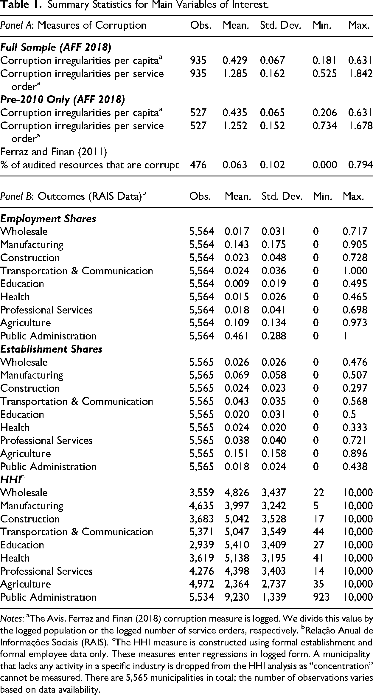
Summary statistics for these corruption indicators are given in the top panel of Table 1. Sources and descriptions are given in
Summary Statistics for Main Variables of Interest.
Summary Statistics for Main Variables of Interest.
Notes: aThe Avis, Ferraz and Finan (2018) corruption measure is logged. We divide this value by the logged population or the logged number of service orders, respectively. bRelação Anual de Informações Sociais (RAIS). cThe HHI measure is constructed using formal establishment and formal employee data only. These measures enter regressions in logged form. A municipality that lacks any activity in a specific industry is dropped from the HHI analysis as “concentration” cannot be measured. There are 5,565 municipalities in total; the number of observations varies based on data availability.
Our outcome measures come from the Relação Anual de Informações Sociais (RAIS) database for the year 2010.
27
This is a universal database of formal firms and formal employment (i.e., registered with a tax identifier). Our first aim is to test whether corruption, as defined above, impacts sectoral shares in terms of employment and establishments. To do so, we categorize establishments into eight good/service producing sectors: wholesale, manufacturing, construction, transportation and communication, health, education, professional services, and agriculture.
28
We also examine public administration. Our sector categories are defined according to the Classificação Nacional de Atividades Econômicas 2.0 (CNAE 2.0). The activities included in these sectoral definitions are given in
Focusing on the eight goods/services producing sectors first (i.e., all sectors except for public administration), we see that manufacturing comprises the largest share of total employment with approximately 14% (on average). Agriculture is the second largest (11%). The remaining six sectors only comprise between 1–2% of total employment each. However, these numbers have enormous variance—often more than double their mean value. For example, only 2.3% of total employment can be attributed to activities in the construction sector on average. But the minimum value attributed to construction is 0% whereas the maximum is nearly 73%. Moreover, the standard deviation is more than double the mean (at 4.8%). Thus, despite the seemingly low mean values, there is substantial variance in these shares across municipalities.
It is also important to note that while the sum of the first eight employment share means listed in Table 1 only sum to approximately 36% of total employment, these sectors capture most good/service producing activity. Over 50% of municipalities have a population of less than 11,000; 25% have a population of approximately 5,200 or smaller. In these small municipalities, most employment comes from public administration jobs (greater than 50%); the average employment share across all municipalities in public administration is 46% (see Table 1). Activities in this sector include social security, defense, and other government administrative activities—not the sectoral activities that we are interested in. In this sense, the 36% of total employment across the first eight sectors is capturing nearly 70% of non-administrative activities.
Establishment shares across the first eight sectors sum to only 40% of the total. Public administration accounts for approximately 2% on average. Thus, while these nine sectors capture most employment, they do not account for most establishments in a given area. This implies that the existing establishments in these nine sectors tend to be large, while establishments in the vast majority of the excluded sectors (e.g., retail and accommodations) are small. Indeed, this fits with the idea the corruption prone sectors tend to be more concentrated because monopolized industries have more rents available for extraction. This also suggests that even small changes in the share of establishments can signify large resource flows.
Lastly, we construct an HHI measure of concentration, using employment shares in place of the traditional market shares. In other words, for each sector and for each municipality, we construct the following HHI measure: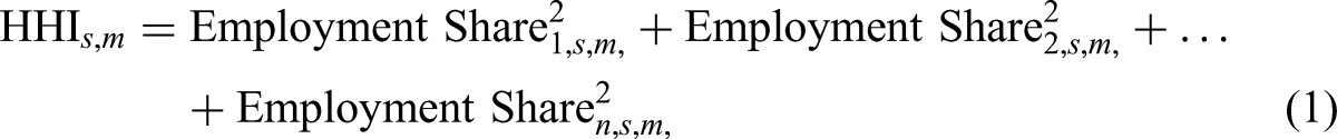
Our covariates aim to capture broad features of the local economic environment that plausibly affect both sectoral composition and within-sector concentration and are likely correlated with corruption. Although the mechanisms governing composition (e.g., sectoral choice by firms and workers) and concentration (e.g., entry, exit, and competitive structure) may differ, both outcomes are shaped by underlying levels of economic development, demographic structure, and labor market conditions. Given the close link between corruption and these factors (see, e.g., Dollar, Fisman and Gatti 2001; Torgler and Valev 2006; Dreher and Schneider 2010; Pavlik, Grier and Grier 2023; Bastos and Bologna Pavlik 2025), we view them as the most important potential confounders in our cross-sectional setting. For this reason, we use a common baseline set of covariates across specifications.
To be specific, our covariates include per capita income, population density, and the size of the informal sector (measured as a share of employment). We also control for demographic composition—the shares of the population that are working age (18–65), young (10–17), and male—as well as human capital, measured by the shares of adults (age 25+) who have completed high school and college. (Summary statistics are reported in Table 2, with variable definitions and sources provided in Table A2.)
Summary Statistics for Covariates.
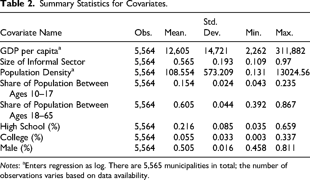
Summary Statistics for Covariates.
Notes: aEnters regression as log. There are 5,565 municipalities in total; the number of observations varies based on data availability.
In addition to the corruption indicators, the Avis, Ferraz and Finan (2018) and Ferraz and Finan (2011) studies both construct measures of general mismanagement. These acts of mismanagement are different from corruption in that they are based on irregularities associated with administrative or procedural concerns. This could involve, for example, the improper filing of documents. While this could involve corruption, it is much less egregious in nature. Our baseline estimates do not include mismanagement as a control as it is plausible to think that corruption can lead to more mismanagement, making mismanagement a “bad control” (Angrist and Pischke 2009). But we do include this variable as a control in robustness estimates presented in
Results
Baseline Results
Our baseline regressions are estimated using OLS. Our focus is on the effect of corruption on sectoral composition, and we believe this is best captured with our measure of corruption per capita. Nevertheless, for each outcome group (employment shares in Table 3; establishment shares in Table 4; and concentration in Table 5) we present estimates for three different measures of corruption. 29 We also present results both without and with the controls discussed in Section Baseline Covariates; all results include state and lottery fixed effects. Panel A of each table presents estimates without controls; Panel B presents estimates with controls. Lastly, as discussed above, because the number of service or inspection orders are not constant across audited municipalities, we additionally include a control for the number of inspections when corruption per capita is our corruption measure. The number and/or value of resources audited is implicitly captured in the corruption measures used in the other two measures and therefore is unnecessary as a control.
The Effect of Corruption on Employment Shares.
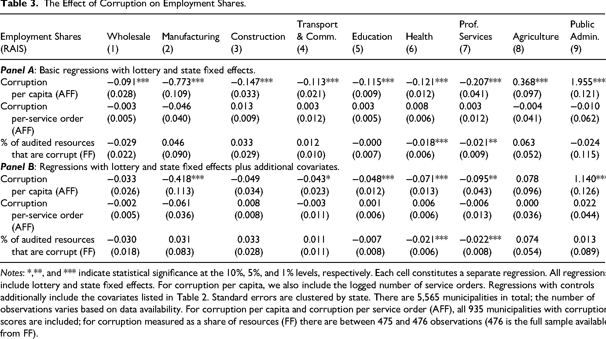
The Effect of Corruption on Employment Shares.
Notes: *,**, and *** indicate statistical significance at the 10%, 5%, and 1% levels, respectively. Each cell constitutes a separate regression. All regressions include lottery and state fixed effects. For corruption per capita, we also include the logged number of service orders. Regressions with controls additionally include the covariates listed in Table 2. Standard errors are clustered by state. There are 5,565 municipalities in total; the number of observations varies based on data availability. For corruption per capita and corruption per service order (AFF), all 935 municipalities with corruption scores are included; for corruption measured as a share of resources (FF) there are between 475 and 476 observations (476 is the full sample available from FF).
The Effect of Corruption on Establishment Shares.
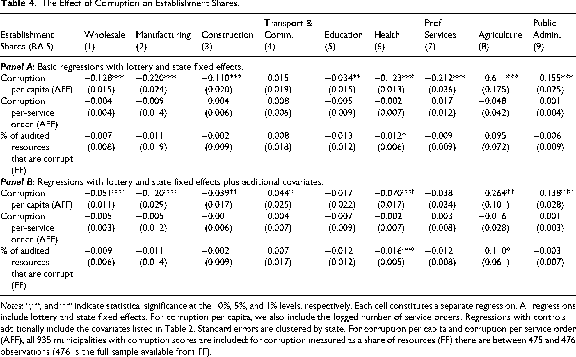
Notes: *,**, and *** indicate statistical significance at the 10%, 5%, and 1% levels, respectively. Each cell constitutes a separate regression. All regressions include lottery and state fixed effects. For corruption per capita, we also include the logged number of service orders. Regressions with controls additionally include the covariates listed in Table 2. Standard errors are clustered by state. For corruption per capita and corruption per service order (AFF), all 935 municipalities with corruption scores are included; for corruption measured as a share of resources (FF) there are between 475 and 476 observations (476 is the full sample available from FF).
The Effect of Corruption on (Logged) HHI Measure of Concentration.
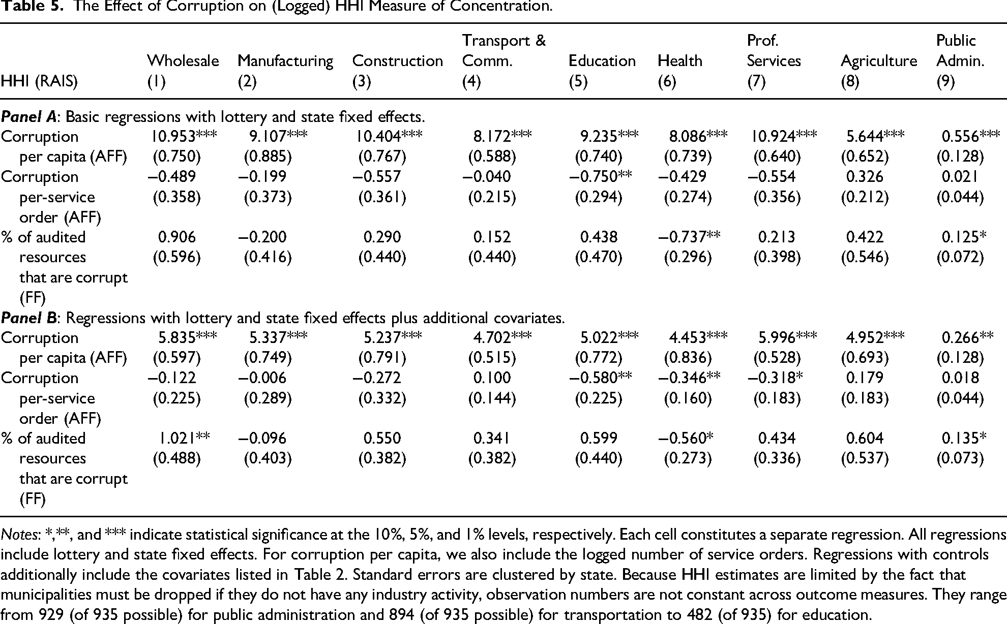
Notes: *,**, and *** indicate statistical significance at the 10%, 5%, and 1% levels, respectively. Each cell constitutes a separate regression. All regressions include lottery and state fixed effects. For corruption per capita, we also include the logged number of service orders. Regressions with controls additionally include the covariates listed in Table 2. Standard errors are clustered by state. Because HHI estimates are limited by the fact that municipalities must be dropped if they do not have any industry activity, observation numbers are not constant across outcome measures. They range from 929 (of 935 possible) for public administration and 894 (of 935 possible) for transportation to 482 (of 935) for education.
Starting with employment shares (Table 3), we find that corruption irregularities per capita are a negative predictor of employment shares in seven of the eight good/service producing sectors. Only in agriculture do we find that employment share is higher in more corrupt areas. We also find that the public administration sector is larger in more corrupt areas. All nine of these coefficients are statistically significant at the 1% level for corruption per capita in Panel A—regressions with state and lottery/audit fixed effects, along with a service order control. While we lose some statistical significance after controlling for the general level of development within each municipality in Panel B, this pattern is relatively robust in that five sectors (manufacturing, transportation & communications, education, health, and professional services) still see a significant decline in their employment shares due to corruption. These results are relatively modest in size—a standard deviation increase in corruption is associated with an 8% (transportation & communication) to 18% (health) of a standard deviation decrease in the employment shares of those five sectors. These results suggest that corruption is driving resources away from corruption prone sectors. They also seem to be driving resources towards public administration and potentially the less-corrupt sector of agriculture, though this latter result is not as robust.
Moving to the other two measures of corruption in Table 3, where corruption irregularities are scaled by the number or value of audited items, we see little association between corruption and employment shares. The exceptions are professional services and health care. In both cases, corruption is associated with smaller employment shares in these two sectors, aligning with the results above. Nevertheless, as we will also see through the remainder of the baseline results, these alternative corruption measures highlight the importance of considering population size. While we still present these results in Tables 4 (establishment shares) and
For establishment shares (Table 4), our results echo those above. There is a reduction in establishment shares across most sectors, agriculture and public administration are again the exception. The share of establishments in the transportation and communication sector also seems to increase, but this effect is only statistically significant in Panel B for corruption per capita– estimates with controls. Again, there is little in terms of statistical significance when scaling corruption irregularities by the number or value of audited items. Yet the significant results for corruption per capita seem to imply that corruption drives resources, whether this is measured as employment or establishments, away from most good/service producing sectors and towards the “safe” sector of agriculture and the administrative sector of the government. The latter is suggestive of bureaucratic bloat.
While these share results are important tests of sectoral composition, it is important to understand whether resources are underutilized in general. Despite finding that both employment shares and establishment shares decline across industries in corrupt areas, we need a more precise estimate of concentration. To do so, we estimate corruption's effect on our HHI measure discussed above. These results are presented in Table 6 and yield our most striking result. We find that corruption per capita is associated with increased concentration across all nine sectors. While the magnitude of the coefficient shrinks when we include our baseline set of controls, every coefficient remains statistically significant at the 1% level or better for eight of the nine sectors. For the ninth sector (public administration), the coefficient is statistically significant at the 5% level. Even using these smaller sets of coefficients, we find the corruption has a meaningful effect on concentration. For example, for the goods/service producing sectors, a standard deviation increase in corruption per capita results in anywhere from a 30% increase in firm concentration (health) to a 40% increase (professional services). Corruption even increases the concentration of the public administrative sector by 1.78%. While seemingly small, this is a relatively important effect given that most public administration sectors are heavily concentrated to begin with. 30 As above, the results are generally insignificant or inconsistent for the alternative corruption measures.
The Effect of Corruption per Capita on (Logged) HHI Measure of Concentration (Outcomes in Listed in
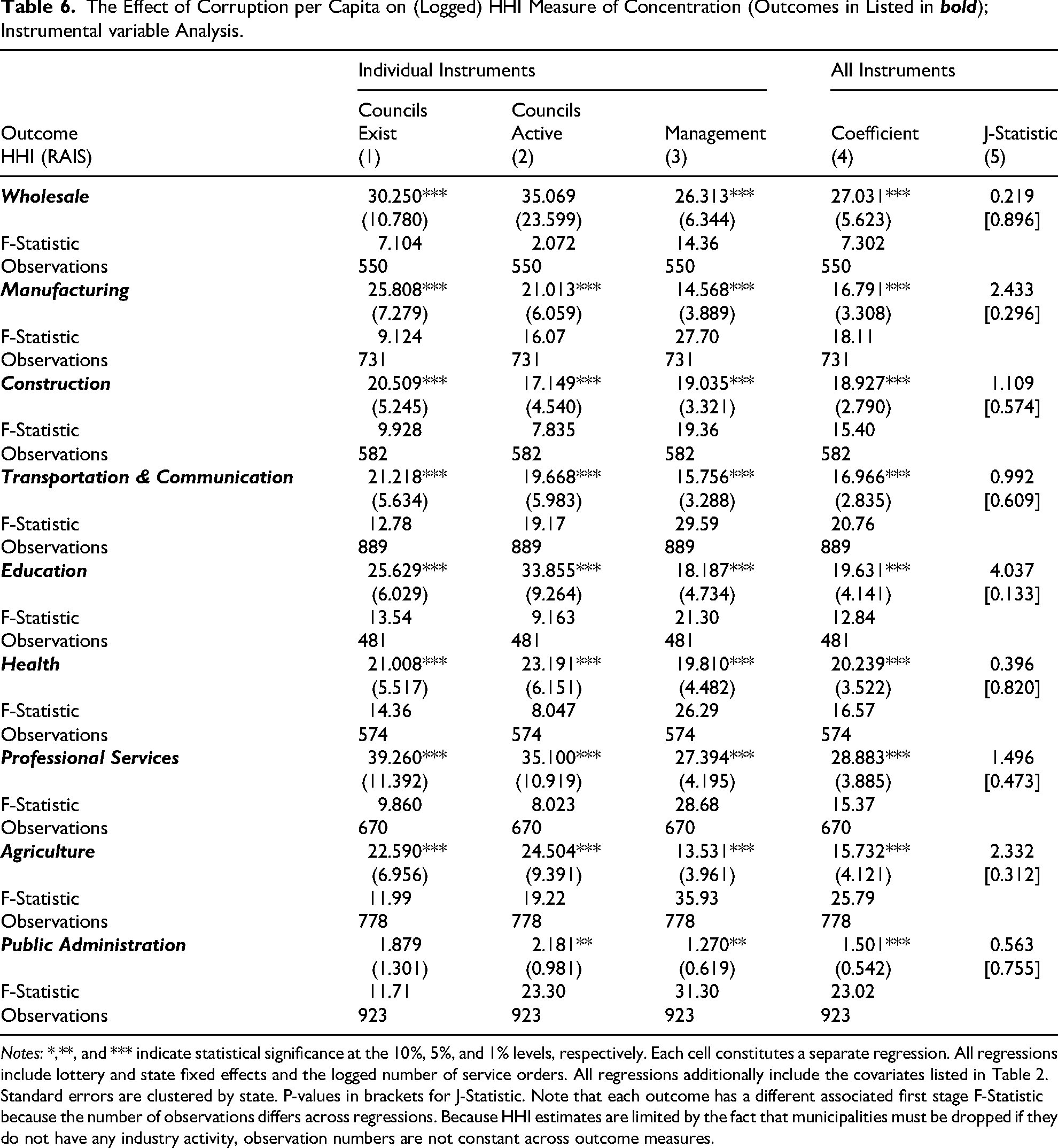
Notes: *,**, and *** indicate statistical significance at the 10%, 5%, and 1% levels, respectively. Each cell constitutes a separate regression. All regressions include lottery and state fixed effects and the logged number of service orders. All regressions additionally include the covariates listed in Table 2. Standard errors are clustered by state. P-values in brackets for J-Statistic. Note that each outcome has a different associated first stage F-Statistic because the number of observations differs across regressions. Because HHI estimates are limited by the fact that municipalities must be dropped if they do not have any industry activity, observation numbers are not constant across outcome measures.
An obvious concern with our analysis, and most analyses involving estimating the effects of corruption, is the presumed exogeneity of corruption per capita. Determinants of corruption are far ranging, and the overlap of corruption causes with causes of business activity is certainly plausible. We attempt to control for some of this using general municipal indicators for development in our baseline regressions and by always including state fixed effects. Nevertheless, this concern is legitimate.
In the absence of a randomized experiment, one potential solution to this endogeneity problem is the use of instrumental variables. While useful in theory, it is well-known that the problems of instruments can outweigh their benefits if their two conditions are not met: (1) instrument validity and (2) instrument exogeneity. In other words, we need to identify factors that are strongly correlated with corruption but are otherwise uncorrelated with our outcomes of interest. We propose three potential variables for this purpose: the existence of local councils, the activity of local councils, and management capacity. We believe all three are strongly correlated with corruption—condition number one. We also have reason to be believe that they are plausibly exogenous. However, given that we can never prove exogeneity, we intend these results to only be used as a robustness check.
The existence and activity of local councils is a proxy for political competition and/or local accountability. 31 These measures come from a 1998 index constructed by the Instituto Brasileiro de Geografia e Estatística (IBGE) aiming to capture the institutional quality of each municipality (Indicador de Qualidade Institucional Municipal—IQIM). The existence indicator simply counts the number of municipal councils in existence and puts this value into a 1 (least councils) to 6 (most councils) index scale. The activity of local councils is similar but additionally considers if these councils were active in the sense that they had individuals appointed in positions. Municipalities with more local engagement in government is likely to have less corruption.
The management capacity indicator also comes from this same IQIM index. This measure examines whether the municipality has implemented districts or administrative regions (decentralized management), zoning plans and/or laws, building codes, and codes of conduct that establish fines for littering, licensures, operating hours, and more. The presence of such plans/laws signifies that the municipality has the capacity to implement them. We thus interpret this measure as a predictor of state capacity. While the correlation between state capacity is theoretically ambiguous (i.e., is a stronger state less corrupt?), this measure is specific enough to proxy for the ability of a municipality to carry out complex tasks. One such task might be corruption monitoring. Indeed, the raw correlation between this measure and corruption per capita is strongly negative at −0.42.
Because all three instruments are measured in 1998, this rules out the concern of reverse causality. Yet dual causality remains a concern. It is easier to argue for the plausible exogeneity of the first two instruments—the existence and activity of local councils. Local councils act as a check on corrupt behavior and impact business only through their effect on corruption. Management capacity is more of a concern as some sectors are likely more sensitive to rules/regulations than others. This is a concern for our share outcomes in that municipalities with more rules that affect a particular sector could reduce that sector's share of activity. Similarly, rules/regulations could directly impact concentration. Yet, this indicator is the strongest predictor of corruption. We therefore proceed carefully as follows.
First, we present and focus our IV results for each instrument separately: council existence, council activity, and management. We then include all three instruments together and estimate the appropriate J-Statistic, allowing us to test whether there is any evidence that our instruments are not exogenous (Table 6). Second, we repeat this analysis but additionally include a control for mismanagement. The audits not only revealed malfeasance in the form of corruption but also included less nefarious acts of mismanagement. In this way, we can test whether corruption is still an important predictor after controlling for general inefficiencies in management. (We also include this mismanagement control in all baseline (non-instrumental variable) regressions in
For brevity, our focus in this section is on the robustness of Table 5, results with HHI as our outcome, as this is our strongest result.
32
For all instrumental variable analyses, we only focus on corruption per capita. Table 6 presents the set of results where we instrument for corruption with the existence of councils, appointment of councils, and management capacity—all separately in columns 1 through 3. And then include all three instruments together (column 4). As shown in the table, management capacity is by far the strongest instrument. This is also confirmed in the first stage estimates presented in
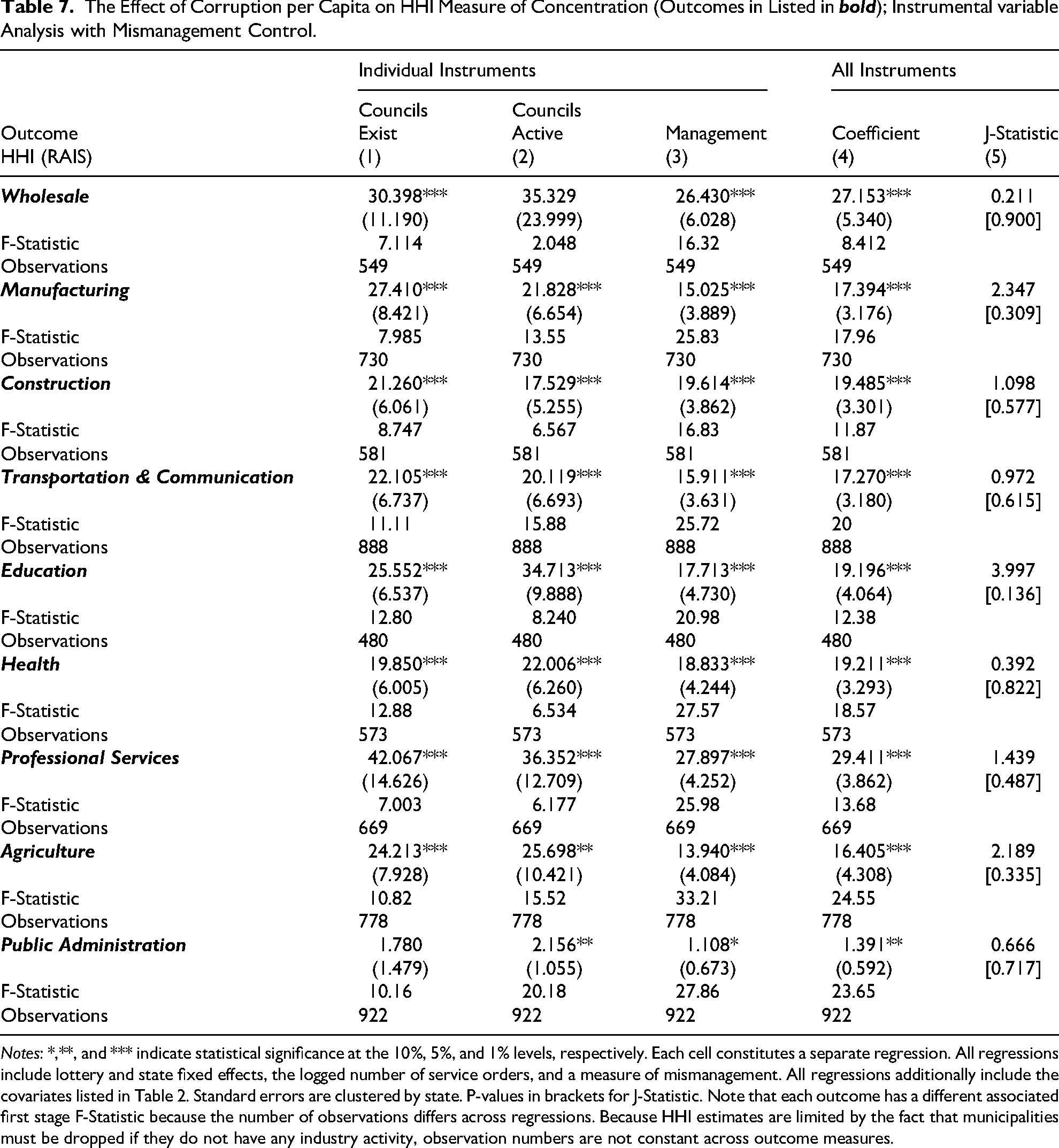
The J-Statistic in column 4 of Table 6 is never significant, suggesting that our instruments are potentially exogenous. But the null of the J-Statistic is that the instruments are exogenous. Thus, a p-value of 0.15, for example, would suggest that there is an 85% change of endogeneity, which is not reassuring. We therefore conduct several robustness checks. Our primary one, given in Table 7, is to additionally include the mismanagement control. The results are again robust and consistent across the four estimates. But here, the J-Statistic is generally much smaller, implying that endogeneity is less of concern.
The Effect of Corruption per Capita on HHI Measure of Concentration (Outcomes in Listed in
bold
); Instrumental variable Analysis with Mismanagement Control.
The Effect of Corruption per Capita on HHI Measure of Concentration (Outcomes in Listed in
Notes: *,**, and *** indicate statistical significance at the 10%, 5%, and 1% levels, respectively. Each cell constitutes a separate regression. All regressions include lottery and state fixed effects, the logged number of service orders, and a measure of mismanagement. All regressions additionally include the covariates listed in Table 2. Standard errors are clustered by state. P-values in brackets for J-Statistic. Note that each outcome has a different associated first stage F-Statistic because the number of observations differs across regressions. Because HHI estimates are limited by the fact that municipalities must be dropped if they do not have any industry activity, observation numbers are not constant across outcome measures.
Lastly, we replace the management instrument with the distance to the federal capital estimate. These results are available in Table 8. One glaringly obvious concern with this set of instruments is that they are relatively weak as a set. In addition, the J-Statistics are relatively large compared to the previous estimates. Nevertheless, again, the coefficients are all positive and statistically significant though these latter results should be interpreted with caution.
The Effect of Corruption Per Capita on HHI Measure of Concentration (Outcomes in Listed in
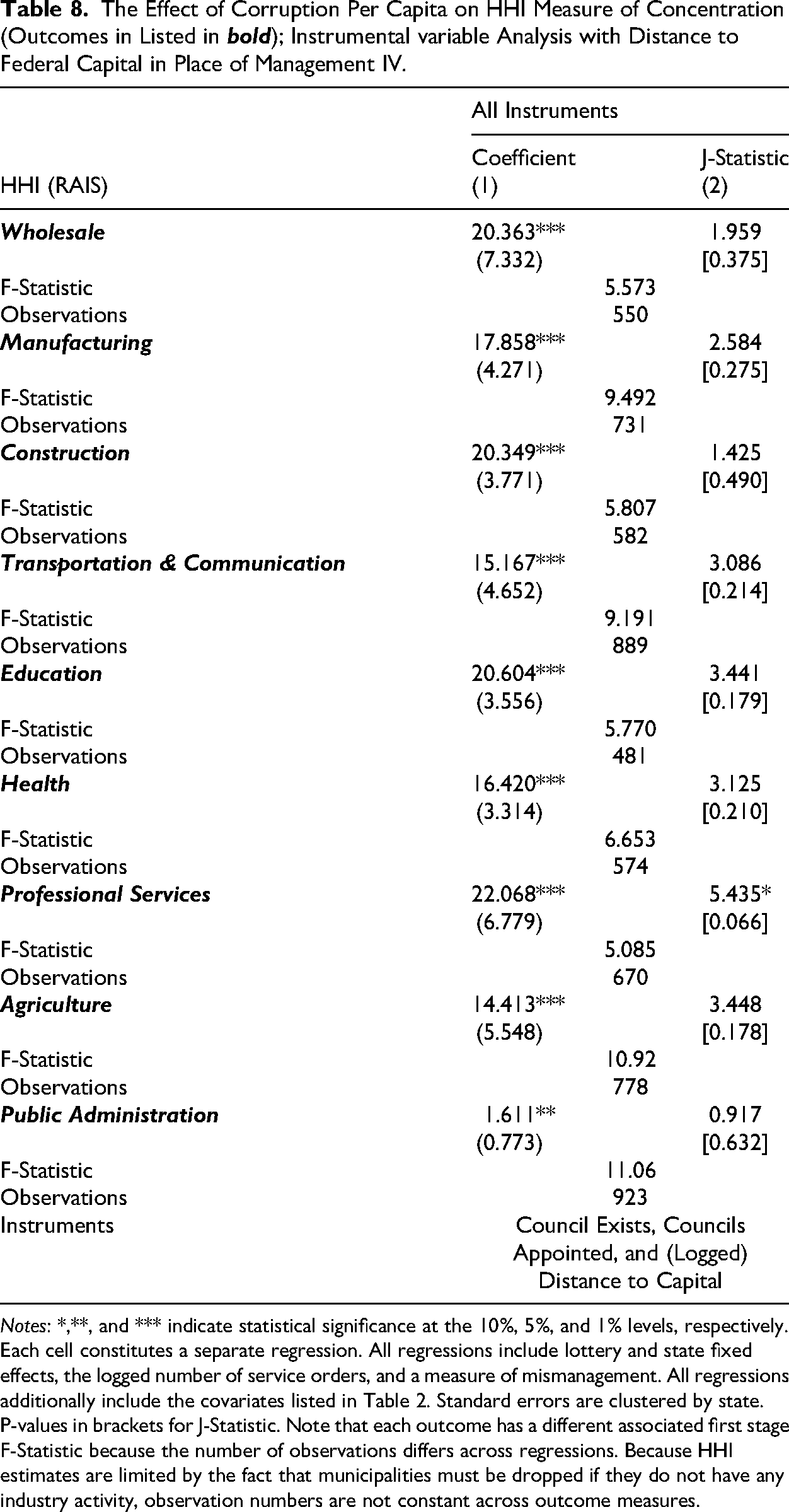
Notes: *,**, and *** indicate statistical significance at the 10%, 5%, and 1% levels, respectively. Each cell constitutes a separate regression. All regressions include lottery and state fixed effects, the logged number of service orders, and a measure of mismanagement. All regressions additionally include the covariates listed in Table 2. Standard errors are clustered by state. P-values in brackets for J-Statistic. Note that each outcome has a different associated first stage F-Statistic because the number of observations differs across regressions. Because HHI estimates are limited by the fact that municipalities must be dropped if they do not have any industry activity, observation numbers are not constant across outcome measures.
The idea that corruption is harmful to business activity is well-known. Much of the work looks at the impact of corruption on aggregate levels of output (e.g., number of establishments, incomes, overall GDP per capita). Except for Boudreaux, Nikolaev and Holcombe (2018), little work has examined this effect at a cross-industry level. In this study, we find that corruption is associated with a reduction in employment and establishment shares in most industries except for agriculture (which is typically seen as less corrupt) and the public administration sector (suggesting an increase in government size and scope).
These findings contrast with that of Boudreaux, Nikolaev and Holcombe (2018), who show that corruption increases establishment shares of more corrupt sectors like construction. While this difference is potentially puzzling, we note two key differences between our studies. First, our measure of corruption is different than that of Boudreaux, Nikolaev and Holcombe (2018). We use a measure of corruption that stems from random audits, while the aforementioned study uses federal corruption convictions. Their measure relies on the ability of the legal system to successfully identity and prosecute corruption, which may be easier to do in areas like construction. We use a broader measure from Avis, Ferraz and Finan (2018) that is less susceptible to legal system quality. Second, they examine the effect within the United States, which is a richer country than Brazil. In high income countries, Dreher and Schneider (2010) argue that bribes are less coercive and more likely to be the consequence of rent seeking and opportunistic behavior on part of the private sector actors. Given Brazil's differing economic performance and political institutions, it is not unexpected that engaging in bribes can be seen as a riskier endeavor, as it is less likely that the bribe would be binding. As such, we would expect individuals to stay away from corrupt sectors in Brazil (relative to the United States).
Perhaps most interestingly, we also find that corruption increases industry concentration within every industry, including those both those are seen as largely corrupt and those that are less so. These results hold under a variety of robustness tests, including: an instrumental variable analysis, controlling for mismanagement, and alternative samples/measures. These findings are complementary to the corruption-inequality literature, which generally shows that higher levels of corruption increase the concentration of wealth and income to a small group of elites. They are also suggestive of an entry limiting effect. Corruption seems to make all sectors more concentrated, leaving less room for entrepreneurs to thrive. Taken together, our results suggest that productive entrepreneurs are avoiding corrupt sectors and are potentially limited in number due a concentration effect.
Our findings reveal interesting policy ramifications. Ferraz and Finan (2008) show that findings from the audit programs had an influence on the incumbent mayor's reelection outcomes, and Avis, Ferraz and Finan (2018) find that corruption levels drop by 8% after the audit programs. These accountability mechanisms reveal that the audit programs themselves had an influence on outcomes. Taking our results seriously suggest that addressing corruption in a meaningful way can allow for a higher dispersion of firms, which can raise wages according to the monopsony model. Furthermore, a less concentrated sector environment allows individuals to select into industries based on skillsets and comparative advantages, as opposed to avoiding certain industries because of corruption.
Further, we believe there are several interesting future avenues of research that could build off our result. First, one could examine how corruption shapes the share of production going towards workers/labor; Young and Lawson (2014) find that capitalistic institutions are associated with greater levels of labor share. Second, given data availability, it would also be interesting to develop more robust measures of productive entrepreneurial activity along the lines of Sobel (2008) to test whether creative activity is indeed diminished in corrupt municipalities. Third, given that Brazil is a federation, one could also explore how local corruption interacts with national regulations in its effect on local business activity. Lucas and Boudreaux (2020) study a similar dynamic in national regulation versus state-level policies within the U.S. Lastly, our study focuses on sectoral composition and market structure, a related study could also explore how these corruption effects limit agglomeration benefits, i.e., the benefits of concentrating specific types of economic activities within a specific locale.
Supplemental Material
sj-pdf-1-pfr-10.1177_10911421261456494 - Supplemental material for Corruption and the Composition of Business Activity in Brazil
Supplemental material, sj-pdf-1-pfr-10.1177_10911421261456494 for Corruption and the Composition of Business Activity in Brazil by João Pedro Bastos, Justin T. Callais and Jamie Bologna Pavlik in Public Finance Review
Footnotes
Funding
The authors received no financial support for the research, authorship, and/or publication of this article.
Declaration of Conflicting Interests
The authors declared no potential conflicts of interest with respect to the research, authorship, and/or publication of this article.
Supplemental Material
Supplemental material for this article is available online.
Notes
Author Biographies
References
Supplementary Material
Please find the following supplemental material available below.
For Open Access articles published under a Creative Commons License, all supplemental material carries the same license as the article it is associated with.
For non-Open Access articles published, all supplemental material carries a non-exclusive license, and permission requests for re-use of supplemental material or any part of supplemental material shall be sent directly to the copyright owner as specified in the copyright notice associated with the article.