Fast GPU perspective grid construction and triangle tracing for exhaustive ray tracing of highly coherent rays

Abstract

In this article, we address the problem of computing, storing and sorting, at an interactive rate, all of the intersections between millions of triangles (a 3D scene) and millions of rays starting from the same point. In this paper we focus on the fast GPU construction of a grid in projective space referencing the triangles of a 3D scene. We introduce a fast GPU algorithm used to build a grid of the rays constituting the scene, in the same projective space. This ray-based grid is computed during the initialization of the scene, which allows us to achieve higher performance, and to construct the triangle-based grid in distinct passes for very large scenes, without having to manage memory transfers between CPU and GPU. This algorithm works the same way for both static and dynamic scenes, allowing us to achieve interactive processing of complex and dynamic scenes. These optimizations are used to speed up the geometrical computations used in the nuclear field to evaluate the impact of radiative sources on an operator. These geometrical computations are similar to those of traditional ray tracing, except that only highly coherent rays are thrown in our application, and that we are looking for all intersections along each ray.

Keywords

dosimetry GPU grid construction radiation protection raytracing

1 Introduction

Preparing interventions in the nuclear field notably implies an evaluation of the impact of radiative sources on operators. Numerous computation codes exist to simulate the propagation of radiations, but most of them operate offline. In addition, decreasing computation times in a noticeable way brings interactivity to the user, allowing him to interact with the scene and to intuitively study more appropriate scenarios. For radiation protection purposes, people often take advantage of simplified methods and algorithms, such as the straight-line attenuation method with build-up factors (Assad et al. 1999), which, in most cases, gives results of the same order of magnitude as those produced with more exact methods. In this method, the radiative sources are represented as groups of punctual sources. To compute the radiations received at a given position, rays are traced between this point and the sources. For each ray, all of the intersections with the objects of the scene must be found (see Figure 1 ). Since the treated scenes can have millions of triangles, a very high number of intersections will have to be stored. Even if additional computations are necessary before getting a final result, the bottleneck of the overall simulation always remains in these ray tracing requests.

Figure 1.

NuclearCase scene (738,000 triangles) from two different points of view. A total of 600,000 rays are traced, for 6 million intersections sorted, in 250 ms on a NVIDIA GTX 295. Rays are colored in white and become red when meeting an object.

Two main differences appear between our approach and traditional ray tracing. First of all, this approach does not require the management of secondary (and incoherent) rays. On the other hand, however, the primary rays of the approach are similar to those of ray tracing: coherent rays, all starting from the same point. The second main difference between the two approaches is that all intersections along each ray have to be stored. This requirement, absent of usual ray tracing, is very demanding, as explained later. Moreover, these intersections also have to be sorted, in order to compute depths of material intersected along each ray. These depths will be used as inputs to compute the radiations received at one point.

The paper is organized as follows: in the next section, we review previous work on ray tracing and rasterization. We then present the classical ray-tracing algorithm, and explain why we decided to switch the first two steps of this algorithm to solve our problem (Section 3). Section 4 consists of a detailed description of the grid construction algorithm. The exhaustive triangle-tracing algorithm is also described in Section 5. Finally, we present our results in Section 6, then conclude and present directions for future work.

2 Background

2.1 Ray tracing

The problem of computing intersections between coherent rays and triangles has been investigated a lot. Real-time ray tracing, achieved during the last decade, owes its existence greatly to the use of algorithms performing extremely well for coherent rays, including the introduction of ray packets (Wald 2004). Coupled with fully optimized kd-trees (Reshetov et al. 2005), algorithms specially optimized for coherent rays have brought impressive performances.

For several years, the Bounding Volume Hierarchy (BVH) has become the best solution for most coherent rays (Wald et al. 2007), such as primary rays Cadet and Lecussan (2007), because it enables the traversal of very large packets. However, in the extreme case where all of the rays start from the same point, kd-tree or BVH are not the best structures anymore. Hunt and Mark (2008) defined a grid in perspective space (see Figure 2 ) that turns out to be the most appropriate structure for primary rays. The special shape of this grid allows a great reduction of the traversal time for each ray, compared with the ones you can get with kd-trees or BVHs.

Figure 2.

Example of two triangles A and B in a perspective view. The associated perspective grid has a resolution of 4 * 4, indices of the cells are indicated in the upper-left corner of each cell. Red circles numbered from 0 to 9 are the rays starting from the eye.

To deal with dynamic scenes, the acceleration structures have to be updated for each frame of the scene. It is possible to only update some nodes of the tree for BVHs (Lauterbach et al. 2006), but it does not work for all kinds of dynamic scenes, and can lead to trees of very bad quality after some number of frames. Interesting attempts exist to update the BVH, and asynchronously rebuild another BVH concurrently to use the new one after some number of frames (Ize et al. 2007).

In terms of construction times, great performances have been achieved for BVHs (Lauterbach et al. 2009) and kd-trees (Zhou et al. 2008), but they are still clearly outperformed by those obtained for grids (Kalojanov and Slusallek 2009). The major drawback of the perspective grid is that it has to be constructed for each frame, for both static and dynamic scenes. However, thanks to the obtained construction times, this grid still outperforms other approaches for primary rays (Hunt and Mark 2008). In this way, this drawback can become an advantage, since the dynamic and static scenes are treated in the same way.

2.2 Rasterization

As noted by Hunt and Mark (2008), the perspective grid has many similarities to a Z-buffer. In our case, ray coordinates are known in advance, as in traditional rendering. Therefore, it is natural to try to use the works of the rendering community to solve our problem. Most of the time, to render a 3D scene, triangles are streamed through the graphic pipeline, and the first intersection along each ray (here a pixel of the screen) is kept thanks to the Z-buffer (Catmull 1974). If very high framerates can be obtained with rasterization techniques, they are not applicable to the storage of all of the intersections for each pixel. As a matter of fact, in the rasterization approach, the amount of memory available for each pixel is constant, and limited, so that other ideas have to be found to solve our problem.

In fact, the problem of taking into account every intersection has also received much attention, since it can be essential to solve aliasing problems, or to render transparency effects. The first way to solve this problem is to modify the hardware, and hence modify the storing of the results: the first proposition of such a system was the A-buffer (Carpenter 1984), in which all fragments were stored as linked lists. Other solutions have been proposed more recently (Jouppi and Chang 1999; Wittenbrink 2001), and an implementation of the F-buffer (Mark and Proudfoot 2001) has been made available (Houston et al. 2005), but was restricted to ATI’s graphics hardware.

Other solutions have to be found, since hardware modifications are not an option in this case. The most intuitive may be depth-peeling (Everitt 2001): in each rasterization pass, the first intersection is stored. Hence, a first pass can be executed, to store the results, and then a new pass can be executed adding a depth test taking into account the results of the previous pass. By repeating this process n times, the n first intersections can be stored for each ray. However, since all intersections have to be stored, the maximum number of intersections for one ray can be very high. The number of passes needed would be equal to the maximum number of intersections for a ray of the scene. This would lead to a number of passes that is very difficult to predict, and potentially very high.

The same problem exists with the k-buffer (Bavoil et al. 2007), which allows us to store k intersections by pixel. This technique begins to be less efficient for k = 8, which would again force us to run multiple passes. In order to treat all intersections, the k-buffer technique performs blending operations between fragments, which cannot be used in our case. Moreover, the k-buffer suffers from read–modify–write (RMW) hazards, and the solutions found strongly decrease performance level. These RMW hazards no longer exist with the depth-peeling improvement proposed by Liu et al. (2009): as for the k-buffer, multiple render targets (MRT) buffers are used to store up to 32 intersections for each pixel. However, with this solution, intersections too close to each other can be missed. Such a limitation cannot be accepted in our application case.

To sum up, none of the existing techniques completely solves our problem. Another problem comes from the fact that the rasterizer can only be used for regularly spaced rays. In our application, all rays share the same starting point, but the spacing between each other can be completely irregular. Irregular rasterizers have already been proposed (Johnson et al. 2005; Aila and Laine 2004), but they also require a modification of the hardware.

3 Algorithm presentation

The structure that is used here is the perspective grid, since it is the best structure for rays that share the same starting point and since its construction time can be really low. Since all of the intersections have to be found along each ray, the 2D version of this perspective grid has been implemented. In addition, high-level GPU programming languages, such as CUDA (NVIDIA 2009) and OpenCL (OpenCL 2009), have greatly simplified the programming on the GPU. It is now simple to perform efficient sort (Merrill and Grimshaw 2010; Satish et al. 2009), scan (Sengupta et al. 2007) and stream compaction (Billeter et al. 2009) operations. Thanks to this, the construction of the grid and the computing of all of the intersections can be done on the GPU.

The GPU grid construction algorithm we present here has strong similarities with those proposed by Kalojanov and Slusallek (2009) and Ivson et al. 2009. However, our implementation is optimized for the computation of every intersection, and our algorithms allow us to avoid the grid storage issues mentioned by Kalojanov and Slusallek (2009).

After having chosen the grid in projective space as an acceleration structure, a classical approach would be:

build a grid giving, for each cell, the list of triangles it overlaps;

then, for each ray, find the corresponding cell, and, thanks to the grid, find the corresponding triangles with which intersections need to be tested;

finally, compute the intersections between rays and triangles.

We explain in this section why we decided to change the structure of the algorithm, build a ray grid, and create partial triangle grids.

3.1 Grid storage issue

First comes a description of the data organization chosen to represent the grid, identical to that presented by Lagae and Dutré (2008). Working on the GPU, it is not possible to have for each 2D cell a vector giving the indices of the triangles intersecting the cell, as the access to these vectors from the GPU kernel would be tedious. Instead, a unique vector, called trgIds, is used. It stores contiguously the indices of triangles overlapping each cell. These indices are sorted by the index of the corresponding cell.

Now, given a cell i, it is necessary to know how to obtain the list of triangles overlapping this cell. This piece of information is given by a second vector, cellStartId. cellStartId[i] gives the position in trgIds where the list of triangles that correspond to the cell i begins. In this way, indices of triangles overlapping a given cell i will be found in the vector trgIds, between the positions cellStartId[i] and cellStartId[i + 1]. The construction of the grid thereby consists of the construction of these two vectors, obviously as fast as possible.

The main concern with this approach comes from the size of these two vectors, which can vary significantly from one scene to another, or even from one viewpoint to another, and cannot be directly predicted knowing only the number of triangles in the scene. Scenes with numerous large triangles are likely to be difficult to handle. The Sully Scene (804,000 triangles) is a good example of such a scene. The grid of this scene is composed of more than 10 million cells, which means that after the only building of the grid, and before any intersection test is made, a lot of memory is already used on the graphical unit to store ray and point coordinates, triangle descriptions, and these two vectors.

3.2 Triangle tracing

Here we describe why we decided not to construct this grid, and swap the steps 1 and 2 of the algorithm described at the beginning of this section. Instead of what was presented, we build a grid that stores information about rays. This grid enables us to know, for each cell, which rays fall inside of it. The building of this new ray-oriented grid will be the new initialization step of the algorithm. Then, during the computation step, triangles will be ‘traced’ against the ray grid: for each triangle, the cells overlapping the triangle are found, and then intersections are computed with rays overlapping these cells.

By doing this switch, this technique becomes practically equivalent to hierarchical rasterization, which is quite logical, since those approaches face similar problems:

Building a fixed regular grid in 2D perspective space is equivalent to a regular tiling of the screen.

Streaming over triangles, and building a grid over them, is equivalent to testing triangles against the tiles of the screen.

Intersecting rays and triangles within the same cell is equivalent to performing sample tests in screen tiles which overlap the triangle.

Generating all hits, rather than just the nearest hits: with depth testing optimizations disabled, a rasterizer will always generate all hits.

In fact, this switch basically corresponds to irregular rasterization. It can also be noted that some of the first attempts to adapt the ray-tracing algorithm on the GPU were based on a very similar idea: targeting older-generation GPUs with limited programmability, Carr et al. (2002), for instance, also streamed the triangles, testing each against all rays.

The difference with hierarchical rasterization here comes from the storing of all hits, which is made possible with our technique. Also, as stated above, a classical hardware rasterizer cannot be used if the rays are not regularly spaced.

The construction algorithm of the classical projective grid requires a radix sort on a vector which size is the number of triangle/cell pairs (noted nbRefs) that can be found in the scene. This radix sort is the bottleneck of the overall simulation. Instead, the radix sort used for the ray grid construction will be applied to a vector the size of which is the number of rays falling in a cell of the grid (denoted nbRaysUsed). Except for very small scenes, nbRaysUsed will always be far smaller than nbRefs (we need approximately a million rays in our scenes, and have found the best resolution to be 1,000 × 1,000 for the grid). This will make the radix sort far faster for most cases. The use of the ray grid will also imply sorting the intersections found by the index of the ray, but, during our tests, the ray grid always remained more efficient. The fact that the ray grid is far smaller than the triangle grid will also reduce the time needed to bind arrays to texture, which can be relevant for very large scenes.

The second main reason for doing this switch is that it is now possible to build the triangle grid in multiple passes. In this way, the memory that has been used for a previous group of triangles can be deallocated before treating another bunch of triangles. The only memory that cannot be freed between these passes is the one used to store intersections. However, this is not demanding, as an intersection is described by 8 bytes: an integer for the ray index, and a single float for the coordinate of the intersection along the ray. Hence, scenes with lots of large triangles can now be treated, and transfers to the CPU mentioned by Kalojanov and Slusallek (2009) to avoid memory overflows are no longer needed.

The last advantage of this algorithm is that it can be easily used on multi-GPU platforms, as the ray grid just has to be duplicated on each GPU, and then each GPU can handle a unique set of triangles.

4 Ray grid construction

After having exposed the reasons for introducing the ray grid, we present in this section the algorithm (see Figure 3 ) used to construct the ray grid in perspective space using the GPU. An example of a very simple scene can be seen on Figure 2. Figure 3, presenting the algorithm exposed in the next section, use this case as an example.

Figure 3.

Ray grid construction algorithm. The GPU vectors given as an example use the grid presented in Figure 2. cellStartId is of size gridSize + 1, in order to obtain the number of rays in the last cell by computing cellIdOfRay[gridSize] – cellIdOfRay[gridSize – 1].

The two vectors describing the grid are named rayIds and cellStartId, with the same conventions than with the triangle grid (See 3.1). The different steps of the algorithms can be found on the figures, they are numbered like the different subsections.

4.1 Find ray position in projective grid

First step of the algorithm is obvious: nbRay threads are launched, each one working on one ray and finding in which cell it falls.

4.2 Group rays by cellId

The next step of the algorithm consists of sorting ray/cell pairs (respectively found in rayIds and cellId Of Ray) by increasing index of the cell. In this way, the rays that belong to the same cell will be contiguous in memory. For a grid resolution of 1,024 × 1,024, only the 20 first bits are relevant for each cell index. To provide better performance, the sort algorithm used has to be able to consider 20 instead of 32 bits for the key data. We used here the sort implementation of Thrust (Hoberock and Bell 2009), based upon the latest results in the literature (Merrill and Grimshaw 2010; Satish et al. 2009), which presents this optimization.

This step is in fact the bottleneck of this ray grid construction. It can be noted that rayIds is already the vector we wanted to produce.

4.3 Count number of rays by cell

Now comes the less obvious parts of the algorithm. To construct the reference vector cellStartId describing where each cell begins in rayIds, it is first necessary to generate an array giving the number of rays each cell contains (it will be obtained at step 4.4). This array will be first initialized with zeros. Then we need the number of rays in each non-empty cell and the position where to write this number in the array, given by the index of the associated non-empty cell. On a CPU, these pieces of information are easy to find by executing a simple loop on the array cellIdOfRay generated in step 4.2. It is not possible to directly adapt this loop on the GPU, because it would produce writing conflicts. To avoid these conflicts, it is necessary to generate two separate vectors, one giving the indices of the non-empty cells, and the other giving the number of rays in each of these cells, indicating respectively where and what each thread will have to write to produce a correct array at step 4.4.

These two arrays are easily obtained by performing a segmented reduction, with cell indices (from cellIdOfRay) as keys and a constant array of ones as values. An efficient implementation of this operation can also be found in Thrust (Hoberock and Bell 2009) (see thrust::reduce_by_key).

4.4 Write number of rays by cell

Thanks to the previous step, it is now possible to write the values included in nbRaysByCell in the array cellStartId, at positions given by cellIdOfRay.

4.5 Final writings in cellStartId

Now that the number of rays in each cell is written in the array cellIdOfRay, an exclusive scan on this array provides a vector cellStartId; that is exactly what we wanted.

5 Triangle tracing

After this initialization comes the phase that could be called triangle tracing. For each triangle, the cells overlapping it are identified. Then, thanks to the ray grid, the potentially intersecting rays are found, and the intersection tests are performed.

We consider that the triangles are already projected in the 2D frame chosen. The algorithm used to build the grid is given in Figure 4 , it also refers to the Figure 2.

Figure 4.

Triangle grid construction algorithm. The GPU vectors given as an example use the grid shown in Figure 2.

The first four steps of the algorithm can be seen as a very partial construction of the triangle grid. Here, it will only be a list of the triangle/cell pairs found, when the classical algorithm would also have included a sort of these pairs by the index of the cell and other steps to generate the vector of references cellStartId. Compared with the ray grid algorithm presented in the previous section, it could be said that only the step 4.1 is executed here. However, this step is in fact more complicated and time-consuming, since each triangle can overlap more than one cell.

5.1 Prepare to store results for each line

The triangles are rasterized via a scanline algorithm. To reduce load-balancing issues that could be created by triangles of very different widths, they will be divided into different lines, and then each thread will work on a different line. Since the number of lines for each triangle cannot be known in advance, it is not possible to directly predict where each thread will have to write its own results.

Therefore, each thread is being assigned a triangle, and must count the number of lines (of the grid) it overlaps. The result is written in nbLines An exclusive scan is performed on this vector, so that each thread working on the triangle i will write its results at the position nbLines[i] in the array startStop.

5.2 Store line coordinates

The structure startStop[i] is composed of three integers, so that startStop[i].start and startStop[i].stop are, respectively, the beginning and ending indices of cells for the line number i in the overall scene. The index of the triangle concerned by this line is given by startStop[i].trgIdx.

Each thread working on a triangle now scans the lines between the highest and the lowest vertex of the triangle, and stores the startStop associated with each of these lines, beginning to write at position nbLines[i].

5.3 Prepare to store results for each cell

The same work than that executed for lines is now made for cells. First, a new kernel is run, which counts the number of cells for each line. An exclusive scan on the resulting vector provides the total number of cells, and the position where each thread working on one line will write the corresponding cell/triangle pairs.

5.4 Generate all triangle/cell pairs

Hence, a new kernel is thrown, in which each thread works on one line, and effectively stores in memory the associated triangle/cell pairs.

5.5 Prepare to store intersections

Now that the cell/triangle pairs are generated, we just have to find for each cell the rays it contains. Then, the intersection tests will be made with the associated triangle. Since each cell can contain more than one ray, it is necessary to begin by computing the number of tests to be executed for each cell. This is done by using for the first time the ray grid generated in Section 4. The number of rays falling on a cell of index i is given by the value cellStartId[i+1]−cellStartId[i]. Each thread working on a different cell/triangle pair counts the number of rays contained by its cell. This value is the number of tests that will be executed for the associated cell/triangle pair. An exclusive scan on the generated array provides the positions where each thread will have to store the indices of rays/triangles to be tested.

5.6 Fill indices of rays/triangles for intersection tests

Then, each thread is being assigned a cell/triangle pair, and, thanks to the previous step, generates the ray/triangle pairs to test.

5.7 Compute intersections

To store these results, two arrays result and rayAndCoord are created. If an intersection is found for test number i, result[i] is set to 1, and rayAndCoord[i] to the value (rayId, t), where rayId is the index of the related ray, and t the intersection coordinate. If M is the intersection point, and $\vec{O} P$ the ray, t is defined such that $\vec{O} M = t . \vec{O} P$ .

To compute the final list of intersections, elements in the array rayAndCoord unrelated with an intersection are removed. The array rayAndCoord is then sorted by increasing index of ray. Then, intersections related to a same ray are sorted by t coordinate. Therefore, rayAndCoord is then the array of intersections that had to be produced.

6 Results and discussion

6.1 Implementation

Having described the algorithms used in our GPU exhaustive raytracer, we can now evaluate its performance on several scenes. We use an NVIDIA GeForce GTX 295 (2 x 896 MB, GPU/shader/memory clocks of 576/1,242/1,998 MHz), coupled with a four-core, Intel(R) Xeon(R) X5550 @ 2.67 GHz. After the transfer of the data between the CPU and the GPU, all of the computations are performed on the GPU. To test the algorithm on different levels of complexity, we use various scenes: Erw6, Fairy Forest, Conference, Sully and NuclearCase. NuclearCase is a scene we designed to control the quality of the mesh: we need very clean meshes grouped by object. Each mesh associated with an object must be closed, so that we do not miss any entry or exit point (only one omission can lead to a completely false result).

6.2 Grid constructions

Experiences showed that the ray grid construction time is almost constant for a given number of rays falling in the grid. It is due to the fact that the bottleneck of this algorithm is the radix sort performed at step 4.2 of the algorithm. The performance of this sort is very regular for a given number of pairs to sort.

A total construction time of 20 ms was obtained for a grid referencing 1 million rays. These times are a little better than those obtained by Kalojanov and Slusallek (2009), for a triangle grid with 1.1 million references (27 ms for Conference, 24 for Fairy Forest).

The partial construction time of the triangle grid is far more influenced by the repartition of the different triangles in the scene. Times to generate the list of cell/triangle pairs for a resolution of 1,024 × 1,024 can be seen in Table 1 .

Table 1.

Build statistics for various scenes. nbPairs is the number of cell/triangle pairs. The column Time gives the times necessary to generate these pairs. T means the time spent per million triangles, and P the time spent per million pairs. Times are given in milliseconds.

Scene	nbTrgs	nbPairs	Time	T	P
Erw6	804	1.3M	14	17K	10.8
Fairy	174K	4.1M	28	160	6.8
Conference	283K	6.1M	47	166	7.7
Sully	804K	29M	123	152	4.2
NuclearCase	738K	28M	210	37	7.5

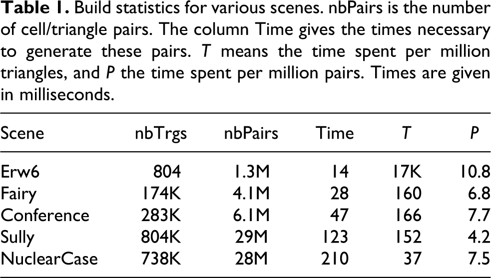
Table 1 clearly shows that the construction time does not depend on the number of triangles of the scene, but on the number of triangle/cell pairs that can be found in the triangle-oriented grid. This observation is based on the values of the coefficients P and T giving the number of milliseconds necessary to treat one million triangle/cell pairs and one million triangles, respectively. In contrast to T, the value P seems quite stable in the different scenes. This observation confirms the fact that our algorithm is not limited by the number of triangles in the scene, but by their respective width.

6.3 Exhaustive intersection computation

Performances of our overall algorithm are reported in Table 2 . The rays thrown are 1,024 × 1,024 primary rays. In such a case, some optimizations such as those done in rasterization could have been investigated. However we did not want to modify our algorithm, in order to see how it could work without knowing that the rays are so regularly spaced. The ray construction time is not included in these results, which means that about 20 ms have to be added to compInter to obtain the overall time of the simulation in each case. This table clearly shows that most of the computation time is spent in the execution of the algorithm described in the Section 5. It should also be noted that the execution of the program for the NuclearCase scene required two loops of triangles in order to avoid memory overflow.

Table 2.

Intersection test statistics for 1,024 × 1,024 primary rays on various scenes. trgTrace stands for the time spent to execute the complete triangle-tracing algorithm presented in Section 5, and compInter is the overall time of the simulation (except for the ray grid construction time). Times are given in milliseconds.

Scene	nbTests	nbInters	trgTrace	compInter
Erw6	1.3M	1.2M	48.3	56.9
Fairy	4.0M	1.8M	73.3	84.1
Conference	6.1M	2.7M	125.9	143.5
Sully	29.1M	3.7M	305	325.4
NuclearCase	14.0M	10.3M	498.4	517.9

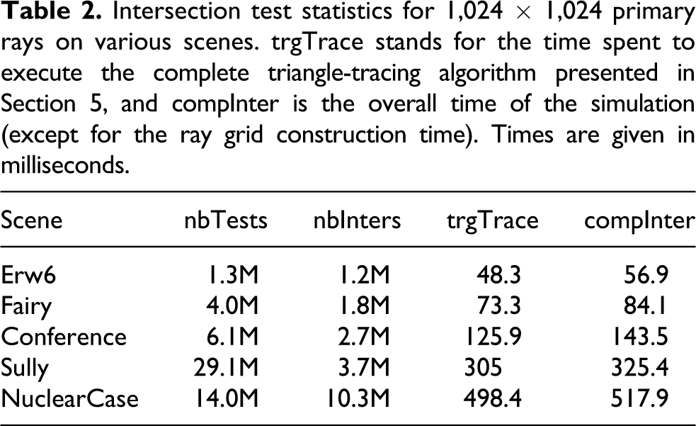
Figure 5 shows more precisely how the time is used during the execution of this phase. It should be noted that the intersection requests are not the bottleneck of these computations. The major step of the algorithm is the generation of the triangle/cell pairs (rasterization step), but all of the steps contribute to the computation time in a noticeable way. The rasterization step could certainly be improved by using more adapted rasterization techniques, such as that of Eisenacher and Loop (2010), but this would not modify our results by an order of magnitude. For most of the scenes, we are able to achieve 20 million intersections per second, which is quite good, since all of these intersections are sorted, and since the generation of all of the intersections produces a lot of overhead to prepare the memory for writing the results.

Figure 5.

Times for the different stages of the algorithm described in Section 5 (in milliseconds). The last step of the algorithm (sorting the coordinates for each ray) is not included.

To compare these results, we also implemented the classical algorithm, i.e. we generated the triangle grid and then scanned the different rays of the scene. Since these algorithms share lots of common operations, it is very simple to compare them. On the one hand, the classical algorithm builds the triangle grid and generates the list of ray/cell pairs. On the other hand, the triangle-tracing algorithm builds the ray grid and generates the list of ray/triangle pairs. It also has to sort the intersections by the index of the ray at the end of the computations. Since the time to generate the list of ray/cell pairs for the classical algorithm is not relevant (about 1 ms for one million rays), we just have to compare the triangle grid construction time with the sum of the three steps only executed in our algorithm. The results are given in Table 3 . First, it should be noted that the triangle grid could not be generated on the NuclearCase, because the amount of memory available on the GPU was not enough to generate the grid (985 MB of memory would have been necessary for this case). It reminds us that one of the reasons for inverting the classical algorithm was that it would solve these kinds of memory overflow issues. Then, it can be seen that the classical algorithm is clearly less efficient than the ray grid, especially when the size of the scene increases.

Table 3.

Comparison between the triangle tracing and the classical algorithm. pairsConstr is the time used to build the cell/triangle pairs for the triangle-tracing algorithm, and sortInters the time needed to sort the intersections by the index of the ray. Total results from the sum of these two numbers added to the ray grid construction time. It has to be compared with trgGrid, giving the construction time of the classical triangle grid. Times are given in milliseconds.

Scene	pairsConstr	sortInters	Total	trgGrid
Erw6	14.0	10.8	44.8	33.2
Fairy	28.3	15.0	63.3	69.2
Conference	46.6	21.7	88.3	108.0
Sully	123.4	30	173.4	408.9
NuclearCase	210.0	108.0	318.0	X

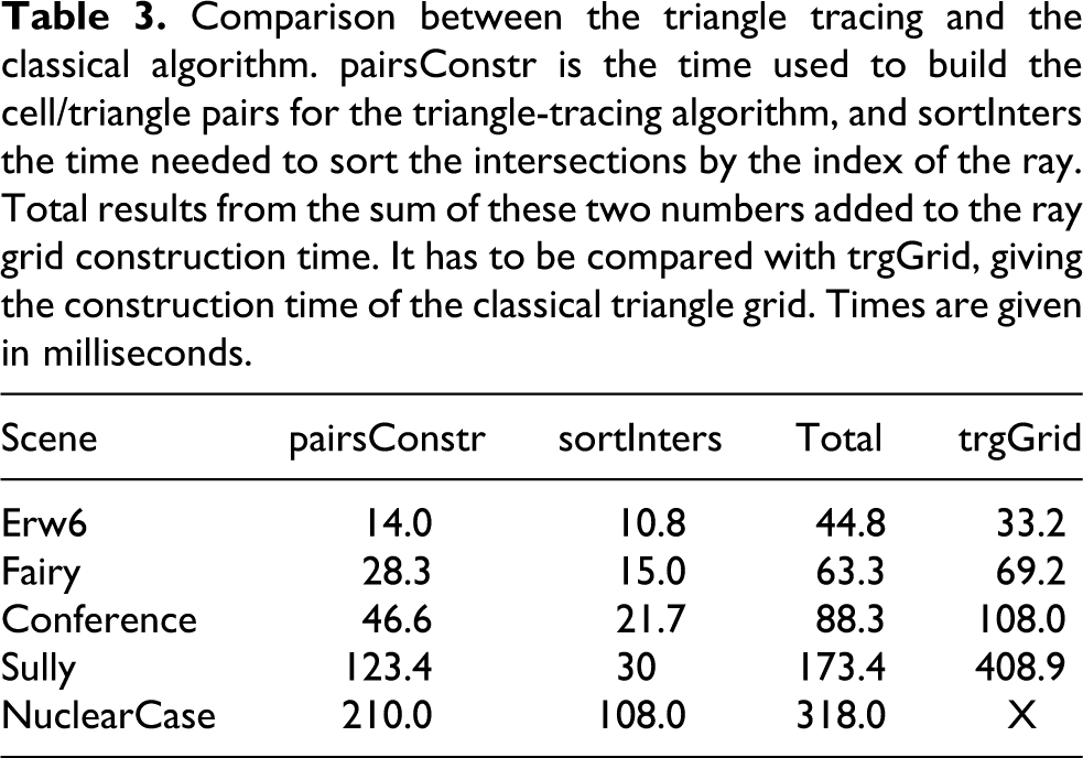
This can easily be explained: as seen above, the bottlenecks of the grid constructions are the sorts that have to be done on the ray/cell pairs (for the ray grid) and triangle/cell pairs (for the triangle grid). The number of triangle/cell pairs will for most cases be far greater than the number of ray/cell pairs (at most equal to the number of rays). This can lead to a very longer sorting time for the triangle grid, as can be seen on the Sully case. The drawback of our method is that we have to sort the intersections by the index of the ray, whereas they are already sorted in the classical algorithm. However, for most cases (especially large scenes), it is not enough to compensate for the time lost in sorting the triangle/cell pairs in the classical algorithm.

Our method allows us to correctly manage scenes composed of a high number of triangles. However, the problem is still open in the case of a scene generating a very high number of intersections: if in a given time the number of intersections is important (several dozen millions of intersections), the storage of these intersections, combined with the memory needs of the triangle-tracing algorithm, is a limiting factor. One solution to this problem would be to transfer the intersections to the CPU as soon as they are identified, while the calculation continues on the GPU for a new group of triangles, using asynchronous memory transfers, made possible with recent GPUs. However, this would impact the sorting of the intersections along each ray, since between different groups of triangles, new intersections can be found with rays already intersected by previously treated triangles. We would then have to efficiently handle the merge of the different groups of intersections on the CPU. Even though this problem only appears for a very high number of intersections, thus for scenes with a specific configuration, it would be worth treating it in the future.

We decided not to implement a BVH or other classical acceleration structures, because the perspective grid is clearly the structure that implies the fastest traversal time. This allows a fast access to the potentially intersecting rays for each triangle, once the cells it overlaps have been found. With a classical structure such as a BVH, the traversal time for one ray can be very long: in order to compute all intersections for each ray, we would first need to determine for each ray how many intersection tests have to be performed, then again performing this traversal to write the associated indices of triangles in memory, and finally run the tests. This would easily lead to load-balancing issues that are avoided here. Moreover, the construction times of the BVHs are clearly too elevated in the case of dynamic scenes, especially compared with our grids.

6.4 Experimentations on a nuclear-like scene

Finally, we tried to execute a test case representative of the usages envisaged for the nuclear industry. We defined six groups of 100,000 points, representing the sources of radiation of the NuclearCase scene. All rays thrown in our test case start from the same point (representing the point where the dose has to be measured), and end at one of the points described in our separate file.

These rays and the overall scene are seen through an external camera. When a ray passes through the air, it is colored in white, and it becomes red when passing through an object (see Figure 1). To detect whether a ray enters into an object or leaves it, we consider that the starting point of the rays is not included in any object of the scene. Thus, since the scene is very clean, the first intersection found along a ray can be considered as an entry point in an object, and the next will be the exit point of this object.

We were able to compute and sort about 6 million intersections in each step of the simulation, in a time of 400 ms. The difficulty here was that six grids had to be generated to cover the whole space. To be more efficient, and avoid storing memory for cells that will, certainly, not generate any intersection, we used the bounding boxes of the groups of sources. The first step in the computation consisted of testing whether the triangles were overlapped by these boxes, and to discard them if not. We also tried to use the fact that the NVIDIA GTX 295 is in fact the union of two GPUs. Thus, we used another card to display the graphics, and we tried to distribute the computations over the two GPUs. We tried two different strategies: the first only consisted in giving three grids to the first GPU, and the three others to the second. The second strategy consisted in arbitrarily splitting the triangles into two groups of same dimension and to make each GPU work on a different group (here, each GPU still had to handle six grids to cover the whole space). The first was the most efficient here: we could achieve a total time of 250 ms for the overall simulation, while we only achieved a time of 350 ms with the second strategy.

This can be explained by the good repartition of the six groups of rays over the scene in this case. However, it is clearly a problem that needs to be investigated in the future.

7 Conclusion

We have proposed a new GPU algorithm designed to compute every intersection between highly coherent rays and a complex 3D scene. In order to increase performance and avoid memory overflow issues, we introduced the use of a ray grid in perspective space. We postpone the partial building of the triangle grid after the building of the triangle grid. All of the algorithms proposed are designed to efficiently manage the finding of all of the intersections along each ray, which can sometimes lead to solutions fundamentally different from those used in traditional ray tracing.

This algorithm can also be very useful in a multi-GPU application, since each GPU can process the computations for a different bunch of triangles. As seen above, a simple repartition of the different triangles between the different GPUs is not very efficient. Strategies for efficiently distributing the triangles over the GPUs could bring much higher performance, and should be investigated in the future. Another extension of this work is the management of scenes generating a very high number of intersections, since the memory needed to store these intersections can also become a limiting factor for these scenes.

Footnotes

Funding

This research received no specific grant from any funding agency in the public, commercial, or not-for-profit sectors.

References

Aila

Laine

(2004) Alias-free shadow maps. In Proceedings of Eurographics Symposium on Rendering 2004.Aire-la-Ville, Switzerland: Eurographics Association, pp. 161–166.

Assad

Chiron

Nimal

J-C

Diop

Ridoux

(1999) General formalism for calculating gamma-ray buildup factors in multilayer shields into MERCURE-6 code. In Proceedings of the Ninth International Conference on Radiation Shielding. Tokyo: Atomic Energy Society of Japan, p. 493.

Bavoil

Callahan

Lefohn

Comba

JLD

Silva

(2007) Multi-fragment effects on the GPU using the k-buffer. In I3D’07: Proceedings of the 2007 Symposium on Interactive 3D Graphics and Games. New York: ACM Press, pp. 97–104.

Billeter

Olsson

Assarsson

(2009) Efficient stream compaction on wide SIMD many-core architectures. In HPG’09: Proceedings of the Conference on High Performance Graphics 2009. New York: ACM Press, pp. 159–166.

Cadet

Lecussan

(2007) Coupled use of BSP and BVH trees in order to exploit ray bundle performance. In RT’07: Proceedings of the 2007 IEEE Symposium on Interactive Ray Tracing. Washington, DC: IEEE Computer Society, pp. 63–71. ISBN 978-1-4244-1629-5.

Carpenter

(1984) The A-buffer, an antialiased hidden surface method. SIGGRAPH Comput Graph 18: 103–108.

Carr

Hall

Hart

(2002) The ray engine. In HWWS’02: Proceedings of the ACM SIGGRAPH/EUROGRAPHICS conference on Graphics hardware. Aire-la-Ville, Switzerland: Eurographics Association, pp. 37–46.

Catmull

(1974) A Subdivision Algorithm for Computer Display of Curved Surfaces. PhD thesis University of Utah (Department of Computer Science), USA.

Eisenacher

Loop

(2010) Data-parallel micropolygon rasterization. In Seipel

Lensch

(eds). Geneve, Switzerland: Eurographics 2010 Annex: Short Papers.

10.

Everitt

(2001) Interactive Order-Independent Transparency. Technical report, NVIDIA.

11.

Hoberock

Bell

(2009) Thrust: A Parallel Template Library, Version 1.2. http://www.meganewtons.com/.

12.

Houston

Preetham

Segal

(2005) A hardware F-buffer implementation. In Meissner

Schneider

B-O

(eds).

13.

Hunt

Mark

(2008) Ray-specialized acceleration structures for ray tracing. In IEEE/EG Symposium on Interactive Ray Tracing 2008. IEEE/EG, pp. 3–10.

14.

Ivson

Duarte

Celes

(2009) GPU-Accelerated Uniform Grid Construction for Ray Tracing Dynamic Scenes. Technical Report 14/09, Pontifícia Universidade Católica do Rio de Janeiro, Departamento de Informática.

15.

Ize

Wald

Parker

(2007) Asynchronous BVH construction for ray tracing dynamic scenes on parallel multi-core architectures. In Proceedings of the 2007 Eurographics Symposium on Parallel Graphics and Visualization.

16.

Johnson

Lee

Burns

Mark

(2005) The irregular Z-buffer: hardware acceleration for irregular data structures. ACM Trans Graph 24: 1462–1482.

17.

Jouppi

Chang

(1999) Z3: an economical hardware technique for high-quality antialiasing and transparency. In HWWS’99: Proceedings of the ACM SIGGRAPH/EUROGRAPHICS workshop on Graphics hardware. New York: ACM Press, pp. 85–93.

18.

Kalojanov

Slusallek

(2009) A parallel algorithm for construction of uniform grids. In HPG’09: Proceedings of the Conference on High Performance Graphics 2009. New York: ACM Press, pp. 23–28.

19.

Lagae

Dutré

(2008) Compact, fast and robust grids for ray tracing. Computer Graphics Forum 27: 1235–1244.

20.

Lauterbach

Garland

Sengupta

Luebke

Manocha

(2009) Fast BVH construction on GPUs. Computer Graphics Forum 28: 375–384.

21.

Lauterbach

Yoon

S-E

Manocha

(2006) RT-DEFORM: interactive ray tracing of dynamic scenes using BVHs. In Proceedings of the 2006 IEEE Symposium on Interactive Ray Tracing, pp. 39–45.

22.

Liu

Huang

M-C

Liu

X-H

E-H

(2009) Efficient depth peeling via bucket sort. In HPG’09: Proceedings of the Conference on High Performance Graphics 2009. New York: ACM Press, pp. 51–57.

23.

Mark

Proudfoot

(2001) The F-buffer: a rasterization-order FIFO buffer for multi-pass rendering. In HWWS’01: Proceedings of the ACM SIGGRAPH/EUROGRAPHICS workshop on Graphics hardware. New York: ACM Press, pp. 57–64.

24.

Merrill

Grimshaw

(2010) Revisiting sorting for GPGPU stream architectures. In Proceedings of the 19th international conference on Parallel Architectures and Compilation Techniques (PACT’10). New York: ACM Press, pp. 545–546.

25.

NVIDIA (2009) Cuda Zone, The resource for CUDA Developers. http://www.nvidia.com/object/cuda_home.html.

26.

OpenCL (2009) http://www.khronos.org/opencl/.

27.

Reshetov

Soupikov

Hurley

(2005) Multi-level ray tracing algorithm. In SIGGRAPH’05: ACM SIGGRAPH 2005 Papers. New York: ACM Press, pp. 1176–1185.

28.

Satish

Harris

Garland

(2009) Designing efficient sorting algorithms for manycore GPUs. In IPDPS’09: Proceedings of the 2009 IEEE International Symposium on Parallel and Distributed Processing. Washington, DC: IEEE Computer Society, pp. 1–10.

29.

Sengupta

Harris

Zhang

Owens

(2007) Scan primitives for GPU computing. In GH’07: Proceedings of the 22nd ACM SIGGRAPH/EUROGRAPHICS symposium on Graphics hardware, Vol. 3. Aire-la-Ville, Switzerland: Eurographics Association, pp. 97–106.

30.

Wald

(2004) Realtime Ray Tracing and Interactive Global Illumination. PhD thesis, Computer Graphics Group, Saarland University.

31.

Wald

Boulos

Shirley

(2007) Ray tracing deformable scenes using dynamic bounding volume hierarchies. ACM Trans Graph 26: 6.

32.

Wittenbrink

(2001) R-buffer: a pointerless A-buffer hardware architecture. In HWWS’01: Proceedings of the ACM SIGGRAPH/EUROGRAPHICS Workshop on Graphics Hardware. New York: ACM Press, pp. 73–80.

33.

Zhou

Hou

Wang

Guo

(2008) Real-time KD-tree construction on graphics hardware. ACM Trans Graph 27: 1–11.