
Abstract
The Community Climate System Model (CCSM) has been developed over the last decade, and it is used to understand past, present, and future climates. The latest versions of the model, CCSM4 and CESM1, contain totally new coupling capabilities in the CPL7 coupler that permit additional flexibility and extensibility to address the challenges involved in earth system modeling. The CPL7 coupling architecture takes a completely new approach with respect to the high-level design of the system. CCSM4 now contains a top-level driver that calls model component initialize, run, and finalize methods through specified interfaces. The top-level driver allows the model components to be placed on relatively arbitrary hardware processor layouts and run sequentially, concurrently, or mixed. Improvements have been made to the memory and performance scaling of the coupler to support much higher resolution configurations. CCSM4 scales better to higher processor counts, and has the ability to handle global resolutions up to one-tenth of a degree.
Introduction
Background
Climate modeling is a complex multi-physics application and is one of today’s high-performance computing challenges. The Community Climate System Model (CCSM) is a coupled, state-of-the-art global climate model consisting of four fundamental physical components: an atmosphere model, a surface land model, an ocean model, and a sea-ice model. The Community Earth System Model (CESM) adds a new land ice component, land and ocean biogeochemistry functionality, an atmospheric chemistry model, and a capability for the atmospheric component to span a larger range of altitudes. The CCSM and CESM components can be either ‘data’ components, which read coupling data from files, or ‘active’ dynamical components, which predict coupling fields prognostically. Each dynamical component typically contains both fluid-dynamics solvers and detailed parameterizations to compute the internal and external forcing terms that arise from such diverse phenomena as the passage of radiation through the atmosphere, the release of latent heat by phase changes of water, and the effects of friction and unresolved turbulent scales.
As the CCSM/CESM components compute forward in time, they periodically exchange boundary data via the use of coupling software. This coupling software supports communication of data between components, interpolation of data between different component grids, merging of fields from several ‘source’ components to a ‘destination’ component, and the production of various diagnostics, such as global surface heat flux budgets, among other things. CCSM3 (Collins et al., 2006a) used the CPL6 coupling software (Craig et al., 2005). In what follows, we present an overview of the high-level design and performance of the new CPL7 coupling software that forms an integral part of CCSM4 and CESM1. In the following discussion, the names ‘CCSM4’ or ‘CPL7’ will be used to describe capabilities in both CCSM4 and CESM1.
Couplers are a key component of climate models. In particular, coupling of models normally involves at least three different aspects: the coupling architecture, the communication infrastructure, and the coupling methods. The coupling architecture is generally associated with the overall control of the system, including the temporal sequencing of the model components. The communication infrastructure supports data transfer between components and, depending on the overall design, can be implemented from a high-level driver through subroutine calls or from within the model components directly. Finally, coupling methods provide capabilities, such as mapping (interpolation), between different component grids, merging from several source components to a destination component, computation of physical quantities such as fluxes, or the computation of diagnostics. Every coupled climate model application needs to address these aspects, and they are generally implemented using a combination of community tools (such as ESMF, MCT, PRISM, MPI, or NETCDF) and custom-built software.
Coupling architectures can be broadly categorized by four basic features: whether data is sent through a specific coupler ‘hub’ or communicated directly between components, whether communication of data is handled via a top-level driver or from calls directly within the components, whether the coupled model components are run on overlapping or distinct hardware processors, and whether a system is run as a single executable or as multiple executables. The CCSM has always had, and continues to have, a hub design. Over the last five years, however, the CCSM has migrated from a multiple executable, fully concurrent, direct coupling architecture to a single executable architecture with flexible component layout on processors and a top-level driver. To couple models developed separately into a single application, the CCSM has always made efforts to design coupling architectures that permitted coupling with minimum modification to component models regardless of the approach.
When discussing coupled applications, it is important to distinguish between temporal concurrency and processor concurrency. Temporal concurrency is a capability within a scientific application to execute parallel in time. It is the ability to run work in parallel on multiple processors without dependencies that impose strict sequencing. Processor concurrency is the act of giving different pieces of work unique hardware processors, typically through spatial domain decomposition. Two models will run concurrently across processors only if they are run on unique sets of processors and if there are no temporal dependencies between the components that will limit concurrency.
Single executable designs do not automatically imply that models are running on the same processors sequentially. In general, components can be laid out in relatively arbitrary processor groups with single executable systems. On the other hand, multiple executable systems normally imply that the model components are running concurrently on unique processors, since operating systems (OSs) and queuing software generally disallow multiple executables from sharing the same hardware processors and interleaving.
A particular coupled climate model implementation is fundamentally driven by architectural choices related to component sequencing, coupling frequency and lags, concurrency, scientific requirements, job launching, component integration, and interoperability. Climate models developed over recent decades exhibit different architecture choices. For example, the Parallel Climate Model (PCM; Washington et al., 2000) incorporated a high-level driver that supported sequential execution of components in a single executable. In this case, the coupler was a driver that called components via subroutine interfaces and the sequencing and coupling operations were custom built around particular scientific needs. On the other hand, the OASIS coupler (Valcke et al., 2006) is a more generic coupler component designed to support coupling of multiple executable components that communicate via calls to a shared coupling interface called PSMILe (Redler et al., 2010). OASIS supports both coupling through a hub and direct coupling between components. The design of these two couplers is fundamentally different, yet they both meet the scientific needs of their community. Other examples of climate model couplers are FMS (http://www.gfdl.noaa.gov/fms), the custom coupler in FOAM (Jacob et al., 2001), PALM (http://www.cerfacs.fr/globc/PALM_WEB) and FLUME (http://research.metoffice.gov.uk/research/interproj/flume/). Other examples of coupling libraries are MCT (Larson et al., 2005), ESMF (Hill et al., 2004), and the Distributed Data Broker (Drummond et al., 2001).
Motivation
Prior to CCSM4, the CCSM operated as a multiple executable system where all models ran concurrently over disjoint sets of hardware processors and where each component model was a separate binary program. The components started independently and communicated to the coupler at regular intervals via send and receive methods placed directly within each component. The coupler was a separate binary and acted as a central hub coordinating data exchange, managing lags and sequencing, and executing coupler operations such as mapping (interpolation) and merging. In practice the model timestepping was difficult to understand because of a lack of transparency between the coupler sequencing and the embedded communication calls in components. In addition, although special efforts were made in CCSM3 to maximize the amount of concurrency to increase throughput, the multiple executable concurrent design limited model throughput in some configurations. The CCSM3 design also made porting and debugging challenging on occasion, largely because of the lack of support for multiple executable job launches on some platforms. Finally, the prior CCSM implementations were not consistent with an ability to couple using standards promoted by the Earth System Model Framework (ESMF).
Recent advances in physics algorithms in CCSM4 components, including an updated and improved atmospheric boundary layer scheme and new radiation and surface albedo algorithms, require that components be coupled more frequently than in the past for stability reasons. In addition, as resolutions increase, component timesteps decrease and coupling frequencies tend to increase. With the recent need for higher frequency coupling, limitations in the CCSM3 capability to overlap work in concurrent execution became increasingly critical.
In the past, the atmospheric component of the CCSM, CAM (Collins et al., 2006b), and the land component, CLM (Bonan et al., 2002; Oleson et al., 2010), have been made available as distinct ‘stand-alone’ coupled systems with all components running on the same grid. They are extensions of the prior CCM and LSM release models that have existed at the National Center for Atmospheric Research (NCAR) since the 1980s. The CAM ‘stand-alone’ model was an atmosphere, land-surface, data-ocean (using prescribed sea surface temperatures), and thermodynamic-only sea-ice (using prescribed ice coverage) coupled system. The CLM ‘stand-alone’ model consisted of data-atmosphere and prognostic land-surface coupled components. Over the past decade, these ‘stand-alone’ models were released and supported in parallel to the CCSM. CCSM4 wanted to duplicate several features associated with the CAM and CLM ‘stand-alone’ systems, such as an ability to run sequentially on a single processor to support the current CAM and CLM ‘stand-alone’ communities without a distinct ‘stand-alone’ release. The new CCSM4 coupler was designed to allow this.
The effort to update the CCSM coupling architecture was undertaken for several reasons, including an ability to better support new science, a desire to support fully sequential and single processor integration, the migration to a single executable system for ease in porting and use, an increased flexibility of component layouts on hardware processors to improve performance over a wider range of problems, an ability to support coupling via the ESMF specification, and the capability to run much higher resolutions and higher processor counts with improved performance and memory scalability.
Design
Overview
With CPL7 in CCSM4, a completely new approach has been taken with respect to the high-level architecture and design of the system. The system is now controlled by a top-level driver that runs on all processors, and components are run via calls to standard subroutine interfaces that run on all or arbitrary subsets of hardware processors. The driver also calls coupler methods to map (interpolate) fields, rearrange data, merge fields, calculate fluxes, and generate diagnostics. In CCSM4, the coupler methods run on a distinct subset of all the processors as if the coupler were a separate component. In effect, the CPL6 sequencing and hub attributes have been migrated into a driver, while the CPL6 coupler operations are carried out on a subset of the processors within the driver as if there is a separate coupler component.
CCSM4 has greatly expanded the flexibility of component layouts by moving to a single executable system that continues to support concurrent processor layouts but also supports components running sequentially or in mixed sequential/concurrent mode. This new wider layout choice gives users more flexibility in optimizing load balance and efficiency for any simulation configuration. CPL7 was also rewritten to significantly reduce memory use and improve memory scaling. Previous CCSM versions were run mostly at global resolutions of one to five degrees, and memory usage was not a constraint. CCSM4 now supports the ability to run global one-tenth degree resolutions using tens of thousands of processors on massively parallel machines with relatively limited memory available per processor, especially given the problem size.
CCSM4 supports both data and active component models. In CCSM4, like CCSM3, the atmosphere, land, and sea-ice models are always ‘tightly’ coupled (Larson, 2009) to better resolve the diurnal cycle. This coupling is typically half-hourly, although is often more frequent at higher resolutions. It is important to point out that while atmosphere/land and atmosphere/ice fluxes are computed in the land and ice component models, respectively, atmosphere/ocean fluxes are computed in the coupler (and not in the ocean component) at the same frequency that the atmosphere, land, and sea-ice models communicate. Similarly, the diurnal cycle of ocean surface albedo is also computed in the coupler for use by the atmosphere model. Since the ocean model is not responsible for computing atmosphere/ocean fluxes, it is typically coupled once or a few times per day. The looser ocean coupling frequency means the ocean state and response is lagged in the system. This also permits the ocean model to run on a mutually exclusive set of processors from the atmosphere, land, sea-ice, and coupler components. There is an option in CCSM4 to run the ocean tightly coupled with reduced lags, but this is normally used only when running with a data-ocean component.
Depending on the resolution, hardware, run length, and physics, a CCSM4 run can take several hours to several months of wall clock time to complete. Runs typically encompass model simulation times of decades or centuries, with the model typically running between one and fifty simulated years per wall clock day. CCSM4 has an ‘exact restart’ capability, which allows the model to be stopped and restarted as if it had never stopped, and the model is typically run in one year or multi-year periods per invocation to fit within wall clock limits at production computing facilities.
Sequencing and concurrency
CCSM4 uses the Message Passing Interface (MPI) for all inter-model and most intra-model communication. Many components can use a hybrid mode of parallelism using OpenMP threads within each MPI task. In CCSM4, the component processor layouts and MPI communicators are derived from simple user-specified namelist input. Presently, there are seven basic MPI processor groups in CCSM4. These are associated with the atmosphere, land, ocean, sea-ice, land-ice, coupler, and ‘world’ groups, although others can be added easily. The driver runs on all processors using the ‘world’ group, while the coupler group, which carries out coupler operations such as mapping and merging, is generally run on a subset of all processors. Each of the basic MPI groups can be associated with unique processors sets, and a user can overlap MPI groups on hardware processors relatively arbitrarily. If any processor groups overlap each other in at least one processor, then components in those groups will run sequentially. Each processor group is described at runtime using three scalar variables: the number of MPI tasks, the number of OpenMP threads per MPI task, and the global MPI task rank of the root process for that group. For example, a layout where the number of MPI tasks is 8, the number of threads per MPI task is 4, and the root process is MPI task 16 would create a processor group that consisted of 32 hardware processors, starting at global MPI task number 16, and it would contain 8 MPI tasks. The CPL7 driver derives all MPI communicators at initialization and passes them to the component models for use. This input information is used both to set MPI groups and to set batch- and job-launching parameters.
As mentioned in the introduction, there are two aspects that determine whether component models run concurrently. The first is whether unique chunks of work are running on distinct processor groups. The second is the sequencing of this work in the driver. As much as possible, the CCSM4 driver sequencing has been implemented to maximize the potential amount of concurrency between components. Ideally, in a single coupling step, the forcing for all models would be computed first. The models could then all run concurrently, and then the driver time would advance. However, scientific requirements, such as the coordination of surface albedo and atmospheric radiation, as well as boundary layer stability, impose constraints on the coupling lags. Figure 1 shows the maximum amount of concurrency currently supported in the CCSM4 driver for a fully active system configuration. More concurrency is technically possible, but the scientific constraints impose a limitation on the coupling between the atmosphere model and the land and sea-ice models such that the atmosphere model runs sequentially with both of those surface models. Figure 1 does not necessarily represent the optimum processor layout for performance for any configuration, but provides a practical limit to the amount of concurrency currently supported in the system. It is important to point out that, with CCSM4, results are identical to numerical round-off regardless of the layout of components on processors. Results are not bit-for-bit identical in this case, because some physical components introduce round-off level changes when changing processor counts.
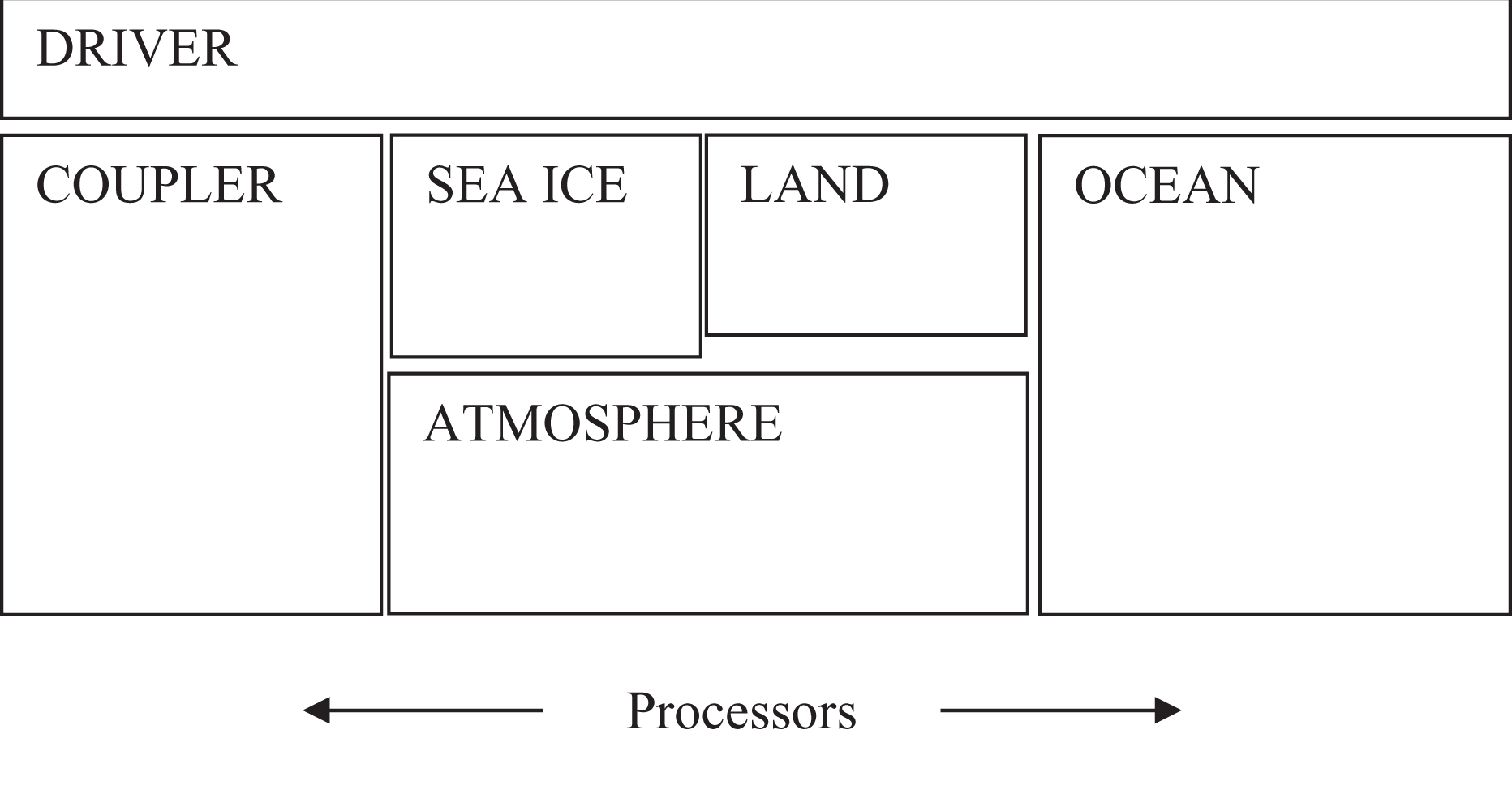
CCSM4 concurrency capability based on scientific constraints.
There is a loss of concurrency in CCSM4 relative to CCSM3. In CCSM4, the model run methods are called from the driver, and the coupling from the overall system perspective looks like ‘send to component, run component, receive from component’. In CCSM3, the coupling was done via direct calls from inside each component and the send and receive calls could be interleaved with work such that the model run method appeared to have two phases: one between the coupling send and receive, the other between the receive and send. Although that allowed greater concurrency in CCSM3, it was also designed for concurrent-only execution. In CCSM4, multiple run phases were not implemented in order to simplify the model coupling interfaces to support data and active versions of components more easily. This choice was made with the full understanding that there would be some potential loss of model concurrency in specific cases. However, it was felt that the additional flexibility of allowing models to run in a mixed sequential/concurrent system would overcome any performance degradation due to a potential loss of concurrency.
The CCSM4 component model interfaces consist of initialize, run, and finalize methods with consistent arguments across different component models. Although the standard CCSM4 component interface arguments currently consist of Fortran and Model Coupling Toolkit (MCT; Jacob et al., 2005; Larson et al., 2005) datatypes, alternative component interfaces are available for each model component that are consistent with the ESMF gridded component specification. In this case, ESMF interfaces are implemented as a wrapper layer in the CCSM components without any fundamental changes to the coupler or physical components.
The driver/coupler acquires all information about resolution, configurations, and processor layout at runtime from either input files or from communication with components. Initialization of the system in CCSM4 is relatively straightforward. First, the varied MPI communicators are set up in the driver. Then the component initialization methods are called on the appropriate processor groups, and grid and decomposition information is passed back to the driver. Once the driver has the grid and decomposition information from the components, various datatypes are initialized that will move data between processors, decompositions, and grids as needed at the driver level. The coupling implementation does not treat components running on identical or distinct processors differently. However, in cases where the grid, decomposition, and processor layout are identical between two components, the data movement will degenerate to a local data copy, avoiding the communication network hardware and most of the communication software stack. The physical coupling fields are passed through the interfaces in the initialize, run, and finalize phases. The run interface also contains a clock data instance that specifies the current time and the run length for the model.
The sequencing of the driver run loop for the CCSM4 configuration with coupler, land, sea-ice, atmosphere, and ocean components is shown in Figure 2 . The order of operations is hard-wired in the CCSM4 driver and is based on scientific constraints first and performance optimization second. The boxes indicate work and the horizontal arrows represent coupling. The sizes of the boxes are not indicative of the relative time taken. The communication between the coupler and a component introduces a cross-component dependency, where one component will normally wait for the other component before communication proceeds. Coupling to the atmosphere, land, and sea-ice models occurs every step through the run loop, while coupling to the ocean normally occurs less frequently with additional temporal data lags. Figure 2 shows that if components are run concurrently, the ocean will begin first, followed by the land and sea ice. The atmosphere model will not start until data from the sea-ice and land models is communicated to the coupler. That data is needed to generate coupling data for the atmosphere model and is sent to the atmosphere component. The ocean is able to integrate concurrently with all other components in the design. Figure 2 provides the detailed implementation that limits the total amount of concurrency shown in Figure 1. It is important to stress that the layout of components on processors does not change the model sequencing or results. The coupler is constantly computing between communication steps, and some of this work is overlapped with other components. Generally, the coupler work and communication costs are small compared to the active model run times.
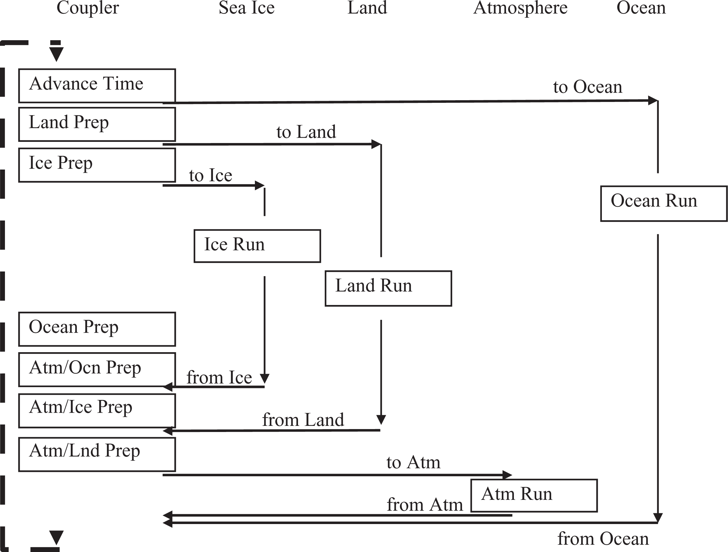
Driver loop sequencing showing the order of operations at the driver level. The boxes represent work and the horizontal arrows represent data coupling. The driver timestep loop is indicated by the dashed line.
CPL6 was built using the MCT infrastructure library, and CPL7 continues to rely heavily on MCT. MCT supports many critical coupling needs, such as managing data parallelism (the communication architecture of a coupler) and performing parallel mapping (one of the coupling methods). The high-level datatypes in CPL7 consist largely of MCT datatypes, and MCT is used for all data rearrangement and data mapping between component processors, decompositions, and grids. Although the CPL7 coupling architecture is dependent on MCT infrastructure, the high-level superstructure is designed to be compatible with ESMF (Collins et al., 2005), and CCSM4 components are ESMF-compliant. Mapping weights are still generated offline using the SCRIP package (Jones, 1998). In order to minimize the memory footprint, mapping weights are read into CCSM4 using a method that reads and distributes the weights in reasonably small chunks.
CCSM4 targets much higher resolution options than previous CCSM versions. Efforts have been made to reduce the memory footprint and improve memory scaling in all components, including the coupler, with the goal of being able to run the fully coupled system at one-tenth degree global resolution on tens of thousands of processors, with each processor having as little as 512 MB of memory. This target limits the number of non-distributed arrays that can be allocated on any single processor to just a few at any time and has led to some significant component refactoring, especially in initialization. In addition, the memory required to carry out traditional serial input/output (I/O) at higher resolutions is unacceptable, and serial I/O performance at higher resolutions can be a significant performance bottleneck. To address I/O performance and memory usage in the model, PIO, a new parallel I/O library (Dennis et al., 2011b) was developed within the CCSM community providing uniform and flexible interfaces to NetCDF, pNetCDF (www.mcs.anl.gov/parallel-netcdf), and MPI-IO. All model components are currently using the PIO software extensively, and use of PIO along with model component refactoring permits CCSM4 to run at resolutions that were not previously possible.
Performance, scaling, and load balance
To target scaling to tens of thousands of processors, developers for all components have worked at improving performance scaling via changes to algorithms, infrastructure, and decompositions. In particular, decompositions using shared memory blocks, space filling curves (Dennis et al., 2011a), and all three spatial dimensions have been implemented to varying degrees in order to increase parallelization and improve scalability in all components, including the coupler.
CCSM4 load balancing involves determining the optimum component layout across processors in order to optimize performance and minimize idle time. CCSM4 performance, load balance, and scalability are constrained by the problem size, complexity, and multiple-model character of the system. Within the system, each component has its own scaling characteristics, and variation in scaling of a component occurs because of internal load imbalance, decomposition capabilities, or communication costs. Component performance can also vary as the model integrates forward in time. This occurs because of seasonal variability of the cost of physics in models, changes in performance during an adjustment (spin-up) phase, and temporal variability in calling certain model operations, such as radiation, dynamics, or I/O. Within these constraints, a load balance configuration with relatively small but non-zero idle time and reasonably good throughput is nearly always possible to configure with CCSM4. CCSM4 has significantly increased the flexibility of the possible processor layouts, and this has resulted in better load balance configurations compared to previous CCSM versions.
In practice, load-balancing CCSM4 involves a number of considerations, such as which components are run, the component resolutions, and the relative resolutions of different components; cost, scaling, and processor count capabilities for each component; and internal load imbalance within a component. It is often best to load balance the system with all significant runtime I/O turned off, because this generally occurs infrequently (typically one timestep per month in CCSM4), is best treated as a separate cost, and can bias interpretation of the overall model load balance. The ability to use OpenMP and the performance of OpenMP threading in some or all of the system is dependent on the hardware/OS support, as well as whether the system supports running all MPI and mixed MPI/OpenMP on overlapping processors for different components. Finally, the processor layout, whether sequential, concurrent, or some combination of the two, can be varied. Typically, a series of short test runs is done with the desired production configuration to establish a reasonable load balance setup for the production job. CCSM4 provides some post-run analysis of the performance and load balance of the system to assist users in improving the processor layouts.
Results
In this section, performance scaling results will be presented for four different coupler kernels. Then some full model results will be presented to show how the layout of components on hardware processors impacts overall model performance. The four kernels that will be discussed are a field merge on the ocean grid, an atmosphere-ocean flux calculation, a rearrangement of ocean data between two different decompositions, and an atmosphere to ocean mapping (interpolation). These kernels represent the most common CCSM coupler operations. Results will be presented for three different hardware platforms – bluefire, jaguarpf, and intrepid – and at two different model resolutions – a moderate ‘f19_g16’ resolution and a high ‘f05_t12’ resolution.
Bluefire is an IBM SP6 at the NCAR with 4096 4.7 GHz processors and 4 GB of memory per processor. Processors are grouped into 32-way nodes, and each processor supports up to 4 FLOPS (floating point operations) per clock cycle. The interconnect uses an InifiniBand switch, and each node has eight 4X DDR links. Bluefire supports simultaneous multi-threading (SMT), which allows 64 MPI tasks to be assigned to each node, and the SMT mode was used for all timing results on bluefire. Jaguarpf is a Cray XT5 at the National Center for Computational Sciences (NCCS) at Oak Ridge National Laboratory (ORNL) that has 18,688 nodes of dual hex-core AMD processors running at 2.6 Ghz with 16 GB of memory per node. The total number of processors available is 224,256, and the interconnect uses a SeaStar 2+ router. Intrepid is an IBM Bluegene/P at Argonne National Laboratory (ANL) with 163,840 850 MHz PowerPC 450 processors. There are 4 processors per shared memory node, 1024 nodes per rack, and each node has 2 GB of memory.
The moderate resolution grid, ‘f19_g16’, consists of a nominally two-degree atmosphere/land grid with 144 × 96 horizontal grid points coupled to a nominally one-degree ocean/ice grid with 320 × 384 grid points. The high-resolution, ‘f05_t12’, configuration has 576 × 384 grid points on a nominally half-degree atmosphere/land grid coupled to a nominally one-tenth degree global resolution ocean/ice configuration with 3600 × 2400 horizontal grid points. All cases were run with shared memory parallelism (OpenMP) turned off, and one MPI task was placed on each processor with the following exceptions: on bluefire, the IBM SP6, SMT mode was used as indicated above. On intrepid at the high-resolution ‘f05_t12’ configuration, one MPI task was assigned to each four-way node due to memory limitations.
Tests were carried out on all machines in a production environment. As a result, some variability in timings was observed. Cases were rerun as needed to try to understand the variability better and, generally, best times are shown. All cases were carried out as 20-day runs using a ‘dead’ model setup (which replaces physical components with analytical test data) without any history or restart I/O. All timers were isolated with MPI_BARRIER calls, and the time on the slowest task is presented. Over each 20-day integration, each kernel was called 960 times, and the time was summed over all calls and on each MPI task. The times presented in the plots are seconds per simulated model day. All results are plotted in log/log format, and each plot uses the same horizontal and vertical axis scales for easier comparison. In addition, the same linear scaling reference line is included in each plot, and the horizontal axis is the number of MPI tasks used by the coupler for the test case. Performance is based on standard ‘out-of-the-box’ CCSM compiler, batch, and environment settings for the CESM1 release without any additional case-by-case tuning.
Figure 3 shows performance of the ocean field merge kernel from the CCSM coupler. This kernel is responsible for merging various fields on the ocean grid from different components. This operation is trivially parallel (there is no communication), and the kernel is primarily memory access limited. At the higher ‘f05_t12’ resolution, the performance on all platforms is remarkably similar, with near-linear scaling to over 1000 processors on all machines. In contrast, the performance scaling of the moderate ‘f19_g16’ resolution case is near linear up to about 100 processors on all machines. Above about 100 processors, performance tails off on bluefire and intrepid, while jaguarpf performance tails off at about 1000 processors.
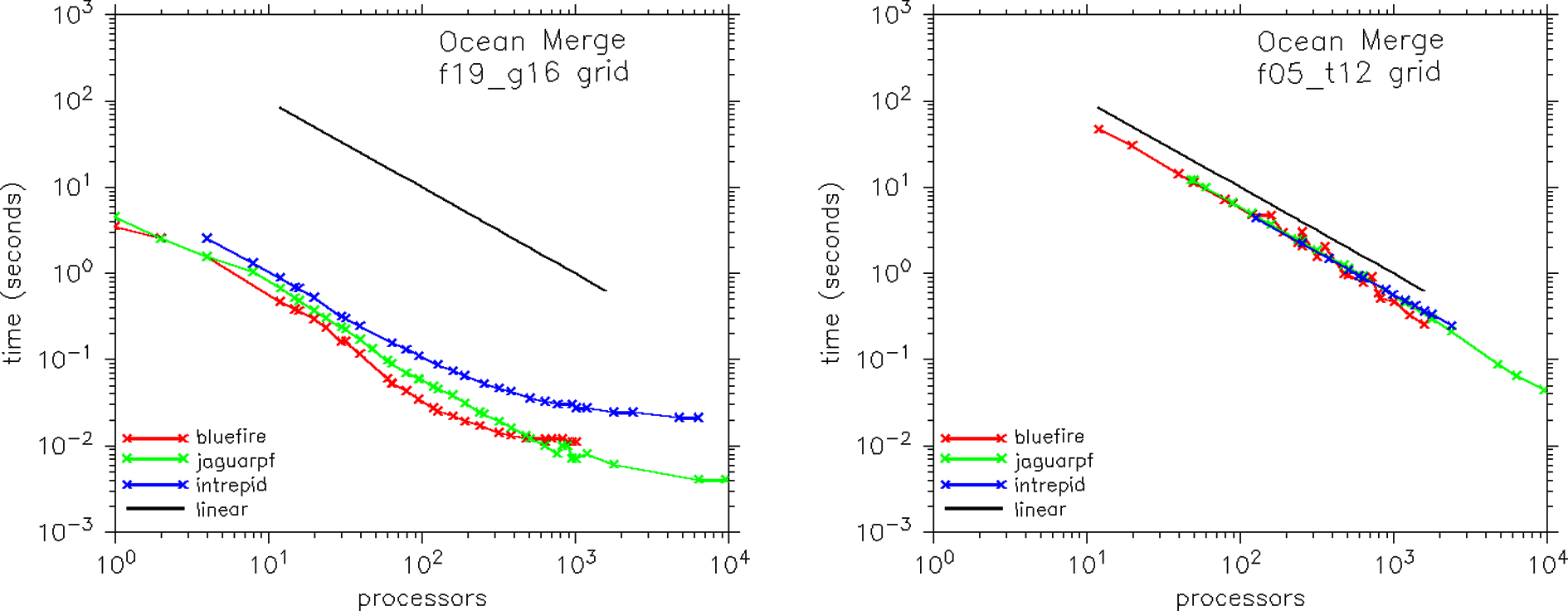
Scaling performance of the ocean merge kernel in the CCSM4 coupler at two resolutions (‘f19_g16’ and ‘f05_t12’) and on three hardware platforms (bluefire, jaguarpf, and intrepid).
Figure 4 shows the performance scaling of the atmosphere/ocean flux calculation. This calculation is also trivially parallel and is computed on the ocean grid. Compared to the ocean merge kernel, this computation is dominated by mathematical operations, including add, multiply, divide, min/max, log, exponential, and square root. The number of FLOPS per memory load in this kernel is relatively high and, compared to Figure 3, the scaling is near linear on all machines to at least 1000 processors, even at the moderate resolution. The absolute performance of this kernel on bluefire and jaguarpf is nearly identical, but intrepid, with 3–6 times slower processors, runs about 10 times slower than the other two machines on this highly FLOP-intensive metric.
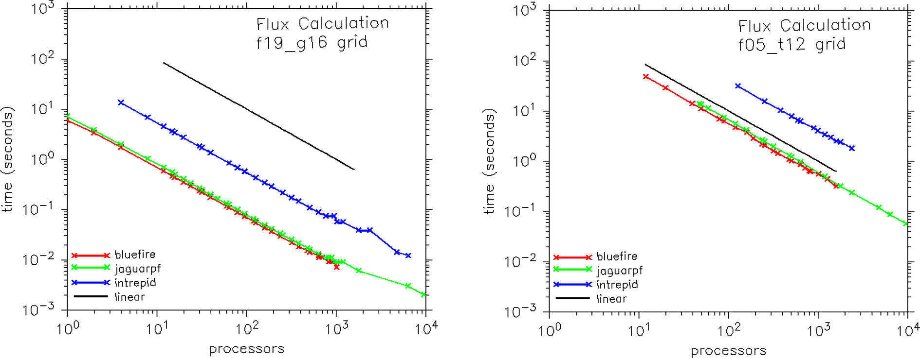
Scaling performance of the atmosphere/ocean flux kernel in the CCSM4 coupler at two resolutions (‘f19_g16’ and ‘f05_t12’) and on three hardware platforms (bluefire, jaguarpf, and intrepid).
Figure 5 documents the scaling performance of a rearrange operation on the ocean grid. There are no FLOPS in this kernel, just memory access and a MCT rearrange of data between an ocean decomposition and an ice decomposition of the same grid. This rearrange is nearly an all-to-all communication of data between processors, and is performance limited by the communication cost. Scaling is generally sublinear for both resolutions across the full range of test cases. The scaling tails off significantly above about 100 processors at the moderate ‘f19_g16’ resolution, with jaguarpf becoming slower (rolling over) above about 100 processors. At the higher ‘f05_t12’ resolution, scaling is somewhat better, but it still flattens out at about 500 processors on bluefire, flattens out at about 1000 processors on intrepid, and rolls over at about 500 processors on jaguarpf.
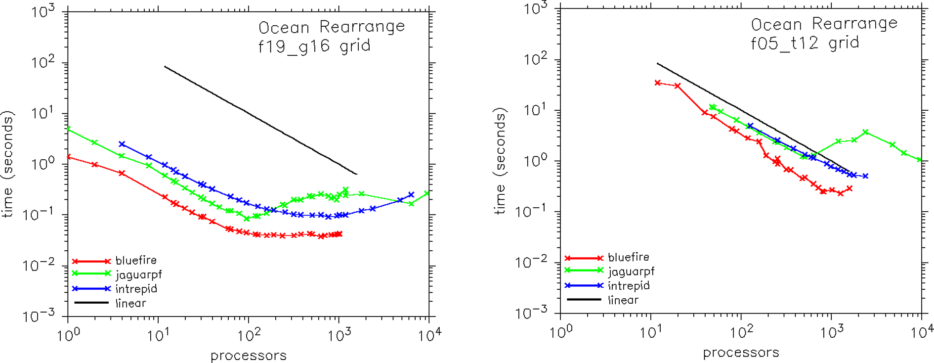
Scaling performance of the ocean to ice rearrange kernel in the CCSM4 coupler at two resolutions (‘f19_g16’ and ‘f05_t12’) and on three hardware platforms (bluefire, jaguarpf, and intrepid).
Figure 6 shows the atmosphere to ocean mapping (interpolation) performance in the CCSM. This kernel is a mixture of communication and multiply-add operations (Jacob et al., 2005) and is carried out using a MCT mapping method. In this case, the mapping weights are always distributed based on the ocean decomposition at initialization. When the kernel is called, the atmosphere data is rearranged to the ocean decomposition such that, for every processor, the atmosphere data required for mapping to the local ocean grid is available. For some atmospheric grid points, the data is rearranged to more than one ocean processor. When the rearrangement is complete, atmosphere data is locally interpolated to the ocean grid. Overall, the performance of this kernel is similar to the performance of the rearrange kernel in Figure 5, indicating the importance of the rearrange step in the overall cost of this operation. Scaling starts to go flat or even turns over at about 100 processors for all machines at the moderate ‘f19_g16’ resolution. The ‘f05_t12’ scales well to about 1000 processors, except on jaguarpf, where scaling flattens dramatically at about 500 processors.
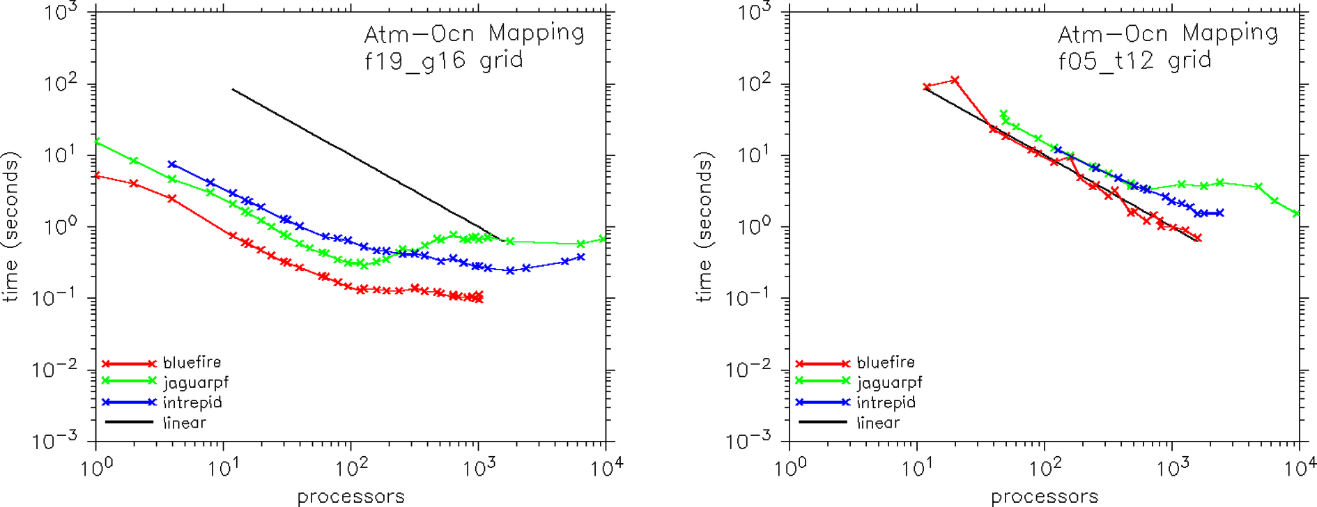
Scaling performance of the atmosphere to ocean mapping kernel in the CCSM4 coupler at two resolutions (‘f19_g16’ and ‘f05_t12’) and on three hardware platforms (bluefire, jaguarpf, and intrepid).
Figure 7 provides some insight into the performance implication of different processor layouts for a specific CCSM coupled run. Figure 7 shows the overall performance of each component schematically for an ‘f19_g16’ moderate resolution fully prognostic case running on a total of 128 processors on bluefire. Figure 7(a) is a fully concurrent layout of components on processors, (b) is a fully sequential layout where all components are run on all processors, (c) is fully sequential except the ocean model is run concurrently with the rest of the system, and (d) is a more general mixed sequential/concurrent layout. In all cases, the total number of processors used is 128 and the idle times, represented by gray boxes, were minimized as much as possible. The total runtime for each of the four configurations is 33.5, 20.8, 21.8, and 19.1 seconds per model day for the (a) concurrent layout, (b) sequential layout, (c) sequential plus ocean concurrent layout, and (d) mixed sequential/concurrent layout, respectively. Except for the (a) fully concurrent layout that has significant idle time because of the sequencing limitations of the atmosphere, land, and ice models in the driver, the total performance of the varied processor layouts is relatively close.
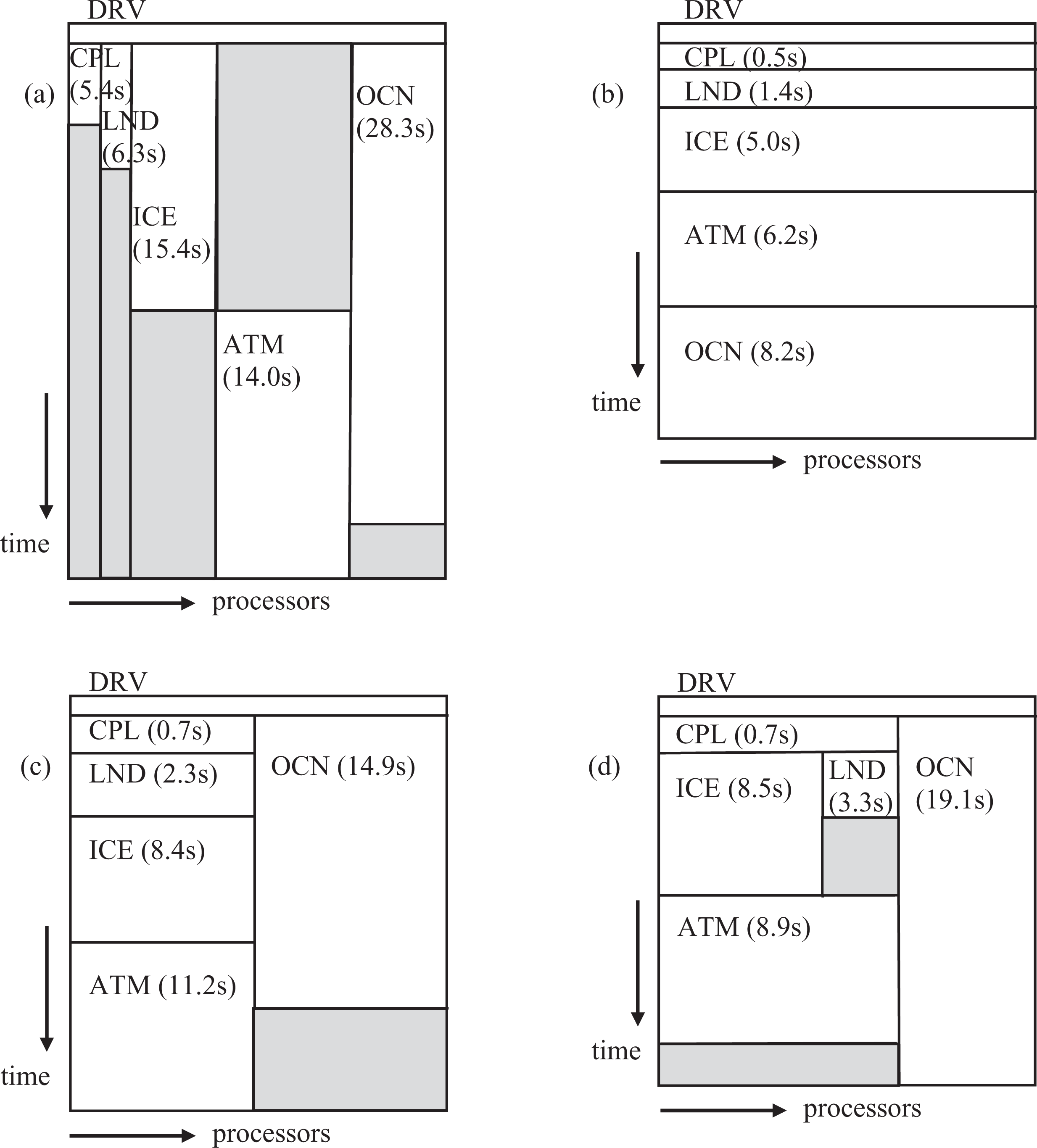
Schematics of CCSM4 component model timing for a fully prognostic ‘f19_g16’ configuration running with four different processor layouts. In all cases, the total number of processors used is 128. Gray boxes represent idle time, and the time for each component in seconds per simulated model day is indicated. The total time for (a) the fully concurrent layout is 33.5 s; for (b) the fully sequential layout is 20.8 s; for (c) the sequential layout with the ocean running concurrently with other components is 21.8 s; and for (d) a mixed sequential/concurrent layout is 19.1 s.
The concurrent layout in Figure 7 cannot be compared to the CCSM3 runtime, because the concurrency is completely different. As was discussed in Section 2, the CCSM3 coupling was implemented with two run phases that allowed greater overlap of work between components. In CCSM4, each component has just one run phase, and this significantly reduces the amount of potential concurrency and increases the runtime of a purely concurrent layout in CCSM4 compared to what would have been attained in CCSM3. However, the increased flexibility of CCSM4 processor layouts generally results in increased performance in nearly all configurations compared to the CCSM3 concurrent-only implementation.
In general, Figure 7 demonstrates some of the potential component layouts on processors available to users of CCSM4. The optimal layout and processor count for each component for any given case depend heavily on the scaling performance of each component and the resolution of each component. In general, the effectiveness of running models concurrently is a trade-off between the idle time created by concurrent execution versus the generally sublinear scaling of components as processor counts are increased.
Since the CCSM3 release, the coupler implementation in the CCSM has been refactored significantly. CCSM4 now contains a top-level driver that calls model component initialize, run, and finalize methods through consistent interfaces. It also coordinates the time sequencing and creation of MPI groups of the components to provide greater flexibility in processor layouts. Many changes were also made to improve the memory and performance scaling of the coupler, and the CCSM4 coupling overhead has been reduced compared to CCSM3. Most of this effort has been implemented using the MCT coupling library. ESMF-compliant interfaces are also available for CCSM4 components.
CCSM4 now scales better to higher processor counts and is able to handle much higher resolution configurations than CCSM3. Scaling curves in CPL6 (Craig et al., 2005) were presented to 32 processors for a T42 (nominally three-degree) atmosphere/land case coupled to a nominally one-degree ocean/ice resolution. In this paper, results are presented for cases up to one-tenth degree global resolutions on processor counts up to 10,000. In particular, CCSM4 has been run with active components at one-quarter degree atmosphere and land global resolutions coupled to a one-tenth degree ocean and ice global resolution (Dennis et al., 2011c). This was not possible with the CCSM3/CPL6 coupling implementation.
The performance of individual coupling kernels has been presented. As expected, trivially parallel operations scale well to high processor counts. In particular, the atmosphere/ocean flux kernel scaled almost linearly on all machines. The memory-intensive merge kernel scaled well, and the communication-intensive rearrange and mapping kernels generally scaled to moderate task counts. Several factors need to be considered when choosing the coupler processor count and layout for overall CCSM4 load balance and performance. The number of operations per timestep in the coupler is generally small compared to other components, and it is often run sequentially with other components, particularly the atmosphere model. As a result, the coupler is often placed on available processors based on load balance and optimization of the other components first. The coupler processor count is generally not the most critical optimization with respect to the overall model throughput. However, based upon the scaling of the communication kernels on jaguarpf, there is the possibility that the coupler performance degrades on some machines as processor counts are increased, so it is important to evaluate the effect of increasing processors on coupler performance before carrying out a long run.
Some general statements could also be made about the relative performance of the different hardware architectures used in this study. On a per processor basis, bluefire was consistently faster than either jaguarpf or intrepid for the coupler timings in general. The memory-intensive merge kernel timings were similar for all machines, especially in the regime where there are many gridcells per processor. However, the computation-intensive flux calculation was 10 times slower on intrepid compared to either bluefire or jaguarpf. This is somewhat expected based on the relative processor speeds. The performance scaling of the communication-intensive kernels on all machines tailed off at higher processor counts, with jaguarpf performing worst at the higher processor counts. It is unclear whether the communication scaling behavior on jaguarpf is inherent to the hardware, associated with the local system setup, or related to the diverse load on the machine at any given time.
Finally, the flexibility to vary the processor layout in CCSM4 has been demonstrated. The CCSM4 model’s ability to support sequential, concurrent, or mixed layouts provides much greater flexibility with respect to overall load balance and performance optimization compared to CCSM3.
Footnotes
The CESM project is supported by the National Science Foundation and the Office of Science (BER) of the US Department of Energy. The NCAR is sponsored by the National Science Foundation. This work has been supported by the Office of Science (BER) US Department of Energy under contracts DE-FC02-97ER62402, DE-FC02-07ER64340 and DE-AC02-06CH11357. Additional support has been provided by the National Science Foundation grant AGS-0856145. This research used resources at the Climate Simulation Laboratory at NCAR’s Computation and Information Systems Laboratory (CISL), sponsored by the National Science Foundation; the Oak Ridge Leadership Computing Facility located in the NCCS at ORNL, which is supported by the Office of Science (BER) of the Department of Energy under Contract DE-AC05-00OR22725; and the Argonne Leadership Computing Facility at ANL, which is supported by the Office of Science of the US Department of Energy under contract DE-AC02-06CH11357