An application-level parallel I/O library for Earth system models

Abstract

We describe the design and implementation of an application-level parallel I/O (PIO) library for the reading and writing of distributed arrays to several common scientific data formats. PIO provides the flexibility to control the number of I/O tasks through data rearrangement to an I/O friendly decomposition. This flexibility enables reductions in per task memory usage and improvements in disk I/O performance versus a serial I/O approach. We illustrate the impact various features within PIO have on memory usage and disk I/O bandwidth on a Cray XT5 system.

Keywords

Parallel I/O Earth System Modeling parallel computing memory efficient netCDF

1 Introduction

For the past 30 years, the amount of computing power that could be applied to scientific problems has grown exponentially. This growth has been achieved both through improvements in single-core performance and the use of parallel processing to perform calculations in parallel. Parallel processing has been enabled by the Message Passing Interface (MPI Forum 1998), a well-accepted and adopted standard for a number years in the scientific software community. A direct result of this growth in computational power is a similar increase in the amount of data generated by scientific simulations. While parallel I/O and file systems have made possible the parallel input and output of data, the maturity and therefore adoption of parallel I/O has lagged behind that of parallel programming. The adoption rate of parallel I/O within large scientific applications has been slow for a number of both technical and sociological reasons, including the diversity of potential I/O needs, the state of parallel file systems, complex user interfaces of parallel I/O software, the industry’s focus on maximizing floating-point rates, and the fact that not all scientific problems require high I/O rates. I/O performance is too frequently an afterthought that only garners attention when it impedes or prevents particular scientific inquiry.

Many of the above reasons were behind the slow adoption of parallel I/O in the Community Earth System Model (CESM; see http://www.cesm.ucar.edu/) (previously known as Community Climate System Model (CCSM)). CESM is a coupled, state-of-the-art global climate model used to study the interaction of the ocean, atmosphere, land, sea ice and other Earth system components. Trends toward larger number of processors with limited memory per core in high-performance computing platforms provided the possibility to significantly increase the resolution of the component models, however the small amounts of memory per core began to conflict with CESM’s previous serial I/O approach.

The CESM code base, which currently consists of five different component models each with a separate 5- to 30-year development history, had a number of different I/O strategies. The Community Atmosphere Model (CAM) (Neale et al. 2010) (the atmosphere component) used a metadata rich NetCDF (Network Common Data Format) format for history files, and it used binary files to provide restart (checkpoint) capability. The Parallel Ocean Program (POP) (Jones et al. 2005; Smith et al. 2010) (the ocean component), the Community Land Model (CLM) (Hoffman et al. 2005) (the land component), the Community Ice CodE (CICE) (Hunke and Lipscomb 2008) (the sea ice component), and the Coupler (CPL) all used various combinations of NetCDF and binary for generating output files. While the POP component did have basic parallel I/O capability for three-dimensional (3D) variables, there was no parallel I/O capability for two-dimensional (2D) variables. Most component models simply collected all data to be written to a single MPI task that then called serial I/O libraries. While such a design may be reasonable for certain combinations of hardware and file systems, it artificially limited the resolutions and core configurations on which the entire model could be run. For example, attempts to use the serial I/O approach within POP on 30,000 Blue Gene/L cores exhausted memory due to message passing buffer allocation issues.

Based on the trends in model resolution and computing hardware, CESM developers decided to introduce a parallel I/O capability into the component models. Our goals were to enable parallel I/O into all component models and achieve the performance advantage potential of general I/O libraries while isolating users from their complexity. The resulting software layer between the applications and general parallel I/O libraries came to be called PIO. Henceforth, we use ‘PIO’ to refer to this new library and ‘parallel I/O library’ to refer to more general-purpose parallel I/O libraries. PIO was therefore designed to address both the needs of several different Earth system component models and the deficiencies in existing parallel I/O libraries.

PIO is not simply an application wrapper library. Instead it is a thin software layer between application code and more generic general-purpose libraries. PIO provides a ‘separation of concerns' to its user. Specifically it separates the concern of the application programmer, who defines what to write/read from disk, from the concern of the I/O library developer, whose focus is how to perform the operation efficiently. While PIO was initially developed to address critical deficiencies in the I/O infrastructure of CESM, the library is sufficiently general and flexible as to be applicable to other scientific disciplines that need to read and write large distributed multi-dimensional arrays.

In Section 2 we describe the design and motivation of the library. In Section 3 we describe key features of the library including how decompositions are described to the library, which is a key difference between PIO and general I/O libraries. In Section 4 we present a comparison of the impact several configurations of PIO have memory usage and disk I/O bandwidths for a single benchmark problem on a large Cray XT5. A rigorous multi-platform comparison of PIO performance is beyond the scope of this paper. We provide conclusions and directions for future work in Section 5.

2 Motivation and design

PIO was designed with the goals of reducing the amount of memory necessary to perform I/O while enabling improved performance versus a serial I/O library. PIO is not a general-purpose I/O library, rather it is an attempt to modify the tradeoffs in ease of use versus complexity that several general-purposes libraries provide. There are a number of general-purpose I/O libraries. MPI-IO (Thakur et al. 1998) is part of the MPI2 standard and defines a large number of interfaces that provide a great deal of flexibility on how to perform I/O. The NetCDF3 and NetCDF4 (Rew and Davis 1990) (see also http://www.unidata.ucar.edu/software/netcdf/) are format standards that are popular within the climate and broader computing community. The NetCDF format provides the ability to include both variables and metadata to describe the included variables. While the NetCDF3 standard stores variables contiguously, the NetCDF4 standard is build on a significantly more flexible HDF5 (see http://hdf.ncsa.uiuc.edu/HDF5) standard. HDF5 uses a block-based file format, and provides explicit support for hierarchical namespaces and data compression. Like NetCDF3, it is used by a broad variety of scientific disciplines.

The ADIOS library (Jin et al. 2008; Lofstead et al. 2009) is a meta I/O library that provides a simplified user interface and flexible support for multiple underlying generic I/O back-ends. ADIOS provides its own parallel BP file format and asynchronous capabilities (Abbasi et al. 2009; Docan et al. 2008). ADIOS does not provide the capability of potentially unique computational and I/O decompositions. This limits its ability to achieve good bandwidth when writing non-rectangular decompositions to a NetCDF file.

Parallel I/O capability was initially achieved within CAM by using ZLIB (Tseng and Ding 2008). Like PIO, ZLIB rearranges 3D variables into an I/O decomposition such that the vertical $z$ dimension is decomposed across cores. While such an I/O decomposition may be ideal for modest levels of parallelism, it does not address the MPI buffering issues that may occur when a large number of cores send messages to a single MPI task. Further, it only provides rearrangements for CAM-specific decomposition.

Several key design principles were used to guide the development of PIO: extensibility, flexibility, ease of use, and backwards compatibility with existing CESM output file formats. The key to PIO extensibility is the ability to utilize different general-purpose libraries as back-end I/O libraries. Currently the supported back-end libraries include MPI-IO, NetCDF3, NetCDF4, and pNetCDF (Li et al. 2003). While HDF5 is not explicitly provided as a back-end in PIO, the NetCDF4 format is based on the HDF5 library.

Flexibility is also a key requirement due to the fact that CESM is a community code with a large user base and a diverse set of scientific interests. Consequently, a single technical solution is not suitable for all users. This can be illustrated by considering the following use cases. User A is running a 32-core job on a 4-node cluster and writing 200 MB files to a Network File System exported from a single server. User B is running on 115,000 cores of a Cray XT writing 100 GB files to a 6 PB Lustre (Sun Microsystems 2007) file system. The correct technical solution for each user is drastically different. While it is possible to provide software patches for the different classes of users, the optimal approach is to create an I/O library that provides the flexibility to adapt to significantly different I/O requirements via runtime parameter settings.

Early work with the MPI-IO library motivated the requirement to create an I/O library that was easy to use. While MPI-IO provides a very high degree of flexibility, it is often difficult to use and, in particular, does not provide a separation of concerns for its users. The application programmer must focus on both what to write and how to write it efficiently. Its complex interface is likely one reason for the slow adoption rate within the scientific applications. As as result, the PIO application programmer interface (API) was designed to be significantly simpler than the MPI-IO API. The PIO API is based on the serial NetCDF interface and is therefore very familiar to those experienced in using the NetCDF interface. While interface restrictions does somewhat limit the library’s flexibility, the limitations do not impact the ability to achieve good read/write performance.

The final key design principle of PIO is that of maintaining backwards compatibility with existing output file formats and structure. The climate community has a large number of tools that are based on processing NetCDF files. Support for efficiently writing and reading NetCDF files is therefore a requirement. The file structure where each component model writes distinct output files is also maintained. There are two possible approaches to generating NetCDF files in parallel: either multiple writers each generate their own file (multiple writer/multiple files) or multiple writers generate a single file (multiple writer/single file). The multiple writer/multiple file approach allows maximum bandwidth but would force changes to the CESM post-processing workflow. Further, manipulation of a large number of smaller files on a parallel file system can be time consuming and have a catastrophic impact on metadata operations (Antypas et al. 2006). A multiple writer/single file approach typically results in lower bandwidth due to lock contention issues among the multiple writers. Currently, PIO only chooses to support the generation of single files, which provides backwards compatibility with the post-processing software. However PIO could be easily extended to support the multiple writer/multiple files approach. While the multiple writer/single file approach does negatively impact achievable bandwidth, the magnitude can be mitigated at the MPI-IO layer through use of collective-buffering algorithms (Liao and Choudhary 2008).

3 Features

We next describe several key features of PIO. PIO has a relatively small number of functions with Fortran interfaces. The API has only 10 main functions involving initialization of the library, file creation, decomposition description, basic read and write, and cleanup. There are an additional 13 utilities functions and a number of NetCDF functions have been simply wrapped. A complete description of the PIO user interface is provided online (see http://code.google.com/p/parallelio/).

3.1 I/O method

PIO enables the selection of I/O method as an argument to the open or create subroutines (PIO_openfile, PIO_createfile). The I/O method corresponds to one of the currently supported formats: binary, NetCDF3, or NetCDF4. Access to binary files is provided in serial by the standard Fortran functions, while parallel access is achieved by using the MPI-IO back-end library. Serial access to NetCDF3 files is provided through the NetCDF3 library, while parallel access is enabled by the pNetCDF library. Both serial and parallel access to NetCDF4 files are provided by the NetCDF4 library. The simple selection of file format and back-end library through the PIO_openfile or PIO_createfile interface enables the necessary flexibility described in Section 2 for a broad community of users. For example, a serial I/O method would be used when the CESM system is run on a single core for development, or if a parallel file system is unavailable. A simple change to a runtime parameter would allow the same files to be read or written by a parallel back-end I/O library.

3.2 Decomposition description

The most distinguishing feature between PIO and other general I/O libraries is the manner in which decompositions are described. PIO provides a subroutine interface, PIO_initdecomp, that specifies how data in memory should be written to or read from disk. In general, the arrangement of data within memory, computational decomposition, is not necessarily optimal for writing to disk, or ‘I/O friendly’. While certain models use a rectangular block decomposition, others use much more specialized decompositions based on computational load balancing. For example, the atmosphere model, CAM, uses a diurnal load-balancing strategy where grid-points from the opposite sides of the Earth are grouped on the same task, whereas the ocean model (POP) and sea-ice model (CICE) use domains that are composites of rectangular blocks.

An example of a possible ocean decomposition is illustrated in the top section of Figure 1 (the computational decomposition). Note that for MPI tasks 0 (PE 0) and 2 (PE 2), the L shaped domain is constructed by combining three square blocks, while the Z shaped domain for PE 1 is constructed of four square blocks. While it is possible to describe the computational domains in Figure 1 using MPI data-types using a single MPI-IO subroutine call, it is not possible using the NetCDF3, NetCDF4, or pNetCDF libraries. The NetCDF libraries only provide the ability to describe domains using a start–count approach. The start–count approach uses two arrays, the count array that describes the size of the rectangular domain to be written, while the start array describes its location within the global index space. It would only be possible to describe the decomposition in Figure 1 to NetCDF libraries using multiple calls to the API; such a call structure has a significant negative impact on read/write performance.

Figure 1.

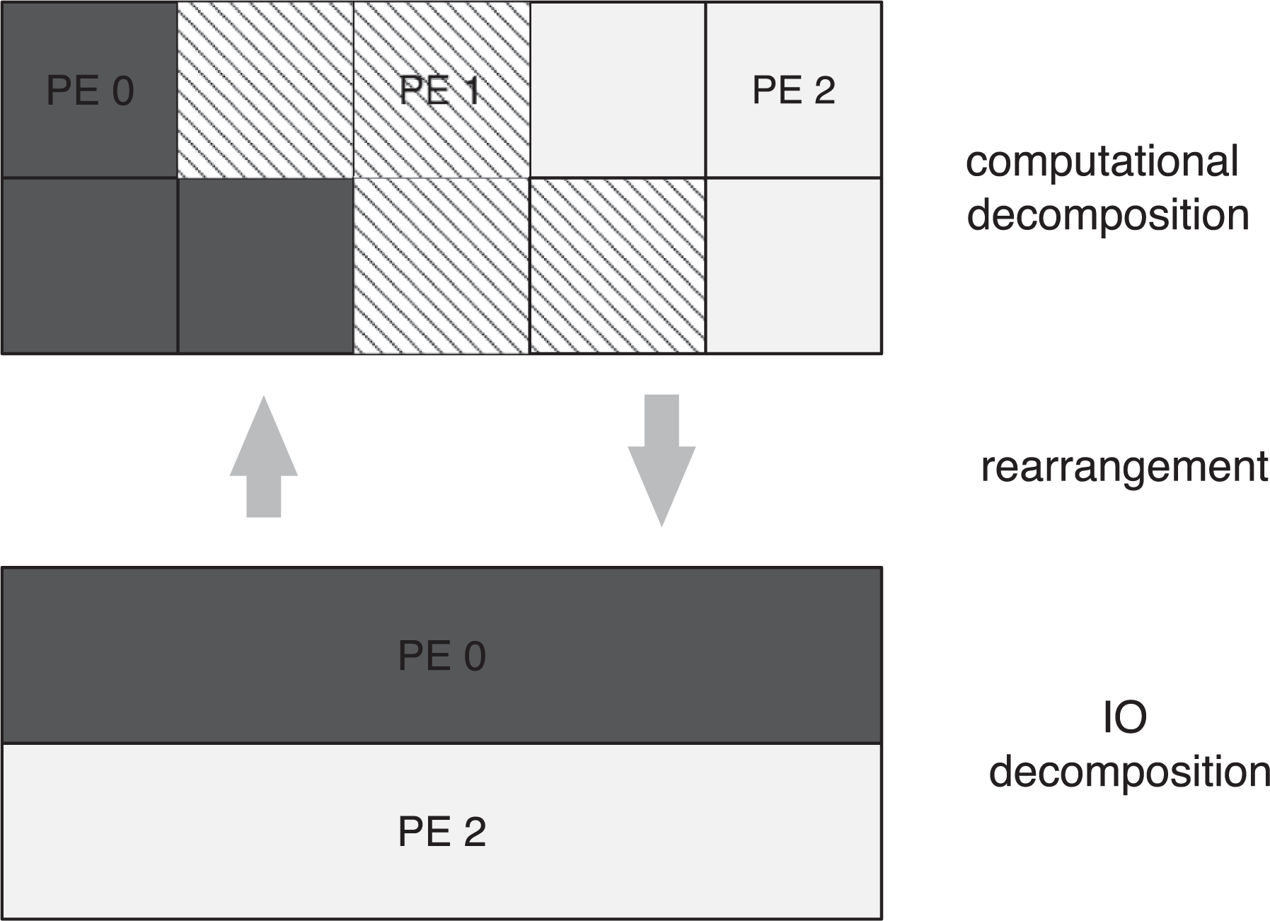
An 2D array that is decomposed across multiple MPI tasks. Note that the computational decomposition is across three MPI tasks, while the I/O decomposition is across two tasks.

PIO addresses the lack of flexibility within the NetCDF libraries by providing the ability to define an I/O decomposition, on the I/O tasks, separate from the computational decomposition which is defined on the computational tasks. While it is possible for the computational decomposition and I/O decomposition to be identical, typically the I/O decomposition is defined on a significantly smaller number of I/O tasks (num_iotasks) than computational tasks. The ability to rearrange data between the computational and I/O decompositions is provided. The bottom section of Figure 1 illustrates a possible I/O decomposition. Note that the data located on PE 1 in the computational decomposition is moved during rearrangement to the PE 0 and PE 2 as part of the rearrangement to the IO decomposition.

The rearrangement that PIO provides is effectively a user-level collective buffering, which is separate from any collective buffering that may be occurring in an underlying MPI-IO layer (Liao and Choudhary 2008; Thakur et al. 1998). PIO provides several versions of the PIO_initdecomp; we first describe the simplest version that mimics the interface used by the NetCDF libraries and then move on to a more complex and flexible interface.

3.2.1 Block-cyclic interface

The block-cyclic version of the PIO_initdecomp subroutine assumes that the arrays are decomposed in a block-cyclic structure and can be described simply using a start–count type approach. A simple block-cyclic decomposition for a 1-dimensional (1D) array is illustrated in the top panel of Figure 2 . We follow the standard FORTRAN 1-based index scheme. Note that contiguous layout of the data in memory can be easily mapped to a contiguous layout on disk. The start argument corresponds to the starting point on disk of the block of contiguous memory, while the count is the number of words. Note that start and count must be arrays of length equal to the dimensionality of the distributed array. While we use a 1D array for simplicity, PIO currently supports up to 5-dimensional (5D) arrays. In the case of 5D arrays, the start and count arrays would be of length five.

Figure 2.

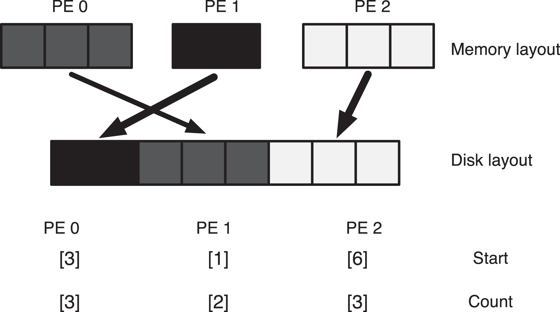
The top panel illustrates the start and count arrays for a single 1D array distributed across three MPI tasks. The bottom panel is the example code for calling the PIO_initdecomp interface from PE 0 to implement the decomposition.

In the bottom panel of Figure 2 is the call to PIO_initdecomp for PE 0 that would be necessary to implement the decomposition illustrated in the top panel. The variable ioSYS is created by the call to PIO_init, a subroutine that initializes the PIO library. The second argument PIO_double is the PIO kind, and indicates that this is a decomposition for an 8-byte real variable. The argument dims is the global dimension for the array. The start and count arrays are 8-byte integers, while iodesc is the IO descriptor generated by the call to PIO_initdecomp.

3.2.2 Degree of freedom interface

The PIO_initdecomp interface described in the previous section mimics the syntax used by both the pNetCDF and NetCDF4 libraries to describe decompositions. However as Figure 1 illustrates, it is insufficient for the more complex decompositions that are frequently used in full scale applications. PIO provides a more general interface to PIO_initdecomp based on the degree of freedom (DOF) concept. Each word within the distributed array is assigned a unique value that corresponds to its ordered placement in the file on disk. So the first word in the file on disk has a DOF of 1, the second 2, etc. This enables a very flexible specification of the decomposition.

This approach is the same as the decomposition description used in the Model Coupling Toolkit (MCT) (Jacob et al. 2005; Larson et al. 2005). The initial development of PIO used MCT to rearrange data between computational and I/O decompositions. MCT, however, was written for a general case where decompositions on each side of the rearrangement are unconstrained. Within PIO, however, the I/O decompositions are restricted to be block-cyclic. This restriction allowed for a faster and simpler ‘box rearranger’ to be developed for use within PIO.

To illustrate the DOF interface, a simple 1D decomposition is illustrated in Figure 3 . Since PE 0 and PE 1 do not contain contiguous pieces of the distributed array, the desired order on disk is specified using the compDOF argument to PIO_initdecomp. In this example, PE 0 contains the 2nd, 4th, and 5th elements of the array, PE 1 contains the 1st and 3rd, and PE 2 contains the 6th, 7th, and 8th elements of the array. The integer compDOF arrays for each MPI task are illustrated at the top of Figure 3. Note that several of the blocks in Figure 3 that represents the I/O decomposition are multicolored (in the online version of this article). The red and yellow blocks correspond to words that were sent from PE 1 to PE 0 during rearrangement. While the yellow and cyan correspond to words that were sent from PE 0 to PE 2. The example code that calls PIO_initdecomp on PE 0 is provided in the bottom of Figure 3. Note that the optional arguments, ioStart and ioCount, specify the I/O decomposition. If these arguments are omitted, PIO will utilize several heuristic algorithms to construct a suitable I/O decomposition.

Figure 3.

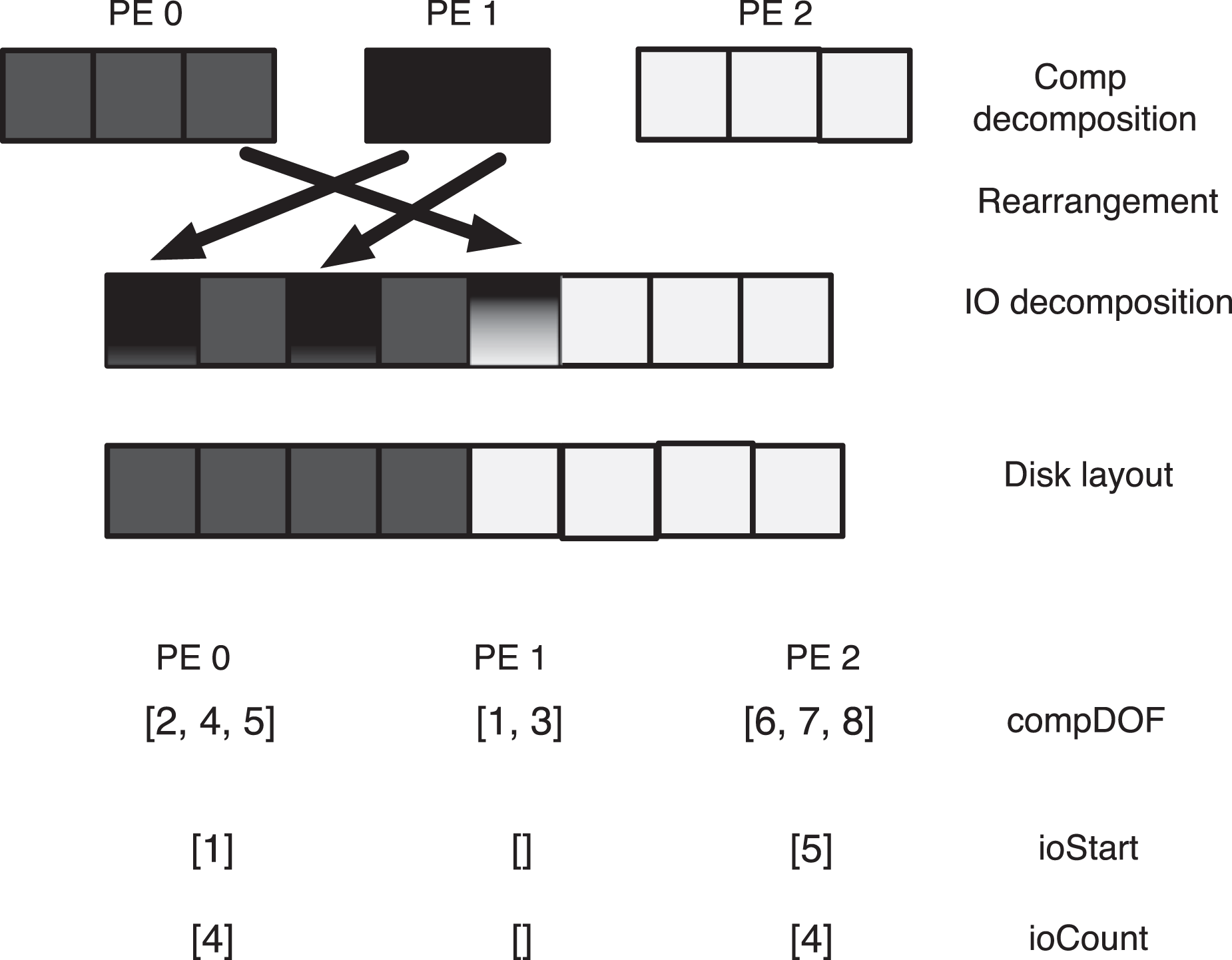
The top panel illustrates a single 1D array distributed across three MPI task and written from two tasks after rearrangement by the box rearranger. The bottom panel is example code for calling the PIO_initdecomp interface from PE 0 to implement the decomposition.

3.3 Flow control

PIO contains a flow algorithm that controls the rate and volume of messages sent to any one destination MPI task. Ideally message passing algorithms should be designed to send a modest number of messages evenly distributed across a number of destinations. Unfortunately, not all message passing algorithms generate well-behaved traffic patterns. A poorly behaved traffic pattern may involve a large number of tasks sending large messages to a single destination task. An excessive number of messages set to a single destination MPI task can exhaust the message passing buffer space available on the destination task. This may cause the application to encounter significant slowdown due to the retransmitting of dropped messages, or at worst complete application failure. In fact, application failure due to insufficient unexpected message buffer space has been a common problem encountered on Cray XT systems. The standard approach has been to tune a large number of environment variables in order to enable the successful writing of output files.

The flow-control algorithm in PIO eliminates resource exhaustion problems by implementing a rendezvous-like protocol that only sends messages when the receiver is ready and has sufficient resources. While the flow-control algorithm may somewhat increase message passing cost when the message passing traffic is well behaved, it significantly reduces costs and increases robustness for poorly behaved traffic patterns.

4 Results

We now illustrate the positive impact of PIO on memory usage and disk I/O bandwidth. We utilize ‘testpio’ an I/O kernel that allows PIO to simulate real I/O patterns used in CESM. We execute ‘testpio’ on Kraken, a 110,000 core Cray XT5 system at the National Institute for Computational Science (NICS). Kraken has a 2.3 PB Lustre parallel file system that provides a theoretical 30 GB s^–1 bandwidth. The file system is constructed of 336 Object Storage Targets (OSTs), each of which is a hardware RAID. Files are written by striping over one or more OSTs. Typically the larger the number of OSTs that are used, the higher the potential write bandwidth. However, using a large number of OSTs, also increases the probability of encountering large variations in file system performance. For this study we choose to stripe over a total of 16 OSTs. We examine the impact that number of OSTs has on variability for a single configuration in Section 4.2.

For this discussion, we use the POPD benchmark configuration where PIO reads and writes variables of size 1.3 GB. This benchmark represents the I/O traffic generated by the POP ocean model at 0.1° when writing or reading a 3D array of 3600×2400×40 4-byte reals. A total of 10 variables are written to and read from 10 separate NetCDF or binary files. We examine the maximum memory per MPI task and I/O bandwidth for a number of PIO configurations associated with core counts ranging from 64 to 15,000. Note that the core counts in Figure 4 refer to the number of MPI tasks used for the computational decomposition. Because there is a large amount of variability in the file system performance on Kraken (Dennis and Loft 2009), a busy shared resource, the maximum sustained disk I/O bandwidth obtained for a single file is reported. In Section 4.2 we demonstrate that the maximum sustained disk I/O bandwidth is a reasonable approximation for what is observed on average.

Figure 4.

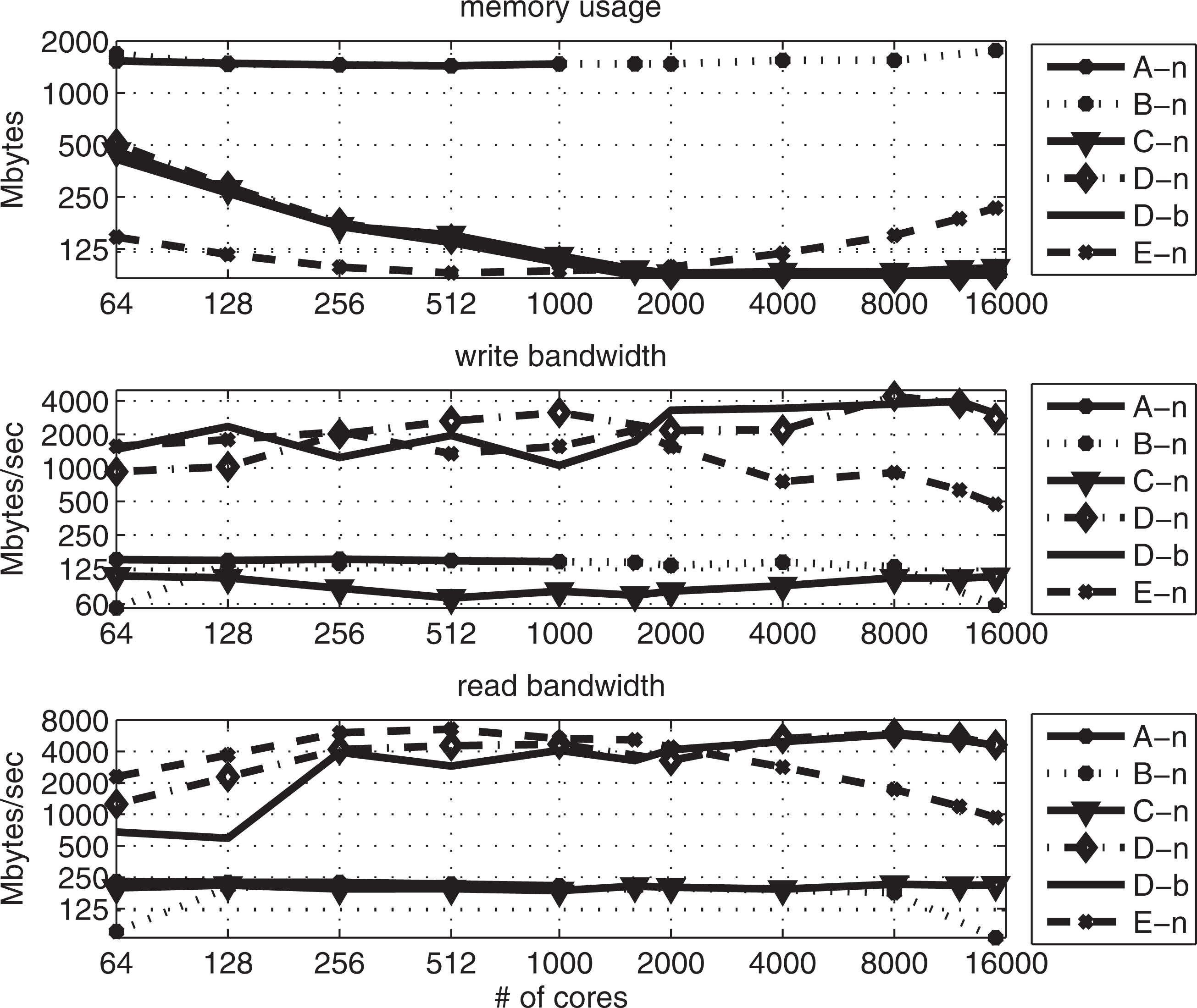
Characteristics of POPD benchmark on Kraken using the PIO configurations described in Table 1. The top panel represents the maximum memory usage per MPI task. The middle panel is the maximum write bandwidth. The bottom panel is the maximum read bandwidth.

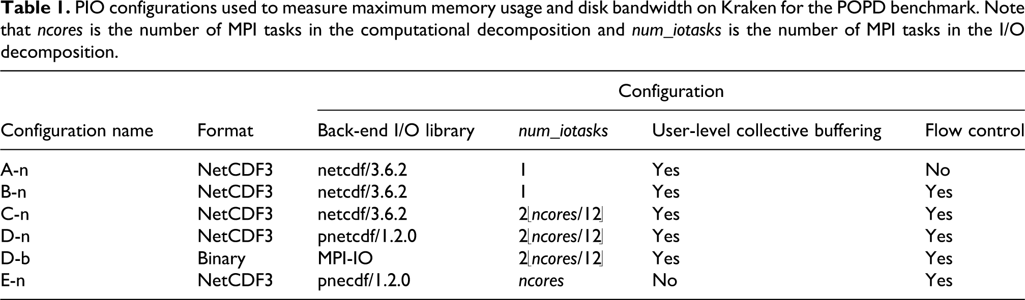
4.1 Impact of different PIO configurations

The different PIO configurations are described in Table 1 and involve different settings for file format, the back-end I/O library, the number of iotasks (num_iotasks), and use of user-level collective buffer and flow-control. Configuration names are constructed using capital letters (A, B, C, D, and E), followed by a hyphen and either n or b indicating NetCDF or binary files, respectively. While we focus on NetCDF I/O, a single binary configuration is included in order to evaluate potential impact of file formats. Note that only the A-n configuration, which involves tuning off the flow-control algorithm within PIO, requires recompilation. This configuration is not used in practice, but is presented here for pedagogical purposes. The remaining five configurations only involve changes to input namelist files.

Table 1.
PIO configurations used to measure maximum memory usage and disk bandwidth on Kraken for the POPD benchmark. Note that ncores is the number of MPI tasks in the computational decomposition and num_iotasks is the number of MPI tasks in the I/O decomposition.

Configuration

Configuration name Format Back-end I/O library num_iotasks User-level collective buffering Flow control

A-n NetCDF3 netcdf/3.6.2 1 Yes No

B-n NetCDF3 netcdf/3.6.2 1 Yes Yes

C-n NetCDF3 netcdf/3.6.2 2〈ncores/12〉 Yes Yes

D-n NetCDF3 pnetcdf/1.2.0 2〈ncores/12〉 Yes Yes

D-b Binary MPI-IO 2〈ncores/12〉 Yes Yes

E-n NetCDF3 pnecdf/1.2.0 ncores No Yes

		Configuration
A-n	NetCDF3	netcdf/3.6.2	1	Yes	No
B-n	NetCDF3	netcdf/3.6.2	1	Yes	Yes
C-n	NetCDF3	netcdf/3.6.2	2〈ncores/12〉	Yes	Yes
D-n	NetCDF3	pnetcdf/1.2.0	2〈ncores/12〉	Yes	Yes
D-b	Binary	MPI-IO	2〈ncores/12〉	Yes	Yes
E-n	NetCDF3	pnecdf/1.2.0	ncores	No	Yes

In order to simulate the characteristics of serial I/O traffic prior to the introduction of PIO, the testpio POPD benchmark is configured to use the serial NetCDF3 library and a single IO-task and the PIO flow-control algorithm is disabled. The memory usage and bandwidths obtained using this configuration A-n are illustrated in Figure 4. As expected the maximum memory usage is significant in the configuration A-n, and is 1.4–1.5 GB regardless of number of computational cores used. Attempts to execute the testpio POPD benchmark using configuration A-n on greater than 1000 cores was not possible due to job failure from insufficient MPI unexpected message buffer space. As mentioned previously, this type of failure is a common occurrence when executing poorly behaved message passing traffic patterns on Cray XT systems. The read and write bandwidth for configuration A-n typically varies between 100 and 134 MB s^–1.

Configuration B-n evaluates the impact of the flow-control algorithm. We enable flow control within PIO but otherwise use the same settings as configuration A-n (i.e. the serial NetCDF3 library and a single I/O task). The maximum memory usage and bandwidths for configuration B-n are provided in Figure 4. The memory usage for B-n is similar to A-n for core counts up to 1000 and less for greater than 1000. These results demonstrate that the activation of the PIO flow-control algorithm eliminates the need to tune the MPI environment variables on the Cray XT system in order to write output files. The bandwidths for the POPD benchmark for configuration B-n vary between 95 to 125 MB s^–1. The impact multiple I/O tasks has on memory usage and bandwidth is described next.

As mentioned in Section 3.2, PIO provides the user with the capability to vary the number of IO tasks (num_iotasks). In configuration C-n we vary num_iotasks by setting the number of iotasks to be approximately twice the number of nodes used by each job. However, we still utilize the serial NetCDF3 library. In this configuration PIO avoids the memory needed by the previous configurations by sending and writing each cores data in turn instead of gathering an entire field before writing. Because Kraken has 12 cores per node, num_iotasks = 2 〈ncores/12〉 where ncores is the number of cores. As can be seen in Figure 4, C-n dramatically reduces the maximum memory when compared with the previous two configurations. Maximum memory is only 460 MB on 64 cores and drops to 97 MB on 15,000 cores. While read disk bandwidths for the C-n configuration is slightly improved to between 140 and 200 MB s^–1 depending on core count, the write disk bandwidths drop slightly to 70–120 MB s^–1.

The previous three configurations used the serial NetCDF3 back-end library. We next quantify the impact the use of a parallel back-end library has on the POPD benchmark. The D-n and D-b configurations use the pNetCDF and MPI-IO back-end library, respectively. Both configurations use the same number of num_iotasks as in the configuration C-n. As expected the maximum memory usage for both the D-n and D-b configurations is very similar to the C-n configuration and decreases with increasing core count. The impact in disk I/O bandwidth between the serial and parallel back-end libraries is dramatic. The write bandwidth for both the D-n and D-b vary between approximately 925 MB s^–1 on 64 cores to 4.4 GB s^–1 on 2000 cores. Configurations D-n and D-b also achieve excellent read bandwidths that vary from 675 MB s^–1 on 64 cores to 5.9 GB s^–1 on 8000 cores. The very similar performance results for the D-n and D-b configurations, particularly at large core counts, illustrate that there is no significant performance impact imposed by the NetCDF standard versus an MPI-IO generated binary file.

Due to the particular decomposition used by the ‘testpio’ code for the POPD benchmark, which can be described using the start–count approach, it is possible to evaluate the impact rearrangement within PIO has on memory usage and bandwidth. We affectively disable user-level collective buffering when we configure PIO to not perform rearrangement. In the E-n configuration, all MPI tasks call the back-end pNetCDF library. As Figure 4 illustrates, the E-n configuration enables significant reductions in the maximum memory per MPI task for fewer than 1600 cores. For greater than or equal to 1600 cores the per core memory usage is greater than the C-n, D-n, or D-b configurations that utilize user-level rearrangement. In particular, the maximum memory usage of 215 MB observed on 15,000 cores is twice as large.

4.2 Impact of file system variability

Variability in file system performance can be considerable due to interference with other users (Dennis and Loft 2009). We next examine the impact of file system variability observed on Kraken for our ‘testpio’ code for the POPD benchmark. Recall for the previous section that ten variables are written to and read from ten separate NetCDF or binary files. Figure 4 contains the maximum rates for a single file. We illustrate the observed variability for all six PIO configurations on 1000 cores in Figure 5 . In Figure 5 the rates for all 10 files are provided along with lines that represent the minimum, maximum, and average write rates in the top panel, and read rates in the bottom panel. Interestingly, the A-n configuration shows no significant difference between its minimum and maximum write and read rates and is the only configuration which does not use the flow-control algorithm. The write rates for the B-n, C-n configurations, which use a serial back-end library, show modest variability, while the D-n, D-b, and E-n configurations, which use a parallel back-end library, show considerable variability. For example the maximum write rates for the D-n configuration is 9.7 times larger than the minimum write rate. Fortunately, the average write rate suggests a large percentage of the maximum write rate is achieved in practice.

Figure 5.

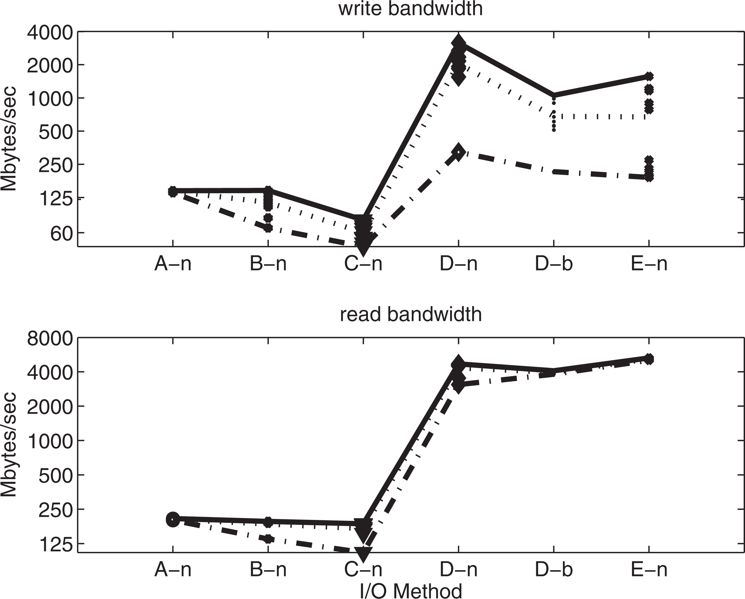
Performance variability for POPD benchmark on 1000 cores of Kraken using the PIO configurations described in Table 1. The top panel represents the write bandwidth. The bottom panel is the read bandwidth.

We next examine the impact that the number of OSTs has on variability of read and write rates. Using the D-n configuration on 1000 cores we vary the number of OSTs which PIO uses from 4 to 144. Note that 144 is the maximum number of IO tasks that PIO will use for the POPD benchmark on 1000 cores. The write and read rates are provided in Figure 6 . Note that a large degree of variability in I/O performance is apparent regardless of the number of OSTs. The most severe variability in write performance is observed for 64 OSTs, where the maximum rate of 1030 MB s^–1 is 50 times faster than the minimum rate of 20 MB s^–1. A similarly large spread in maximum to minimum performance is observed on 8 OSTs. While the maximum read rate occurs for 16 OSTs, it should be noted that is likely a consequence of running the benchmark on a busy shared resource. Figure 6 clearly illustrates that there is no compelling reason to utilize more than 16 OSTs when running the POPD benchmark in the D-n configuration on 1000 cores of Kraken.

Figure 6.

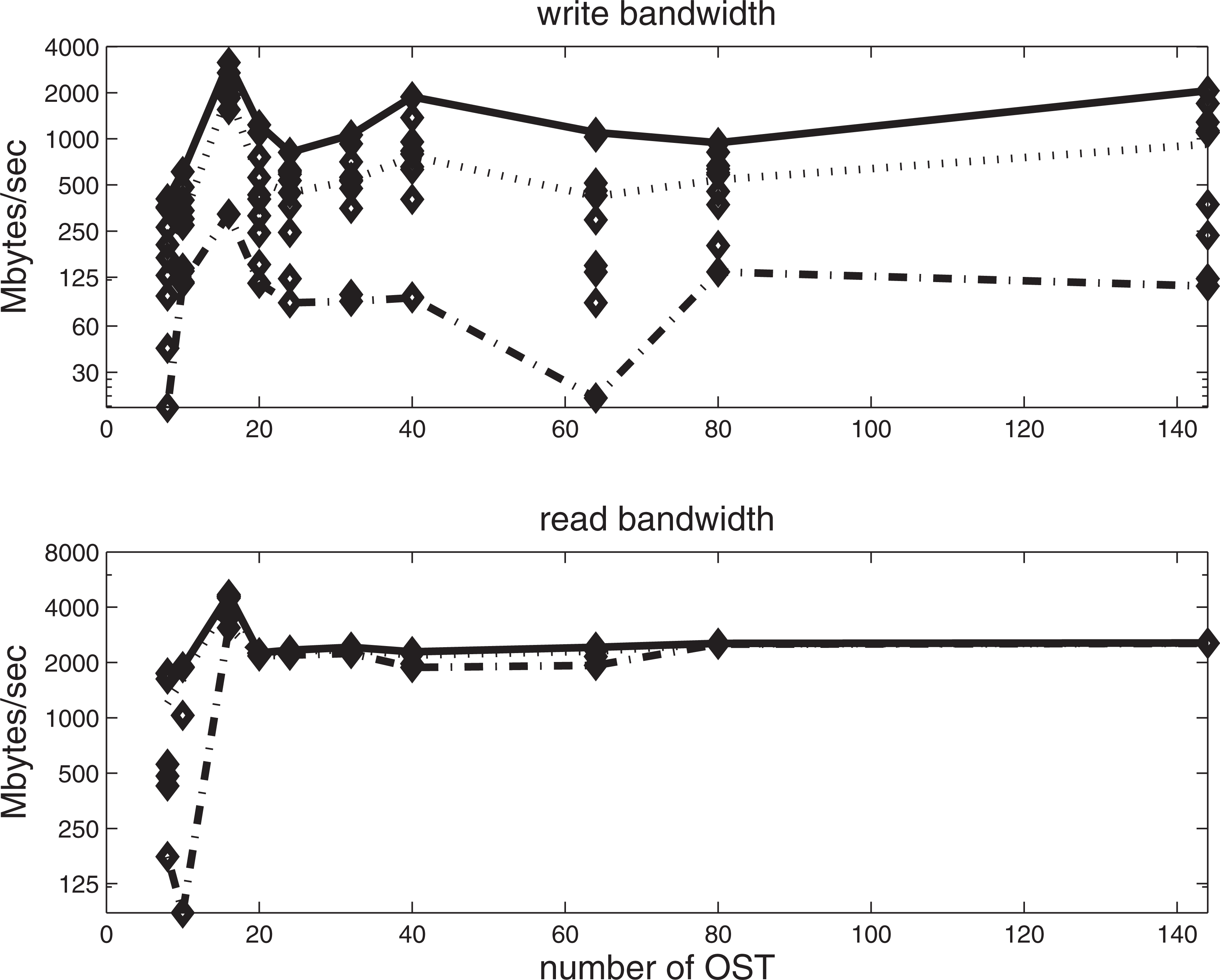
Performance variability for POPD benchmark using D-n configuration on 1000 cores of Kraken for different number of OSTs. The top panel represents the write bandwidth. The bottom panel is the read bandwidth.

5 Conclusion and future work

In this paper we have described an application-level parallel I/O library (PIO) that enables the reading and writing of distributed arrays to common scientific data formats. It represents a compromise between flexibility and ease of use that is missing among the general-purpose I/O libraries. PIO was designed to be flexible, easy to use, without sacrificing the ability to achieve good I/O bandwidth. While PIO was initially designed to satisfy the needs of several earth systems models, its interface is sufficiently general to allow it to be used by a number of scientific disciplines that need to write distributed multi-dimensional arrays.

We have demonstrated the impact that several key features of the library have on the maximum per MPI task memory usage, and read and write bandwidths on a large Cray XT5 system. In particular, we demonstrated how flow-control improves PIO’s robustness. We have also demonstrated that the user-level collective buffering within PIO allows maximum memory usage to scale with core count resulting in a significant reduction in memory usage. The impact of the memory reduction has already had a positive impact on the scientific capability of CESM. For example, one configuration of CESM that uses a 0.125° atmosphere model was unable to even read in its initial condition data without the memory-saving features of PIO. A 0.25° configuration of CAM with 399 chemical tracers could not output its data without PIO. We also demonstrated that it is possible to significantly increase disk I/O bandwidth through use of the parallel I/O back-end libraries.

There are a number of opportunities for future work As alluded to earlier in the paper, we intend to provide a rigorous evaluation of performance on several different compute platform and file system combinations including IBM Blue Gene/P, IBM POWER6, and Cray XT. This evaluation will involve looking at other benchmarks besides the POPD benchmark described in this paper. We are also actively collaborating with developers of the Vapor Project (Clyne et al. 2007; Clyne and Rast 2005) to add a parallel wavelet compression capability within PIO.

Footnotes

Acknowledgments

We would like to thank Rob Ross and Rob Latham of Argonne National Laboratory for numerous discussions concerning the design and implementation of the library. We would also like thank Pat Worley of Oak Ridge National Laboratory for implementing the flow-control algorithm, Matthew Woitaszek of the National Center for Atmospheric Research and Kate Ericson of Colorado State University for help optimizing the library on Blue Gene optimizations, and Nathan Hearn and Michael Arndt of the National Center for Atmospheric Research for performance investigations on the Cray XT, and improvements to the memory usage. PIO has matured significantly due to feedback from early users including the developers of CESM as well as Samson Cheung of National Atmospheric and Space Administration.

This work was financially supported by the National Science Foundation (Cooperative Grant NSF01 that funds the National Center for Atmospheric Research [NCAR], and grant numbers OCI-0749206, CCF-0937939, OCE-0825754, and AGS-0856145). Additional funding is provided through the Department of Energy, Office of Biological and Environmental Research (grant numbers DE-FC02-97ER62402 and DE-FC02-07ER64340) and Climate Change Prediction Program (Program Grant DE-PS02-07ER07-06) and the DOE Scientific Discovery through Advanced Computing Program (grant number DE-FG02-06ER06-04). Work on the part of AA Mirin was performed under the auspices of the US Department of Energy by Lawrence Livermore National Laboratory (contract number DE-AC52-07NA27344). This manuscript has been created in part by Argonne National Laboratory and the Argonne Leadership Computing Facility, which are supported by the Office of Science of the US Department of Energy (contract number DE-AC02-06CH11357).

References

Abbasi

Wolf

Eisenhauser

Klasky

Schwan

Zheng

(2009) Datastager: Scalable data staging services for petascale applications. In Proceedings of HPDC, pp. 39–48.

Antypas

Calder

Dubey

Fisher

Ganapathy

Gallagher

(2006) Scientific applications on the massively parallel BG/L machines. In Proceedings of PDPTA 2006, pp. 292–298.

Clyne

Mininni

Norton

Rast

(2007) Interactive desktop analysis of high resolution simulations: application to turbulent plume dynamics and current sheet formation. New J Phys 9: 301.

Clyne

Rast

(2005) A prototype discovery environment for analyzing and visualizing terascale turbulent fluid flow simulations. In Proceedings of Visualization and Data Analysis 2005.

Dennis

Loft

(2009) Optimizing high-resolution climate variability experiments on the Cray XT4 and XT5 systems at NICS and NERSC. In Cray User Group (CUG09), Atlanta, GA.

Docan

Parashar

Klasky

(2008) Enabling high speed asynchronous data extraction and transfer using DART. In Proceedings of the 17th International Symposium on High-Performance Distributed Computing (HPDC), Boston, MA. Los Alamitos, CA: IEEE Computer Society Press.

Hoffman

Vertenstein

Kitabata

White

JB III

(2005) Vectorizing the Community Land Model. Int J High Perform Comput Appl 19: 247–260.

Hunke

Lipscomb

(2008) CICE: the Los Alamos sea ice model documenation and software user’s manual version 4.0. Technical Report LA-CC-06-012, Los Alamos National Laboratory, T-3 Fluid Dynamics Group.

Jacob

Larson

Ong

(2005) MxN compunication and parallel interpolation in CCSM3 using the Model Coupling Toolkit. Int J High Perform Comput Appl 19: 293–307.

10.

Jin

Klasky

Hodson

Lofstead

Abbasi

. (2008) Adaptive IO System (ADIOS). In Cray User Group (CUG08).

11.

Jones

Worley

Yoshida

White

JB I

Levesque

(2005) Practical performance portability in the Parallel Ocean Program (POP). Concurrency Comput Pract Exper 17: 1317–1327.

12.

Larson

Jacob

Ong

(2005) The Model Coupling Toolkit: A new fortran90 toolkit for building multiphysics parallel coupled models. Int J High Perform Comput Appl 19: 277–292.

13.

Liao

Choudhary

Ross

Thakur

Gropp

. (2003) Parallel netCDF: A high-performance scientific I/O interface. In In Proceedings of the ACM/IEEE Conference on Supercomputing (SC).

14.

Liao

Choudhary

(2008) Dynamically adapting file domain partitioning methods for collective I/O based on underlying parallel file system locking protocols. In In Proceedings of the ACM/IEEE Conference on Supercomputing (SC), pp. 313–344.

15.

Lofstead

Zheng

Klasky

Schwan

(2009) Adaptable, metadata rich IO methods for portable high performance IO. In In Proceedings of IPDPS’09, Rome, Italy.

16.

MPI Forum (1998) MPI-2: a message passing interface standard. High Performance Computing Applications 12: 1–2.

17.

Neale

Richter

Conley

Park

Lauritzen

Gettelman

(2010) Description of the NCAR Community Atmsophere Model (CAM 4.0). Technical Report NCAR/TN-???+STR, National Center for Atmospheric Research.

18.

Rew

Davis

(1990) The unidata netCDF: Software for scientific data access. In Sixth International Conference on Interactive Information and Processing Systems for Meteorology, Oceanography, and Hydrology. Anaheim, CA: American Meteorology Society, pp. 33–40.

19.

Smith

Jones

Briegleb

Bryan

Danabasoglu

Dennis

. (2010) The Parallel Ocean Program (POP) reference manual: Ocean component of the Community Climate System Model (CCSM). Technical Report LAUR-10-01853, Los Alamos National Laboratory.

20.

Sun Microsystems (2007) Lustre file system: High-performance storage architecture and scalable cluster file system. http://whitepapers.zdnet.com/abstract.aspx?docid=349537.

21.

Thakur

Gropp

Lusk

(1998) Data sieving and colletive I/O in ROMIO. In Proceedings of the Seventh Symposium on the Frontiers of Massively Parallel Computation. Los Alamitos, CA: IEEE Computer Society Press, pp. 182–189.

22.

Tseng

Ding

(2008) Efficient parallel I/O in Community Atmosphere Model (CAM). Int J High Perform Comput Appl 22: 206–218.

		Configuration
Configuration name	Format	Back-end I/O library	num_iotasks	User-level collective buffering	Flow control
A-n	NetCDF3	netcdf/3.6.2	1	Yes	No
B-n	NetCDF3	netcdf/3.6.2	1	Yes	Yes
C-n	NetCDF3	netcdf/3.6.2	2〈ncores/12〉	Yes	Yes
D-n	NetCDF3	pnetcdf/1.2.0	2〈ncores/12〉	Yes	Yes
D-b	Binary	MPI-IO	2〈ncores/12〉	Yes	Yes
E-n	NetCDF3	pnecdf/1.2.0	ncores	No	Yes