A Partitioned Global Address Space implementation of the European Centre for Medium Range Weather Forecasts Integrated Forecasting System

Abstract

Today the European Centre for Medium Range Weather Forecasts (ECMWF) runs a 16 km global T1279 operational weather forecast model using 1536 cores of an IBM Power7. Following the historical evolution in resolution upgrades, the ECMWF could expect to be running a 2.5 km global forecast model by 2030 on an exascale system that should be available and hopefully affordable by then. To achieve this would require the Integrated Forecasting System (IFS) to run efficiently on about 1000 times the number of cores it uses today. In a step towards this goal, the ECMWF have demonstrated the IFS running a 10 km global model efficiently on over 40,000 cores of HECToR a Cray XE6 at the Edinburgh Parallel Computing Centre. However, getting to over a million cores remains a formidable challenge, and many scalability improvements have yet to be implemented. The ECMWF is exploring the use of Fortran2008 coarrays; in particular, it is possibly the first time that coarrays have been used in a world-leading production application within the context of OpenMP parallel regions. The purpose of these optimisations is primarily to allow the overlap of computation and communication, and further, in the semi-Lagrangian advection scheme, to reduce the volume of data communicated. The importance of this research is such that if these and other planned developments are successful, the IFS model may continue to use the spectral transform method to 2030 and beyond on an exascale-sized system. The current status of the coarray scalability developments within the IFS are described together with a brief outline of future developments.

Keywords

PGAS Fortran2008 Coarrays

1. Introduction

The Integrated Forecasting System (IFS) is the European Centre for Medium Range Weather Forecasts’ (ECMWF’s) production application used to provide medium-range weather forecast products up to 10 or 15 days ahead to its Member States and Co-operating States. At shorter range, national weather services use products from the ECMWF to provide boundary data for their own regional and local short-range forecast models. Figure 1 shows the evolution of the IFS model from the mid-1980s to the current T1279 operational model and extrapolated out to 2030. Figure 1 shows that halving the horizontal grid spacing has occurred about every 8 years, and provides an estimate for the dates when the T3999 (~5 km) and T7999 (~2.5 km) models could be introduced into operation. It is clear that this simplistic extrapolation (given the number of grid columns and slope from T106 to T1279) does not take into account the many architectural and technology changes that are needed to get to the exascale.

Figure 1.

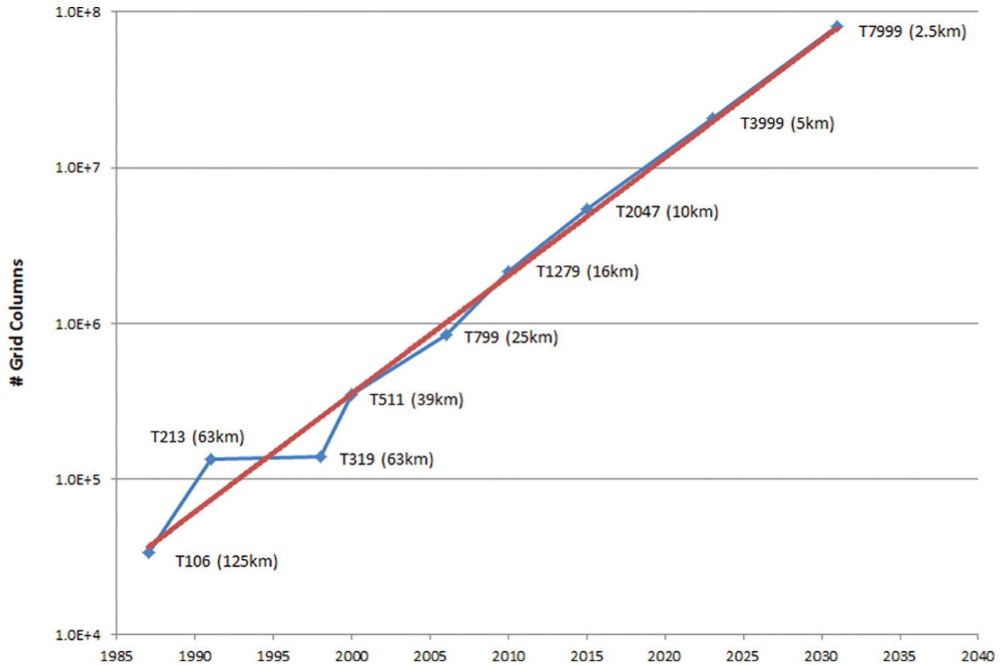
Evolution of the Integrated Forecasting System (IFS) model, showing that the IFS resolution, measured here in the number of grid columns and corresponding grid-point distances, halves approximately every 8 years.

The ECMWF is an application partner in a European Union (EU)-funded project called CRESTA (Collaborative Research into Exascale Systemware, Tools and Applications) bringing the IFS numerical weather prediction application to the project. For the IFS the initial focus of developments in CRESTA is primarily to use Fortran2008 coarrays (ftp://ftp.nag.co.uk/sc22wg5/N1801-N1850/N1824.pdf) within OpenMP parallel regions to overlap computation with communication and thereby improve performance and scalability. Fortran2008 coarrays is an implementation of the Partitioned Global Address Space (PGAS) programming model (http://en.wikipedia.org/wiki/Partitioned_global_address_space). This research is significant as the techniques used should be applicable to other hybrid Message Passing Interface (MPI)/OpenMP codes with the potential to overlap computation and communication. Of course, using coarrays is not a panacea to get codes to achieve scaling at the exascale. What it does allow us to do is to experiment with exposing parallelism at the fine scale for both computation and communication. It is expected that future developments to the IFS will build on this work. One of the challenges of the CRESTA project is to think more disruptively and we may consider more innovative approaches; for instance, to run component models in parallel and explore Direct Acyclic Graph (DAG) scheduling (Bosilca et al., 2012).

The IFS is a spectral transform (Temperton, 1991), semi-implicit (Temperton et al., 2001), semi-Lagrangian (SL; Ritchie et al., 1995) weather prediction code, where model data exists in three spaces, namely, Fourier, spectral and grid-point space. In a single time step (Figure 2) data is transposed between these spaces so that the respective grid point, Fourier and spectral computations are independent over two of the three coordinate directions in each space (Barros et al., 1995). For example, in grid-point space computations are independent over the horizontal domain (latitudes and longitudes), but dependent over the vertical levels. Likewise, in spectral space (Legendre transform), computations are independent over zonal wave numbers and levels, but dependent on total wave numbers.

Figure 2.

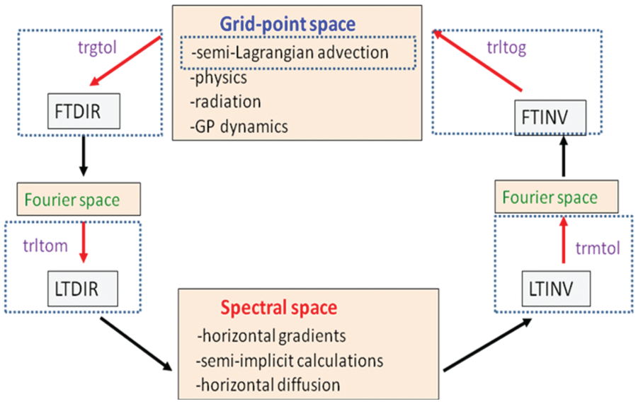
Integrated Forecasting System (IFS) time step: in a single time step IFS data is transformed starting from grid-point space to Fourier space then to spectral space and back to Fourier space and finally to grid-point space. This diagram shows areas of IFS optimisation (the dotted boxes) where a coarray optimisation has been applied. In grid-point space we have optimised the SL advection scheme. In the four other areas of optimisation, we have optimised a data transposition routine (beginning with letters ‘tr’) with the associated computational routine. These are the pairs trgtol:FTDIR, trltom:LTDIR, trmtol:LTINV and trltog:FTINV. The optimisation essentially replaces the MPI communication done in the associated ‘tr’ routine with coarray (PGAS) communication in the context of the OpenMP work loop where the computation is done. The computation routines are either Fourier transforms, where overlap is done at the granularity of a latitude, or Legendre transforms, where overlap is done at the granularity of zonal wave numbers.

Fourier transforms (boxes labelled FTINV and FTDIR) are performed between grid-point and Fourier space, and Legendre transforms (boxes labelled LTINV and LTDIR) are performed between Fourier and spectral space. A full description of the above IFS parallelisation scheme is contained in Barros et al. (1995).

At the ECMWF, this same model is used in an Ensemble Prediction System (EPS) suite where today 51 models are run at lower resolution with perturbed input conditions to provide probabilistic information to complement the high-resolution forecast. The EPS suite is a perfect candidate to run on future exascale systems, with each ensemble member being independent. By increasing the number of members and their resolution it is relatively easy to fill a future exascale system. However, at the same time there will be a need to perform model simulations at convection-resolving resolutions of O(1 km), which is more challenging to scale.

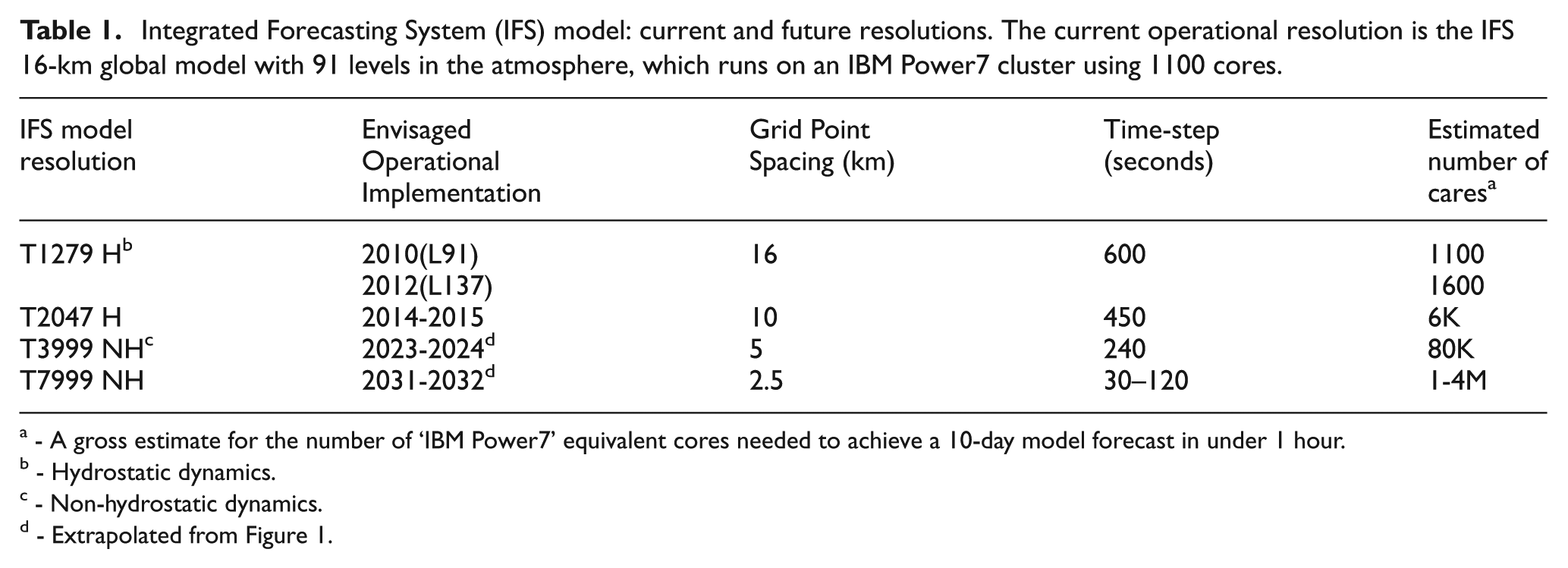
Today the ECMWF uses a 16 km global grid for its operational high-resolution model, and plans to scale up to a 10 km grid in 2014–2015, followed by further resolution increases, as shown in Table I. These model resolution increases will require the IFS to run efficiently on over a million cores by around 2030.

Table 1.

Integrated Forecasting System (IFS) model: current and future resolutions. The current operational resolution is the IFS 16-km global model with 91 levels in the atmosphere, which runs on an IBM Power7 cluster using 1100 cores.

IFS model resolution	Envisaged Operational Implementation	Grid Point Spacing (km)	Time-step (seconds)	Estimated number of cares^a
T1279 H^b	2010(L91)2012(L137)	16	600	11001600
T2047 H	2014-2015	10	450	6K
T3999 NH^c	2023-2024^d	5	240	80K
T7999 NH	2031-2032^d	2.5	30–120	1-4M

- A gross estimate for the number of ‘IBM Power7‘ equivalent cores needed to achieve a 10-day model forecast in under 1 hour.

- Hydrostatic dynamics.

- Non-hydrostatic dynamics.

- Extrapolated from Figure 1.

The IFS comprises several component suites, namely, a 10-day high-resolution forecast, a four-dimensional variational analysis (4D-Var), an EPS and an ensemble data assimilation system (EDA). For the CRESTA project it has been decided to focus on the IFS model to understand its present limitations and to explore approaches to get it to scale well on future exascale systems. While the focus is on the IFS model, it is expected that developments to the model should also improve the performance of the other IFS suites (EPS, 4D-Var and EDA) mentioned above.

The resolution of the operational IFS model from 2010 to 2013 was T1279L91 (1279 spectral waves and 91 levels in the atmosphere). For the IFS model, it is paramount that it completes a 10-day forecast in less than one hour so that forecast products can be delivered on time to ECMWF member states. The IFS model is expected to increase in resolution over time, as shown in Table I. As can be seen in this table, the time-step reduces as the model resolution increases. For the IFS, halving the grid spacing typically increases the computational cost by 12; a factor of 2 for each of the horizontal coordinate directions, a factor of 2 for halving the time step and only 50% more for the increase in vertical levels. However, in reality the cost can be greater than this, when items are included such as the Legendre transforms and Fourier transforms that increase the cost non-linearly.

It is clear from this that the IFS model from a computational complexity viewpoint can utilise future supercomputers at the exascale and beyond. What is less clear is whether the IFS model can continue to run efficiently on such systems and continue to meet the operational target of one hour when running on 100,000 or more cores, which it would have to do. The performance of the IFS model has been well documented over the past 20 years, with many developments to improve performance, with more recent examples described by Mozdzynski (2006, 2008), Salmond (2008), Hamrud (2010), Salmond and Hamrud (2010) and Mozdzynski (2014). In recent years focus has turned to the cost of the Legendre transform, where the computational cost is O(N**3) for the global model, where N denotes the cut-off wave number in the triangular truncation of the spherical harmonics expansion.

This has been addressed by a Fast Legendre Transform (FLT) development, where the computational cost is reduced to C_L *N**2*log(N), where C_L is a constant and C_L <<N. The relative performance improvement is shown in Figure 3, where the matrix–matrix multiply routine dgemm is the cost of the original algorithm and FLT is the cost of the new algorithm. It should be noted that the FLT algorithm is only used for wave numbers beyond 1279, even within higher resolution models. The FLT algorithm is described by Rokhlin and Tygert (2006), Tygert (2008, 2010) and Wedi et al. (2013). While the cost of the Legendre transforms has been addressed, the associated TRMTOM and TRMTOL transpositions (also shown in Figure 2) between Fourier and spectral space remain relatively expensive at T3999 (>10% of wall time). Today, these transpositions are implemented using efficient MPI_alltoallv collective calls in separate communicator groups, which can be considered the state of the art for MPI communications. In addition, the cost of transpositions between grid-point space and Fourier space are also relatively expensive, these being TRGTOL and TRLTOG, and are implemented today by non-blocking MPI_send, MPI_recv and MPI_wait calls as no MPI collective calls are applicable here. Figure 4 shows the relative cost of the spectral method for current and planned IFS resolutions as run on ECMWF’s current IBM Power7 systems. Some of the costs clearly come from increased resolution and the need to use greater numbers of cores. The cost is approximately halved for all resolutions when the hydrostatic version of the model is used (cf. Wedi et al., 2013).

Figure 3.

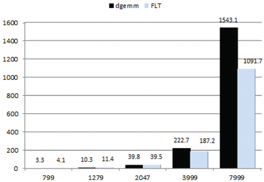
Average wall-clock time compute cost [milliseconds] per spectral transform, where dgemm represents the old algorithm and FLT (Fast Legendre Transform) the new algorithm.

Figure 4.

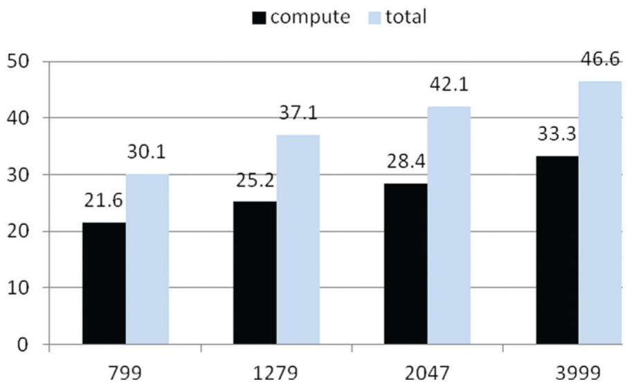
Relative cost of the Integrated Forecasting System spectral method (all 91 levels, all non-hydrostatic (NH) for comparison). This chart shows that the relative cost of the spectral method increases with model resolution. The difference between column pairs is MPI communication, which has the potential to be overlapped with the compute sections of the spectral method, which comprises the Fourier transforms and Legendre transforms.

In Figure 4, the light bars indicate the total cost including the MPI communications involved. Percentages have been derived considering all grid-point dynamics and physics computations but without considering Input/Output (IO), synchronisation costs (barriers) and other ancillary costs. All runs show that the MPI communications cost (the difference between the two columns) is less than or equal to the compute cost on the IBM Power7, providing enough potential for ‘hiding’ this overhead.

In the following sections the current status of the coarray scalability developments to IFS will be presented, including an outline of planned developments.

2. Legendre and Fourier transforms

Within the CRESTA project we are addressing the performance issues described above by using Fortran2008 coarrays (ftp://ftp.nag.co.uk/sc22wg5/N1801-N1850/N1824.pdf, last accessed 07/03/2014) to overlap these communications with the computations in the Legendre and Fourier transforms. Use of coarray syntax allows one-sided transfers to or from remote MPI tasks (called images in coarray syntax) using a simple square bracket syntax extension introduced in the Fortran2008 standard. For the Legendre transforms these transfers are being done for each wave number within an OpenMP parallel region. Figure 5 shows the original and new approaches for the inverse Legendre transform. In the original (OLD) approach the computation (LTINV) and communication (TRMTOL) are done sequentially, with no overlap. In the NEW scheme (using coarrays) each thread is computing and then communicating its computed data to the respective tasks of its ‘communicator’ group. While Fortran2008 has no coarray groups/teams construct it is nevertheless trivial to compute a mapping to a set of image numbers.

Figure 5.

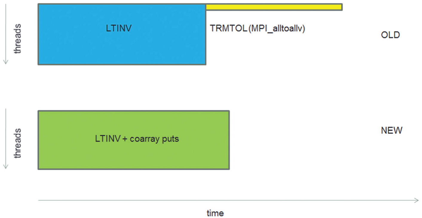
Schematic showing the new overlap of the inverse Legendre transform (LTINV) computations with the associated TRMTOL transposition. In the coarray scheme the same data that was communicated with an MPI_alltoallv is now communicated using coarray puts within an OpenMP loop as results from each iteration of the loop are completed.

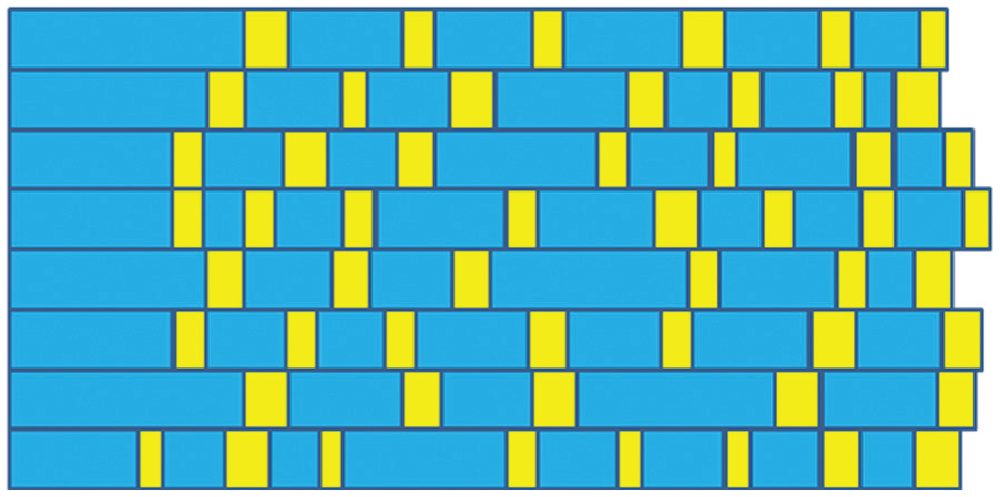
Figure 6 shows how the computation and coarray communication would work in practice, showing work done by eight OpenMP threads. The expectation here is that compute (LTINV, blue-dark) and communication (coarray puts, yellow-light) overlap in time. Experience has shown that the Cray DMAPP library is not thread safe with the Cray Compilation Environment (CCE) version 8.0.6 and earlier releases, and a temporary workaround has been used to locate coarray transfers in OMP CRITICAL SECTIONs with a small performance penalty. The coarray puts are non-blocking, and only waited on for completion on a subsequent SYNC IMAGES statement. For the direct Legendre transforms a similar approach is used. Here the coarray gets in each thread are blocking until data arrives and then progress onto computation. In the above description we have focused on the Legendre transform and the PGAS approach to overlap computation with communication, by performing these in a single OpenMP parallel region that operates over spectral wave numbers. For the Fourier transforms a similar scheme is employed, but instead of spectral wave numbers, the Fourier transforms operate over latitudes, where tasks in Fourier space have a subset of latitudes and a subset of atmospheric levels. The TRGTOL and TRLTOG transpositions (as shown in Figure 2) move data from grid-point space that has a EQ_REGIONS partitioning (Leopardi, 2006; Mozdzynski, 2008), shown in Figure 7, which shows an example of partitioning for 1024 tasks. EQ_REGIONS partitioning is the scheme used in the IFS to partition grid space to MPI tasks. The algorithm results in a partition at each of the poles, and an increasing number of partitions in each band progressing to the equator. Each partition has an equal number of grid points. For the TRGTOL and TRLTOG transpositions data must be communicated to/from MPI partitions that own some number of complete latitudes (subset of levels) to MPI partitions that own some number of part latitudes (all levels).

Figure 6.

Schematic showing the new Integrated Forecasting System approach where inverse Legendre transform computations (blue-dark) are overlapped with the associated TRMTOL transposition (coarray puts, yellow-light).

Figure 7.

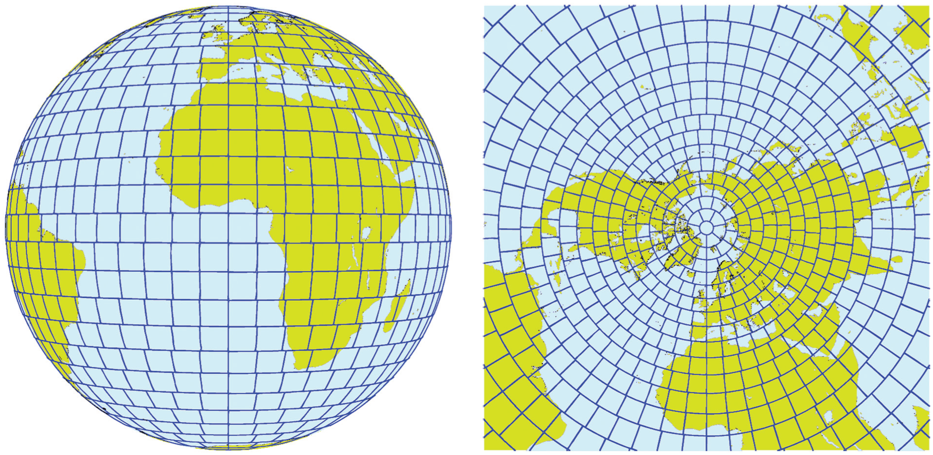
EQ_REGIONS partitioning of grid-point space, showing a partition at the poles and then an increasing number of partitions as we approach the equator.

3. Semi-Lagrangian transport

3.1. Original semi-Lagrangian scheme

The semi-implicit (Temperton et al., 2001) SL (Ritchie et al., 1995) scheme in the IFS allows the use of a relatively long time step compared with an explicit Eulerian time-stepping scheme. This SL scheme (as shown in Figure 8) involves the use of a halo of data from neighbouring MPI tasks, which is needed to compute the departure-point and mid-point of the wind trajectory for each grid point (‘arrival’ point) in a task’s MPI partition, and the interpolation of variables at the departure and mid-point. While the communications in the SL scheme are relatively local, the downside is that the location of the departure point is only known at run time and therefore the IFS must assume a worst case geographic distance for the halo extent, computed from a maximum assumed wind speed of 400 m/s and the time step. Today, each task must perform MPI communications for this halo of data before the iterative scheme can execute to determine the departure-point and mid-point of the wind trajectory. This approach is clearly non-scaling, as the same halo of data must be communicated independent of the size of the grid partition. To address this non-scaling issue, the SL scheme has been optimised to use Fortran2008 coarrays to only get grid columns from neighbouring tasks as and when they are required in the iterative scheme to compute the departure-point and mid-point of the trajectory (using an eight-point stencil), and also for any other grid columns needed for the subsequent interpolations (using a 32-point stencil).

Figure 8.

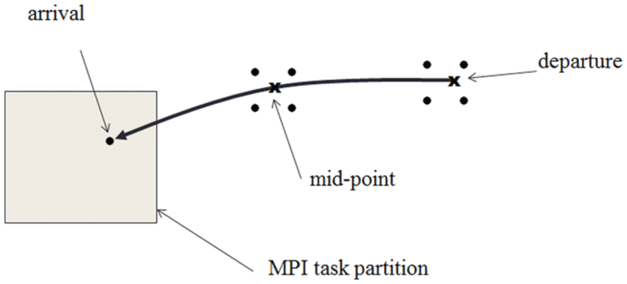
Semi-Lagrangian transport, where the Integrated Forecasting System requires each grid point in a MPI task partition (the arrival point) to determine where that particle of air came from (the departure point) backwards in time . Interpolations are performed at the departure point and the mid-point of the trajectory and data quantities updated at the arrival point.

Figure 9 highlights (in black) the grid points owned by the MPI task that encountered the highest wind speed (120 m/s) during a 10-day forecast starting 15 October 2005. Figure 9 shows a halo of grid points (marked blue-lighter shade) whose width is determined by a maximum wind speed of 400 m/s × the time step (720 s in this case), resulting in a halo distance of 288 kilometres. Only the three wind vector variables u, v, w are obtained from neighbouring tasks for computing the trajectory. The rest of the variables (26) are obtained in the locality of each task, but only for the grid points (grey-lightest shaded area in Figure 10) that have been identified as needed during the process of computing the trajectory, which may be called the on-demand scheme. The SL interpolations can now be performed.

Figure 9.

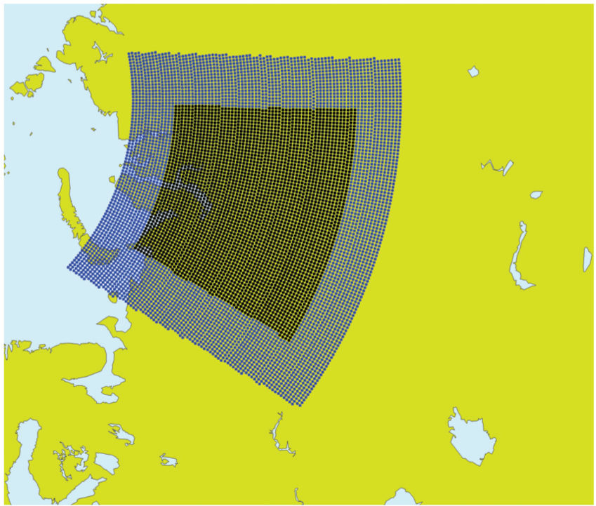
Original semi-Lagrangian transport, showing the max wind halo (blue-lighter shaded area), which is filled with data (wind vector variables u, v, w) from neighbouring MPI tasks. This data is used in the process to compute the departure and mid-points of air particles arriving at task 11’s grid points (black-darker shaded area).

Figure 10.

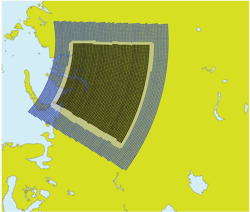
Original semi-Lagrangian transport, showing the halo grid points (grey-lightest shaded area) that are actually used by task 11 for determining the departure and mid-points for all variables. This shows that only a small amount of the max wind halo is actually used and this is for the partition that encountered the highest wind speed.

3.2. PGAS semi-Lagrangian scheme

For the PGAS implementation, only the halo grid points that are used (red-lighter shaded area in Figure 11) are communicated by Fortran2008 coarray transfers. No maximum wind halo is needed with this approach, with a saving on the volume of data communicated, and the number of MPI tasks that need to be communicated with for the SL scheme. To achieve this we have to allocate a coarray SL data structure that duplicates the original SL buffer; however, the dimensions of this coarray need to be transposed such that the leading dimension allows for large contiguous coarray transfers. In Section 5.2 we propose some future work where the SL buffer is itself transposed where the leading dimension would match that of the SL coarray. This would further improve performance as the initialisation of the SL coarray would involve only contiguous memory copies. After SL buffer data is copied into the coarray we need to execute a SYNC IMAGES statement, which is needed before we can access remote coarrays. The remaining code is located in a routine where we compute stencils for the SL scheme. For each stencil point we check a logical array to see if that stencil point is firstly in the halo area and secondly whether it has already been copied from a remote image. If a stencil point is in the halo area and not already copied, then we copy it to the SL buffer and mark the stencil point logical as ‘copied’. The original SL scheme required two OpenMP loops, one OpenMP loop for the determination of the trajectory and a second OpenMP loop for subsequent interpolations. In between the two loops are MPI calls to obtain data from neighbouring tasks. In the PGAS SL scheme only one OpenMP loop is required, which is a merge of the original two loops, with a small improvement in performance due to improved caching of data.

Figure 11.

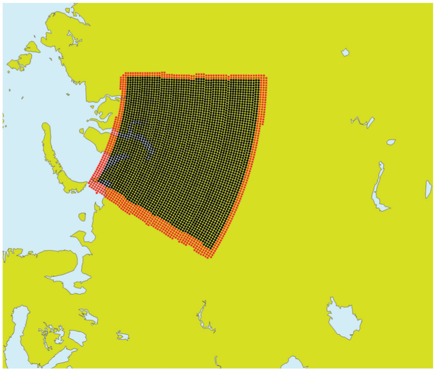
New Partitioned Global Address Space (Fortran2008 coarray) semi-Lagrangian transport, showing the grid points owned by task 11 (black-darker shaded area) and the halo points that are actually used (red-lighter shaded area). With the one-sided coarray approach, we only get data from the halo area when it is needed in the determination of the trajectory and subsequent interpolations.

4. Integrated Forecasting System performance measurements

For an IFS model execution it is crucial that an operational 10-day forecast is completed in under one hour wall time, which is equivalent to 240 forecast days per day (FD/D). Figure 12 shows the performance achieved in April 2012. The latest benchmark release of the IFS, called RAPS12 (corresponding to an ECMWF internal source cycle 37R3), was chosen for runs on HECToR, a Cray XE6, having the Gemini interconnect and Interlagos AMD cores (32 per node). The CCE version was 7.4.4 at the time.

Figure 12.

Performance of the T2047 (~10 km) model with 137 vertical levels using the benchmark RAPS12 Integrated Forecasting System release (CY37R3) on HECToR (Cray XE6), Cray Compilation Environment = 7.4.4, in April 2012.

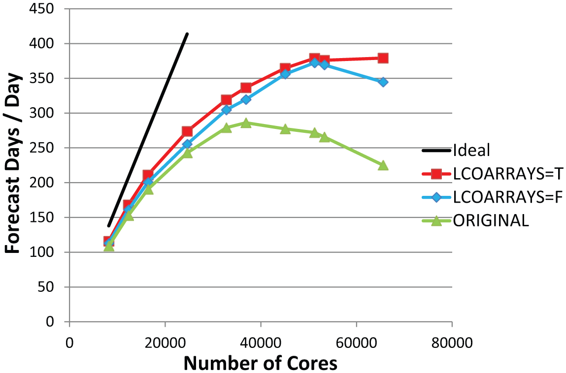
4.1. T2047L137 hydrostatic model

The performance was first measured without any source modifications on up to 64K cores and reached asymptotic performance of 280 FD/D at around 30K cores. With the CRESTA optimisations performance was significantly improved with asymptotic performance of 350 FD/D at around 50K cores. These optimisations included both MPI optimisations (labelled LCOARRAYS=F) and the Legendre transform coarray optimisations (labelled LCOARRAYS=T) described in Section 2, which also included the MPI optimisations. In Figure 13 we show the performance gain from using all the coarray optimisations enabled at run time by namelist setting LCOARRAYS=true. The coarray optimisations are those described earlier in Sections 2 and 3 in the three functional areas, namely, Legendre transforms, Fourier transforms and SL. The runs in Figure 13 were performed using an updated CCE 8.0.6 release, which was both more performant and reliable, now achieving over 500 FD/D on about 50K cores. It should be noted that this level of performance is in excess of two times the requirement for a T2047L137 operational forecast of 240 FD/D.

Figure 13.

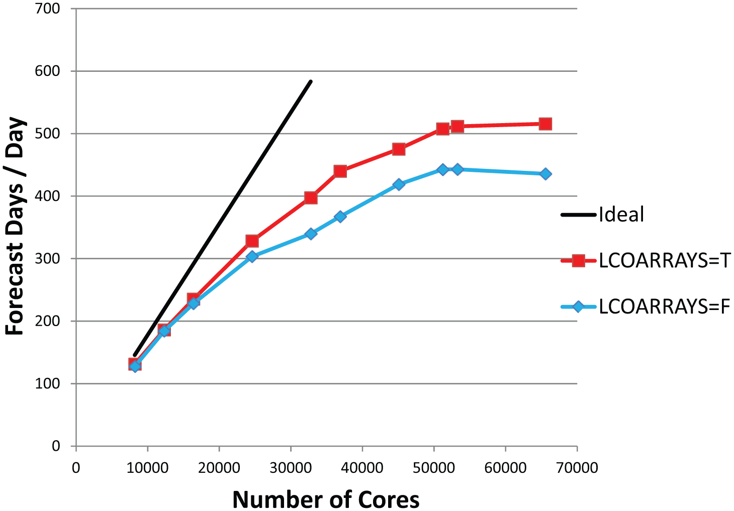
Performance of the T2047 (~10 km) model with 137 levels using the benchmark RAPS12 IFS release (CY37R3) on HECToR (Cray XE6), as before but updated compiler version to Cray Compilation Environment = 8.0.6, in September 2012.

In Figure 14 we show the performance improvement from the coarray optimisations, which peak at 21% at around 40K cores then dip about 5% after this. An analysis of the detailed timers in the IFS (called the gstats package) suggests that rather than the coarray optimisation degrading after 40K cores, the MPI code improved relative to the coarray code. This was evident by inspecting the gstats counters that timed sections of code where MPI calls have been replaced by coarray transfers. The relative slowdown of the coarray version was reproducible and at several nearby core counts (the group of three core counts in Figure 13). It will be interesting to see how the coarray optimisations perform when we run a larger T3999 case (1Q2013/RAPS13/38R2) where there will be greater opportunity for overlap between computation and communication at that resolution, as shown in Figure 5. In Figure 15 we present the efficiency of the T2047L137 IFS model as run on HECToR for the runs described earlier. The efficiency is derived relative to the performance of a single core, which is assumed to be 100% efficient. The single core performance is itself extrapolated from a least squares fit (Excel’s LINEST function) of FD/D performance in the 8–36K core range where the fit is good for all three sets of runs. This figure shows overall efficiency gains of 10% at 8K cores to about 20% at 40–50K cores.

Figure 14.

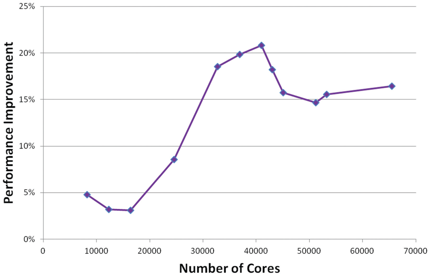
Performance improvement of the T2047 (~10 km) model with 137 levels by using Fortran2008 coarrays on HECToR (Cray XE6).

Figure 15.

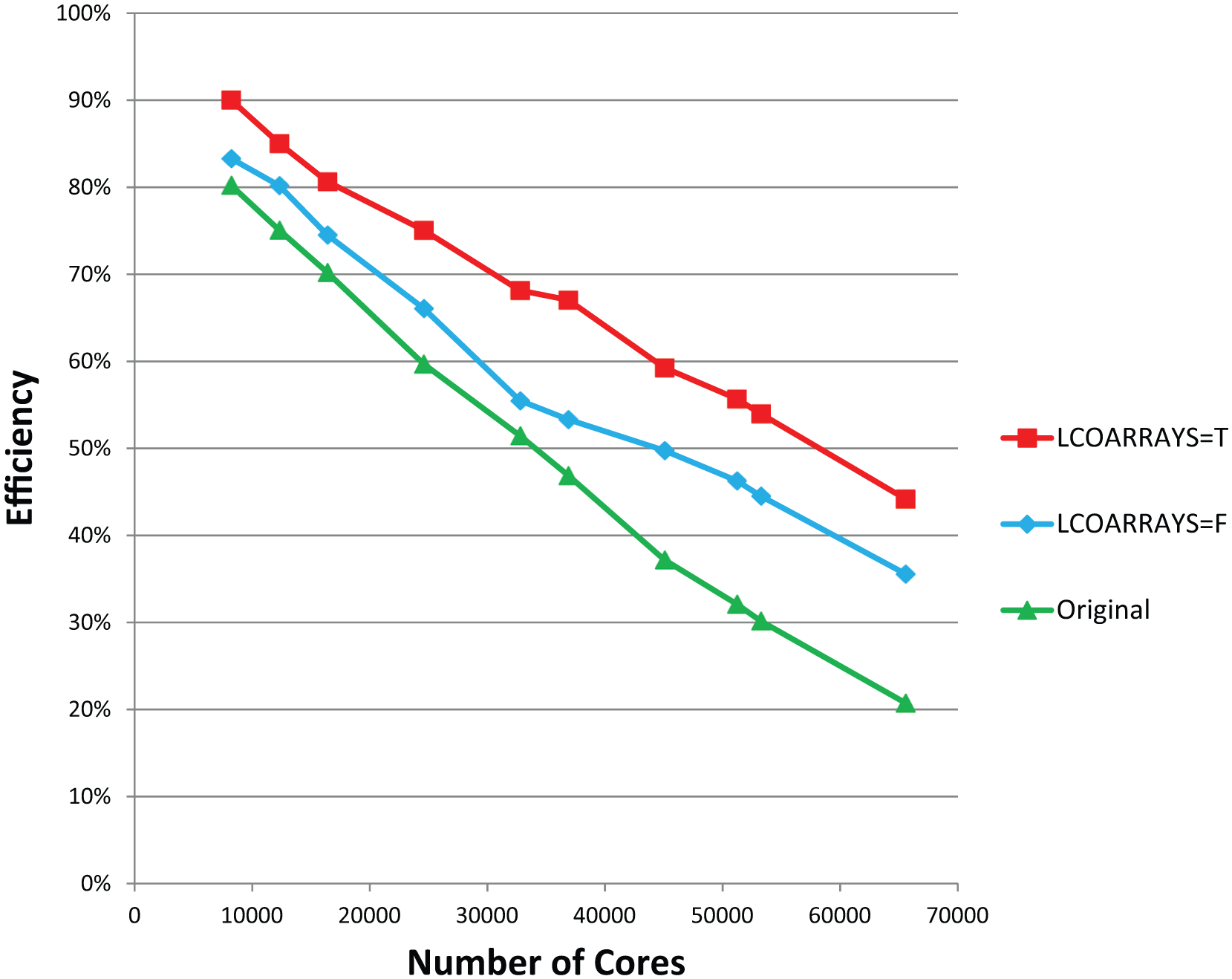
Efficiency of the T2047 (~10 km) model with 137 levels on HECToR (CRAY XE6).

4.2. T2047L137 non-hydrostatic model

The performance of a T2047/L137 NH case is shown in Figure 16. As this case was a 10-km model it did not require NH dynamics but was run solely to observe the effect of the coarray optimisations. Analysis of the performance statistics showed that the relatively expensive NH spectral space computations were scaling poorly. This was due to the fact that the OpenMP parallelism in the spectral computations was limited to 2048 (waves 0–2047) spread across all MPI tasks. In spectral space data is distributed over MPI tasks in a two-dimensional scheme over spectral waves and atmospheric levels. However, the spectral space semi-implicit calculations require access to all atmospheric levels, which require additional data transpositions called TRMTOS and TRSTOM. The scaling issue was resolved by moving the OpenMP parallelisation down one level, where the parallelism would now be min(tasks, 2048) × min(threads, atmospheric levels) or practically 2048 × 8 = 16K, so an eight-fold increase in parallelism. Of course, in the future we could increase the number of threads to 16 and beyond to exploit more parallelism in the spectral computations. This optimisation (50+ OpenMP loops parallelised) resulted in an overall 10% improvement at 45K cores. In the limit the thread-level parallelism in the spectral computations is the product of the number of spectral waves by the number of atmospheric levels, which for a T7999L400 model would be 3.2 million. The performance advantage of using coarrays in this NH dynamics case is now 26%. At resolution T2047 we do not need to run with NH dynamics, but it confirms that the IFS with NH dynamics works with coarrays and prepares for the larger T3999 NH case.

Figure 16.

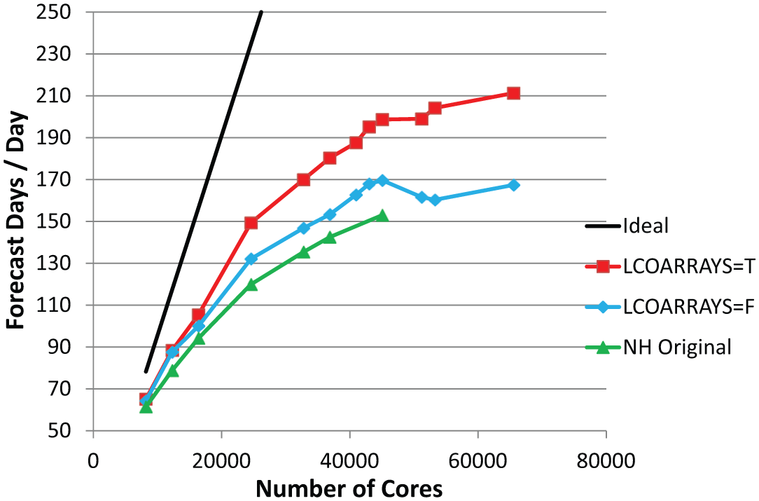
Performance of the T2047 (~10 km) model with 137 levels non-hydrostatic RAPS12 Integrated Forecasting System (CY37R3) forecast model performance on HECToR (Cray XE6), Cray Compilation Environment = 8.0.6, November 2012.

5. Summary and future work

The ECMWF IFS model has been enhanced to use Fortran2008 coarrays to overlap computation and communication in the context of OpenMP parallel regions. This has been applied to the Legendre transforms, Fourier transforms and the SL scheme. This approach has resulted in an overall 20% performance improvement for a T2047L137 10-km model at 40K cores on HECToR, a Cray XE6. In addition to this improvement, a further 20–30% improvement has been made by a combination of MPI optimisation and, in the case of a NH model, by optimising the spectral computations. We expect that the work completed in the first year of three in the CRESTA project has enabled IFS to run at the petascale. A greater challenge remains to enable the IFS for the exascale. A number of optimisations described below may be pursued. However, it is clear that continuous investment into the scalability of the IFS is paramount for the future success of the ECMWF.

5.1. Use of coarray teams

The next Fortran standard (beyond Fortran2008) is expected to support a feature called coarray teams. An issue with the present Fortran2008 standard is that coarrays when allocated must be the same size on each image and the allocation takes place on all images. This behaves like a global operation, something that we want to avoid as we progress to the exascale. In the next standard we will be able to allocate a coarray team, where the size of images across teams can be different and also the allocation of coarrays in teams is independent of such allocations on other teams. With respect to the IFS, this will be more consistent with the IFS parallelisation scheme in Fourier and spectral spaces, and permit the use of dynamic allocation of coarrays in these spaces. Today we minimise the cost of a global coarray allocation by only allocating when a current coarray is too small, and never deallocating it, which is clearly not satisfactory.

5.2. Reorganisation of semi-Lagrangian data structures

The present dominant data structure in the IFS SL scheme is organised such that the leading dimension is a slab, a number of consecutive grid points of full or part latitudes, which include a halo of points obtained from near neighbour tasks. The other non-leading dimension in this data structure is fields, which is a number of variables and their levels. This is not ideal for two reasons; firstly, the ‘max-wind by time-step’ halo can be relatively large at scale and only partially used leading to poor memory scaling, Secondly, for an efficient coarray implementation we need to obtain a full column (fields) of data (many thousands of words) with a single coarray transfer, so the coarray implementation today requires a transpose of the data to be efficient. Both these issues can be resolved by reorganising the data structure with the leading dimension as columns, which will both improve memory scalability and remove the need for transposing the data.

5.3. T3999 non-hydrostatic model

In this paper we have used a 10-km T2047L137 IFS model with hydrostatic dynamics as an example problem. This resolution is destined for operational use in 2015 and will be run at the ECMWF on the replacement high-performance computing system to the current IBM Power7. The first model resolution that may require NH dynamics is T3999 (5-km grid). Currently, NH dynamics requires a second iteration of the spectral transforms, which almost doubles the cost. Research is being conducted to reduce the cost of the spectral transforms further and to eliminate the need for costly iterations. It is also of interest to further assess the advantage of the coarray optimisations described in this paper at T3999 and higher resolutions.

5.4. Wave model blocking

The IFS runs coupled to auxiliary models such as an ocean wave model (WAM). Even though the WAM uses only a fraction of the overall elapsed time, it is expected to limit scalability in the future. The WAM uses the hybrid MPI/OpenMP approach, but it only partitions the leading dimension of the dominant arrays. This is sub-optimal at scale as this approach leads to a cache line ping-pong effect and is therefore inefficient. A far better approach is to block these arrays like the IFS does for its grid-point data structures, the so-called NPROMA blocking where the first array dimension is NPROMA and last array dimension is the number of blocks, these two dimensions replacing the current first dimension. This optimisation will result in improved cache use, performance and scalability.

5.5. Experimentation with graphics processing units

Experimentation with graphics processing units (GPUs) is planned where we offload dgemms beyond some size threshold to the GPU and measure the performance improvement. As the dgemms used in the Legendre transforms involve the use of a constant matrix for one of the inputs, these can be pre-loaded or loaded on-the-fly and left in the GPU memory for the duration of the model execution. These tests should be done with and without the FLT enabled. The purpose of these tests is to see if it is more efficient to use larger, more expensive dgemms or many smaller dgemms characteristic of the FLT butterfly (Tygert, 2010) scheme. Also it would be interesting to see if the parallelism in the butterfly scheme can be further exploited on the GPU, that is, to several dgemms executing at the same time in each stage of the butterfly.

The use of OpenACC compiler directives is attractive because it limits the need for substantial code modifications. Their use may be explored to accelerate expensive parts of the model, such as the radiation transfer calculations. The latter optimisation could provide an alternative to the existing practice of running radiation calculations on coarser grids and less frequently. It is expected that this would deliver an improvement in forecast skill.

5.6. Use of Direct Acyclic Graph technology

DAG technology is becoming more widely used in high-performance computing (Bosilca et al., 2012). To consider an IFS model implementation would be a major development effort and we are initially planning to explore use of OmpSs (Duran et al., 2011) in a toy code that is representative of the IFS. Our hope is that OmpSs will permit a more dynamic scheduling of computational and communication tasks across a single node and also to allow some load balancing of computational tasks across nodes.

Footnotes

Acknowledgements

The authors would like to thank Bob Numrich, John Reid and Kathy Yelick for their inspirational talks given on visits to the ECMWF in recent years promoting the use of PGAS techniques. Further, without Bob Numrich’s ground-breaking work in the 1990s (while working for Cray Research) we would not have Fortran2008 coarrays today. We would also like to thank all our colleagues in the CRESTA project for the many fruitful discussions we have had on how we can get the IFS and the other CRESTA applications to the exascale. Finally, we would like to thank the two anonymous reviewers for their helpful comments and suggestions.

Funding

This work was supported by the CRESTA project that has received funding from the European Community’s Seventh Framework Programme (ICT-2011.9.13) under Grant Agreement no. 287703.

Author biographies

George Mozdzynski has extensive professional experience of different aspects of supercomputing. He received a BSc (Hons) degree in Computer Science from Imperial College, London, in 1976. From 1976 to 1985, he worked for Control Data Corporation in the areas of pre-sales, post-sales and benchmarking. From 1986 to 1989 he worked at ETA Systems (ETA10) and from 1989 to 1994 for Kendall Square, covering pre-sales and benchmarking activities. He joined the ECMWF in 1994, and since then has worked as part of a team on many technical developments to ECMWF’s IFS weather forecast model. This included the first distributed memory MPI implementation of IFS, the current hybrid MPI/OpenMP implementation, the EQ_REGIONS partitioning scheme and the radiation interface. Since 2011 he has been working as part of the ECMWF team on the EU-funded CRESTA project with specific interest in the use of PGAS techniques.

Mats Hamrud is a principal Scientist within the Research Department of ECMWF. He received his PhD in Meteorology from Stockholm University in 1985. He has been closely involved with the development of the IFS during the past 25 years. Since 2008, he has been leading the ECMWF’s activities on addressing the scalability of its main applications.

Nils Wedi joined the ECMWF in 1995. He received his PhD degree from the Ludwig-Maximilians-Universität München. He heads the numerical aspects section that addresses all aspects of scientific and computational performance of the existing forecast model as well as develops strategies to secure the scalability of the model dynamical core on future high-performance computing systems. In 2013, he successfully established the PantaRhei project, together with ERC Advanced Grant holder Dr Smolarkiewicz, to initiate European frontier research in global numerical weather prediction and beyond.

References

Barros

SRM

Dent

Isaksen

. (1995) The IFS model: A parallel production weather code. Parallel Computing 21: 1621–1638.

Bosilca

Bouteiller

Danalis

. (2012) DAGuE: A generic distributed DAG engine for high performance computing. Parallel Computing 38(1–2): 37–51.

Duran

. (2011) OmpSs: A proposal for programming heterogeneous multi-core architectures. Parallel Processing Letters 21(2): 173.

Hamrud

(2010) Report from IFS scalability project. Technical Memorandum 616 ECMWF.

Leopardi

(2006) A partition of the unit sphere of equal area and small diameter. Electronic Transactions on Numerical Analysis 25: 309–327.

Mozdzynski

(2006) A new partitioning approach for ECMWF’s Integrated Forecasting System (IFS). Available at: http://old.ecmwf.int/newsevents/meetings/workshops/2006/high_performance_computing-12th/pdf/George_Mozdzynski.pdf (accessed 7 March 2014).

Mozdzynski

(2008) IFS scaling. Available at: http://old.ecmwf.int/newsevents/meetings/workshops/2008/high_performance_computing_13th/presentations/Mozdzynski.pdf (accessed 7 March 2014).

Mozdzynski

(2010) IFS: RAPS11 and model scaling. Available at: http://old.ecmwf.int/newsevents/meetings/workshops/2010/high_performance_computing_14th/presentations/Mozdzynski_scaling.pdf (accessed 7 March 2014).

Ritchie

Temperton

Simmons

. (1995) Implementation of the semi-Lagrangian method in a high resolution version of the ECMWF forecast model. Monthly Weather Review 123: 489–514.

10.

Rokhlin

Tygert

(2006) Fast algorithms for spherical harmonic expansions. SIAM Journal on Scientific Computing 27(6): 1903–1928.

11.

Salmond

(2008) IFS performance on the new IBM Power6 systems at ECMWF. Available at: http://old.ecmwf.int/newsevents/meetings/workshops/2008/high_performance_computing_13th/presentations/Salmond.pdf (accessed 7 March 2014).

12.

Salmond

Hamrud

(2010) IFS scalability and computational efficiency. Available at: http://old.ecmwf.int/newsevents/meetings/workshops/2010/high_performance_computing_14th/presentations/Salmond_Hamrud.pdf (accessed 7 March 2014).

13.

Temperton

(1991) On scalar and vector transform methods for global spectral models. Monthly Weather Review 119(5): 1303–1307.

14.

Temperton

Hortal

Simmons

(2001) A two-time-level semi-Lagrangian global spectral model. Quarterly Journal of the Royal Meteorological Society 127(571): 111–127.

15.

Tygert

(2008) Fast algorithms for spherical harmonic expansions, II. Journal of Computational Physics 227(8): 4260–4279.

16.

Tygert

(2010) Fast algorithms for spherical harmonic expansions, III. Journal of Computational Physics 229(18): 6181–6192.

17.

Wedi

Hamrud

Mozdzynski

(2013) A fast spherical harmonics transform for global NWP and climate models. Monthly Weather Review 141(10): 3450–3461. doi: http://dx.doi.org/10.1175/MWR-D-13-00016.1. DOI:10.1175/MWR-D-13-00016.1.