Large-scale,high-speed tsunami prediction for the Great Nankai Trough Earthquake on the K computer

Abstract

We improved the tsunami simulation code JAGURS, which is a paralleled version of URSGA code for a large-scale, high-speed tsunami prediction in the Nankai trough, Japan. We optimized the loop kernel for velocity update and intergrid communication on a three-dimensional torus network. Linear scaling was achieved up to the full system capability of the K computer (82,944 nodes) in a strong scaling test that used 100 billion finite-difference grid points. The measured performance on the K computer was 1.2 petaflops (11.5% of peak speed). Intergrid communication was optimized for a three-nested-grid model consisting of 0.68 billion grid points. Grid spacing in the area with the finest grid (180 km × 120 km) was about 5 m. We successfully implemented a large-scale tsunami simulation using this model that ran in about 30% of real time. We believe that this is the fastest tsunami prediction achieved to date with such a large-scale model. Our code can provide high-resolution tsunami prediction for broad regions within a reasonable time to assist emergency rescue and relief operations during future devastating tsunamis comparable to the 2004 Sumatra, 2010 Chile, and 2011 Tohoku tsunamis.

Keywords

Tsunami prediction parallel scalability K computer JAGURS Nankai trough

1. Introduction

Tsunamis are large oceanic waves, usually caused by submarine earthquakes, but sometimes by subsea landslides, volcanic eruptions, or meteorite impacts. The moment magnitude 9.0 earthquake off the Tohoku region of Japan on 11 March 2011 triggered strong shaking and a devastating tsunami (hereafter, the 2011 Tohoku tsunami). The tsunami early warning system operated by the Japan Meteorological Agency was based mainly on analyses of fault parameters and earthquake magnitudes derived from seismic observations (Kamigaichi, 2009). The fact that seismic waves travel much faster than a tsunami allows warnings to be issued before the tsunami arrives at the coast. Nonetheless, the 2011 Tohoku tsunami caused 15,884 known fatalities, and 2633 people were unaccounted for (National Police Agency, 2014). It was one of the worst tsunami disasters in the history of Japan and was of comparable scale to other recent events, including the 2010 magnitude 8.8 earthquake in Chile and the 2004 magnitude 9.1 subsea rupture off the island of Sumatra, Indonesia, which caused a tsunami that killed more than 200,000 people.

In Japan, emergency organizations at national, local, and municipal government levels implement emergency rescue, first-aid, and relief operations after major disasters. Their first task after a tsunami disaster is to gain an overview of tsunami damage within their jurisdiction to make the important decisions on where, how much, and what kind of aid should be provided to save lives and respond to the needs of the communities affected. However, for major disasters, gaining and acting on this critical information can be severely hampered by damage to communication and power lines, particularly at night or during bad weather conditions.

We now briefly review the emergency operations as the 2011 Tohoku tsunami disaster unfolded. The earthquake that generated the tsunami occurred at 14:46 (JST) on 11 March 2011. The tsunami reached the nearest part of the Japanese coast at about 15:10. In Miyagi Prefecture, in the region that suffered major damage, a meeting was convened at 15:36 to discuss emergency operations and begin collecting information from various sources. Meanwhile, national emergency agencies and TV crews disseminated live images of tsunami inundation and damage recorded from helicopters. These images would have shown the Miyagi Prefecture emergency team some of the disastrous effects of the tsunami. However, initial information was patchy, and the full scale of the disaster was not apparent until after a thorough regional helicopter survey on the following morning. This survey showed that all of the low-lying coastal areas of the prefecture had been inundated and severely damaged. Full-scale emergency rescue operations then began, while local government officials continued with detailed field investigations of local tsunami damage.

Providing a simulation-based tsunami inundation map to emergency organizations immediately after the event would allow them to more effectively plan and execute rescue operations. Computers can be used to produce accurate simulations of tsunamis by numerically solving nonlinear long-wave equations derived from Navier–Stokes equations. Such simulations require only data collected by modern instruments that can transmit data in real time through land-based communication networks. However, some observatories were damaged by the 2011 Tohoku tsunami, and others had difficulty transmitting data because of power and communication failures. A detailed simulation-based tsunami inundation map of the region was not released until 10 June, three months after the event (Imamura et al., 2011).

Lessons learned from the 2011 Tohoku tsunami led to improvements in the ability of Japanese tsunami observatories to withstand earthquakes and tsunamis. Larger independent backup power systems have been installed to cope with electricity outages, and satellite connections have been installed to deal with failures of land-based communication lines. To improve offshore tsunami observations, buoys equipped with ocean-bottom pressure gauges have been deployed by the Japan Meteorological Agency. Two large-scale cabled seafloor observatory networks have been constructed, one in the Japan Trench off northeastern Japan (Monastersky, 2012) and the other in the Nankai trough off southwestern Japan (Kawaguchi et al., 2012).

Development of a method for high-speed real-time tsunami simulation is still needed to augment these improvements in tsunami observation infrastructure. High-resolution topographic data (<10 m resolution) are requested in the simulation. Tsunami prediction of broad areas hundreds of kilometers in extent is needed to deal with events of the scale of the 2004 Sumatra, 2010 Chile, and 2011 Tohoku tsunamis.

Here we used the tsunami simulation code JAGURS (Figure 1; Baba et al., 2014), which is a paralleled version of URSGA code (Jakeman et al., 2010). URSGA is based on Satake (1995) with significant modifications, including a nesting algorithm developed by the URS Corporation (Thio et al., 2008) and Geoscience Australia (Burbidge et al., 2008). In this study, we optimized JAGURS for implementation on the high-performance K computer to provide high-resolution predictions of tsunamis over wide areas within about an hour of the generation of a great tsunami.

Figure 1.

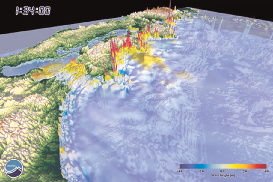
An example of a tsunami simulation (JAGURS code) in the Nankai subduction zone.

2. Hardware

At the time this paper was written, the K computer was the fastest computer in Japan; it was the fastest computer in the world from June 2011 to June 2012. The K computer was manufactured by Fujitsu and named “kei”, the Japanese word for 10 quadrillion (10¹⁶). It is installed at the RIKEN Advanced Institute for Computational Science campus in Kobe, Japan, and is equipped with 82,944 2.0 GHz eight-core SPARC64 VIIIfx processors, based on a distributed memory architecture, for a total of 663,552 cores. It is also equipped with 5184 I/O processors. The K computer uses a proprietary, six-dimensional torus interconnect called Tofu and a Tofu-optimized message-passing interface (MPI) based on an open-source library (e.g. Matsumoto et al., 2012). Users can create applications adapted to one-, two-, or three-dimensional torus networks. A LINPACK performance of 10.51 petaflops has been achieved on the K computer with computing efficiency of 93.2% (Fujitsu Corporation, 2012).

3. Numerical methods

3.1 Tsunami propagation equations

Tsunami simulations are usually conducted in two-dimensional space using nonlinear long-wave equations. These equations can be derived by integrating the Navier–Stokes equations over depth if the horizontal dimension of the simulation is much greater than its vertical dimension. This assumption is valid for tsunamis because the tsunami wavelength associated with large earthquakes is usually much greater than the water depth. If this condition is satisfied, conservation of mass implies that the vertical velocity of the fluid is small. It can be shown from the momentum equation that vertical pressure gradients are nearly hydrostatic and that horizontal pressure gradients are caused by displacement of the pressure surface, the implication being that the horizontal velocity field is constant throughout the depth of the fluid. Vertical integration allows the vertical velocity to be removed from the equations. The equations of motion in nonlinear long-wave theory are expressed as follows (Satake, 1995):

\frac{\partial u}{\partial t} + \frac{u}{R \sin θ} \frac{\partial u}{\partial φ} + \frac{v}{R} \frac{\partial u}{\partial θ} = - \frac{g}{R \sin θ} \frac{\partial h}{\partial φ} - C_{f} \frac{u \sqrt{u^{2} + v^{2}}}{d + h}

(1)

\frac{\partial v}{\partial t} + \frac{u}{R \sin θ} \frac{\partial v}{\partial φ} + \frac{v}{R} \frac{\partial v}{\partial θ} = - \frac{g}{R} \frac{\partial h}{\partial θ} - C_{f} \frac{v \sqrt{u^{2} + v^{2}}}{d + h}

(2)

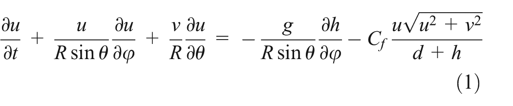
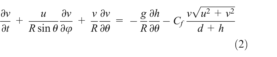
The equation of continuity is

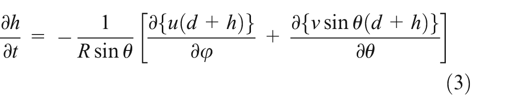
\frac{\partial h}{\partial t} = - \frac{1}{R \sin θ} [\frac{\partial {u (d + h)}}{\partial φ} + \frac{\partial {v \sin θ (d + h)}}{\partial θ}]

(3)

where h is the height of water above the at-rest sea surface, t is time, φ is longitude, θ is colatitude, R is the earth’s radius, u and v are depth-averaged velocities along lines of longitude and latitude, respectively, d is water depth, g is the gravitational constant, and C_f is the nondimensional frictional coefficient.

3.2 Finite-difference scheme

To compute tsunami propagation and areas of inundation using the JAGURS code, Equations (1)–(3) are solved by the finite-difference method using spherical coordinates. To solve these equations, we used the leapfrog, staggered-grid, finite-difference calculation scheme shown in the Appendix. Nonlinear terms in the model are approximated by first-order upwind finite differences and linear terms by two-point centered finite differences. Absorbing boundary conditions are included in the code and optimized to reduce reflections of tsunami waves at the outer boundaries of the simulation. Tsunami inundation on the land is modeled by a moving wet or dry boundary condition, as proposed by Kotani et al. (1998). The computational time step is determined by the Courant–Friendrichs–Lewy condition for a staggered-grid scheme. We used a constant time step for the entire calculation, selecting the minimum time-step value from among those of the nested grids.

The optimized code we developed uses a variable nested algorithm (Figure 2) that allows the spatial resolution of the study region to be easily increased. The ratio of the grid spacing of the parent to child nested grids is 3:1. For communication between the nested grids, the code prepares a correspondence table that contains the set of parent and child grid point indexes for the data to be exchanged. By referring to this index table, data at the edges of the nested child grid are overwritten by linearly interpolated data from its parent nested grid, and the data at the grid points around the boundary of the nested child grid are copied to the corresponding grid points of the nested parent grid at each time step. This two-way intergrid communication achieves seamless propagation of the tsunami between the nested grids.

Figure 2.

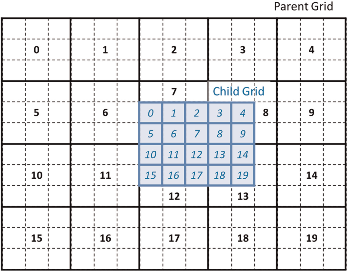
Nesting algorithm and domain decomposition for parallel computation. Numbers indicate message-passing interface ranks assigned for calculation of rectangular subdomains.

3.3 Parallelization

We applied a domain-decomposition method for parallel implementation of the nonlinear long-wave model. We divided the finite-difference grid points of a nested grid into multiple rectangular subdomains, each of the same size, with the number of subdomains equal to the number of MPI processes (Figure 2). An important aspect of decomposing the domain is load balancing. All MPI processes must have equal or almost equal amounts of data to be processed. This condition was achieved by dividing all of the nested grids into the same number of subdomains, and each of these subdomains was associated with one MPI process. For example, computation of the No. 1 subdomain of nested grid A was followed by computation of the No. 1 subdomain of nested grid B, followed in turn by that of nested grid C on the No. 1 computation node. Shared-memory parallel processing with OpenMP was also incorporated into the code to accelerate loop calculations in the subdomains. We also used automatic parallelization of the compiler. The variables h, v, and u in Equations (1)–(3) were exchanged at boundaries between adjoining subdomains by point-to-point communication using the MPI library. A computational flowchart for this code is shown in Figure 3.

Figure 3.

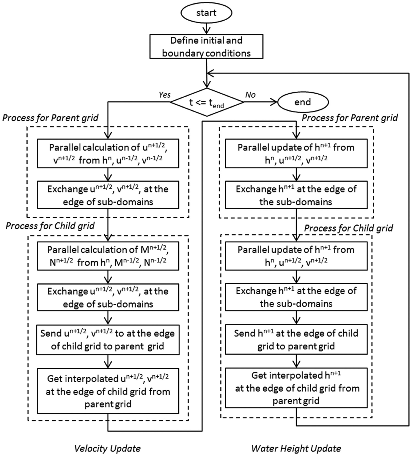
Flowchart of parallel tsunami calculation with the nesting algorithm. This example uses two nested grids, a parent and a child grid, similar to the scheme shown in Figure 2.

The code includes two collective communication methods that allow it to achieve seamless propagation of a tsunami at the boundaries between nested grids in a parallel scheme. The first of these uses MPI_Allreduce (Figure 4(a)), in which each process retains a long communication buffer that can save all of the data to be sent via intergrid communications. The long communication buffers are initialized by zero. Each process copies the assigned parent data needed for intergrid communication to part of the buffer. This is followed by MPI_Allreduce commutation so that each process provides all of the data at the boundary of the nested child grid.

Figure 4.

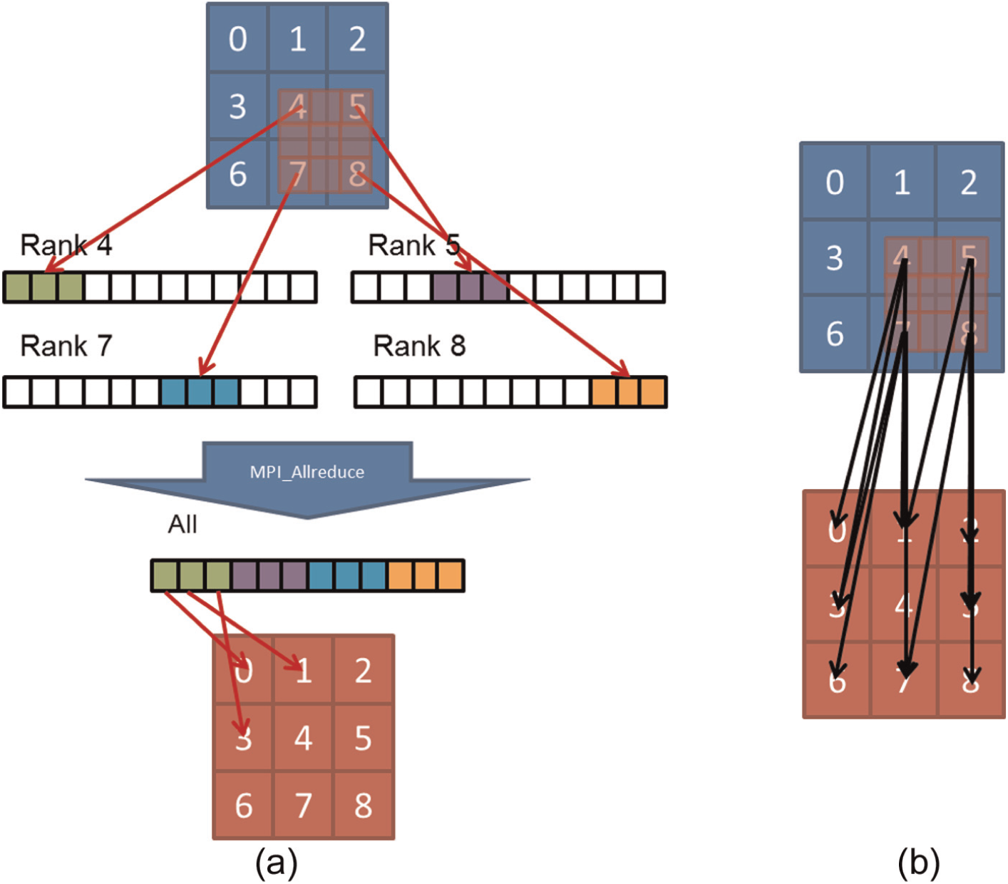
(a) Intergrid communication algorithm using MPI_Allreduce. Blue and red indicate parent and child grids, respectively. Numbers indicate MPI ranks assigned for calculation of the rectangular subdomains. Parent data at the edges of the nested child grid are transferred through the communication buffer to the processes assigned to the nested child grid. (b) Intergrid communication algorithm using MPI_Alltoallv. Parent data at the edges of the child grid are transferred directly to processes assigned to the child grid. (Color online only.)

It is relatively easy to implement the MPI_Allreduce method within the JAGURS code. Moreover, the MPI_Allreduce function on the K computer has been well optimized for Tofu interconnects (Matsumoto et al., 2012). We therefore expected to obtain both easy implementation and high-speed computation. However, in the case of highly parallel execution, there is a disadvantage associated with the use of the long communication buffers. Each process always transfers all of the data in the communication buffer. Thus, the zero-cleared buffers are also transferred multiple times in the network according to the number of parallel processes, which causes a non-negligible increase in the amount of communication in the case of calculations using large numbers of processes.

The second collective communication method uses MPI_Alltoallv for intergrid communication (Figure 4(b)). In contrast to the MPI_Allreduce method, with MPI_Alltoallv each process uses only the minimum length of communication buffer required to contain and transfer the assigned parent data to the nested child grid, thus decreasing the amount of communication required by each process as the number of processes increases. The total amount of communication is therefore constant, regardless of the number of MPI processes. However, the MPI_Alltoallv method has two disadvantages: implementation of this algorithm is complicated, and the MPI_Alltoallv function is not optimized for use in the three-dimensional torus network on the K computer. Here, we attempted to optimize the method for use on the three-dimensional torus network to facilitate large-scale, high-speed tsunami predictions.

4. Analytical models

For our large-scale simulations we selected as our study area the Nankai seismogenic zone off southwestern Japan, where the Philippine Sea tectonic plate is subducting beneath the Eurasia plate at about 4 cm/year. The strain accumulated during subduction has been periodically released by megathrust earthquakes originating in the Nankai trough, some of which have caused great tsunamis. The average recurrence interval of these earthquakes has been estimated to be 100–150 years (Ishibashi and Satake, 1998). After the 2011 Tohoku earthquake, the Cabinet Office of the Japanese government reassessed the risk of great earthquakes and tsunamis in the Nankai trough (Cabinet Office, 2012) and concluded that for a magnitude 9 earthquake and tsunami, a worst-case scenario might involve up to 323,000 fatalities. This severe estimate is based on an earthquake source closer to the coast than that of the 2011 Tohoku earthquake and a tsunami affecting a more heavily populated area than the Tohoku region. We defined two analytical models in the Nankai seismogenic zone (the Nankai and Kochi models) to optimize the JAGURS code. We used the magnitude 9 earthquake model provided by the Cabinet Office in the simulations.

4.1 Nankai model

The Nankai model covered all of southwestern Japan (Figure 5(a)), that is, the area between latitudes 29°–35.9°N and longitudes 130°–141°E (1000 km × 780 km), with a grid spacing of 0.1 arcsec (about 2.5 m). We obtained the bathymetric and topographic data required in the simulation from several sources. The General Bathymetric Chart of the Oceans (British Oceanographic Data Centre, 2010) provides accurate global bathymetry datasets (spatial resolution, 30 arcsec) for the world’s oceans. The M7000 series of digital bathymetric contour maps, a compilation of all locally available bathymetric maps of Japanese coastal waters provided by the Japan Hydrographic Association, is also useful for tsunami simulations. Lidar surveys (remotely sensed laser reflection data) collected along the Japanese coast by the Geospatial Information Authority of Japan provide high-resolution information about the ground surface that is useful for tsunami simulations. These datasets were incorporated and resampled to produce a high-resolution bathymetric grid. In this model, a variable nested algorithm was not used; only one nested grid was defined. The total number of grid points was almost 100 billion. We simulated only the first 20 s of tsunami propagation in a performance test. Then, on the basis of this test we set the time step to 0.005 s, which was sufficient to maintain the stability of the simulation.

Figure 5.

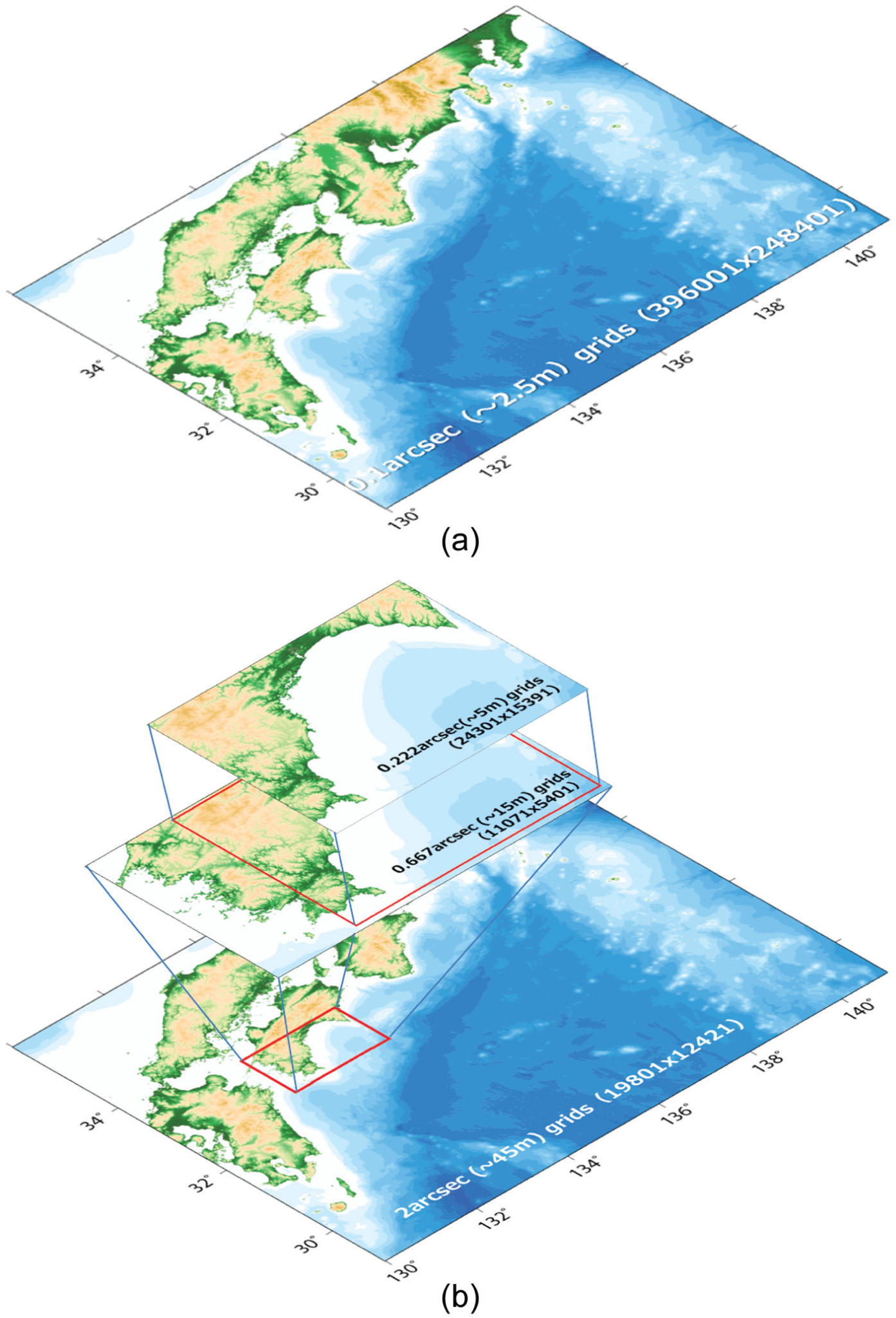
(a) The Nankai model and (b) the Kochi model used in the parallel performance test.

The accuracy of the simulation of the inundation process is not sufficient to investigate the detailed flow dynamics around buildings and other structures because we have not included the three-dimensional shape of buildings and structures in the simulation of this study. The nonlinear long-wave equations cannot solve rapid flows climbing up vertical standing walls or steep slopes. The full three-dimensional Navier–Stokes equations have to be used for detailed simulation of the tsunami flow around buildings. However, the purpose of the present study was to determine how fast we can predict tsunami inundation on land by using high-resolution topographic data for a large area as soon as possible after a great earthquake occurs in order to enhance tsunami evacuation, rescue, and first-aid operations, not to carry out a detailed investigation of the flow dynamics around structures. Two-dimensional nonlinear long-wave models are commonly used to assess maximum flow depth of a tsunami, and such models can be computed much faster than a three-dimensional model. Thus, the accuracy of the two-dimensional, nonlinear, long-wave equations is sufficient, at least for the purpose of this study.

4.2 Kochi model

In Japan, local governments play an important role in emergency operations following earthquakes and tsunamis. They act as intermediaries between affected municipalities and national government agencies, such as the Japan Self-Defense Forces, and they also undertake emergency operations themselves. The Kochi model (Figure 5(b)) was designed to provide a rapid tsunami prediction to a local government such as that of Kochi Prefecture. Kochi Prefecture, which is on Shikoku Island and has a 706-km-long coastline facing the Pacific Ocean, is one of several local government areas where a Nankai trough earthquake and tsunami is predicted to inflict devastating damage. A tsunami height of up to 34 m has been predicted as a worst-case scenario by the Cabinet Office (2012).

For the Kochi model, we used three nested grids (Figure 5(b)). The coarsest grid (2 arcsec spacing) covered the same region as the grid used for the Nankai model. In other words, the Kochi model can be treated as a nested Nankai model. The finest nested grid covered Kochi Prefecture with a grid spacing of 2/9 arcsec (about 5 m). The finest nested grid included a sea region in which the bathymetric data resolution was much lower than the grid spacing. We therefore interpolated the bathymetric data to fit the grid spacing. Because all nested grids in the calculation scheme must be rectangular, it was necessary to grid a part of the coastal sea region adjacent to the land region at high resolution. An intermediate nested grid (2/3 arcsec) was used to link the coarsest and finest nested grids, because the grid spacing ratio of the parent to child nested grids must be 3:1. Tsunami propagation in the shaded region of the coarse grid (i.e. the part covered by the fine grid) was also computed and then discarded. In terms of the total elapsed time, it is not important whether or not calculations for the shaded zone are processed. In any case, calculations for the shaded zone cannot proceed to the next step until those for the zone not overlapping the fine grid are finished. The total number of grid points was 0.68 billion. We simulated the first 5 h of a tsunami generated by a magnitude 9 Nankai trough earthquake with a time step of 0.015 s. This time period ensured that the simulation would include the maximum tsunami height reached in Kochi Prefecture.

5. Performance for the velocity update loop

Our measurements of subroutine runtimes in the original JAGURS code identified the velocity update loop as the most time-consuming process, accounting for more than 70% of the total time of the main loop. The process contained many IF statements that caused long waiting periods for floating-point instructions to be completed (53% of the elapsed time used in the velocity update loop). Neither SIMD (single instruction multiple data) optimization nor software pipelining was performed by the compiler. We therefore introduced the following code enhancements (Figure 6).

In the original code, propagating waves of dry grid cells (i.e. on land, where there was no propagating wave) were not processed in the velocity update loop. However, we modified the code to apply the propagating wave processing to all grid cells regardless of whether they were dry or wet. This allowed SIMD optimization and software pipelining.

In grid cells located on land, velocities were overwritten with zeros after the first pass through the velocity update loop. Because of the complicated IF statement structure, SIMD optimization and software pipelining were not applied during this overwrite, but the time cost of this operation was negligible.

To further improve SIMD optimization and software pipelining of propagating wave processing, we divided the inner loop into several subloops, each with only one IF statement. We also used an option that enabled the compiler to generate masked instructions.

Figure 6.

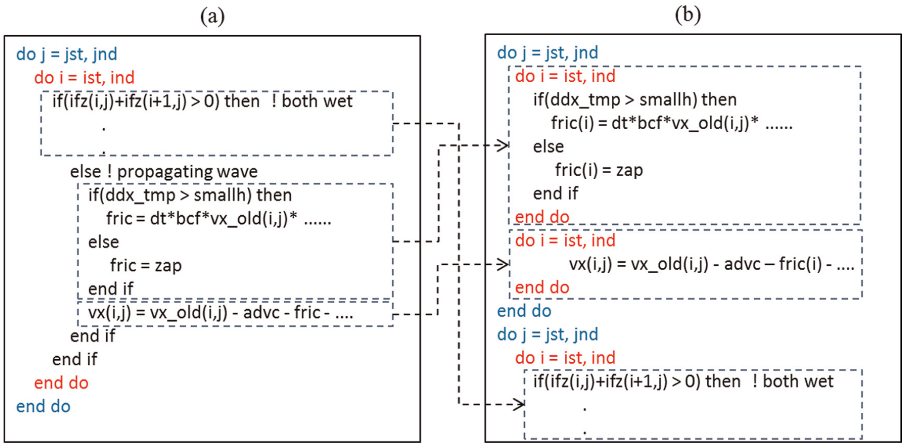
Simulation code (a) before and (b) after optimization of the velocity update loop.

For further optimization, we attempted to use a cell-blocking method to remove dry grid cells on land from the computation. However, JAGURS uses a wet/dry boundary condition (Kotani et al., 1998) to express tsunami inundation on land. Grid cells in the coastal region may be dry at one time, but wet another time. Thus, to remove dry cells from the computation for enhanced SIMD optimization, the program has to check whether or not a block divided by cell blocking includes dry cells at every time step before the velocity update calculation. Because this procedure results in a long overhead time, this optimization was unsuccessful.

Our arithmetic optimization successfully enhanced SIMD optimization and software pipelining in the velocity update loop (Table 1). The waiting time for floating-point instructions to be completed was reduced by a factor of 11, and the elapsed time by a factor of 2. Performance efficiency for the entire velocity update loop on 16 nodes of the K computer was increased from 7.34% to 17.89%.

Table 1.

Results of optimization of the velocity update loop.

	Original	Optimized
Elapsed time [s]	45.72	22.89
Wait for floating-point instruction [s]	24.23	2.16
Percentage of SIMD instructions	0.00	29.51
Relative speed increase	1.00	2.00
Efficiency [%]	7.34	17.89

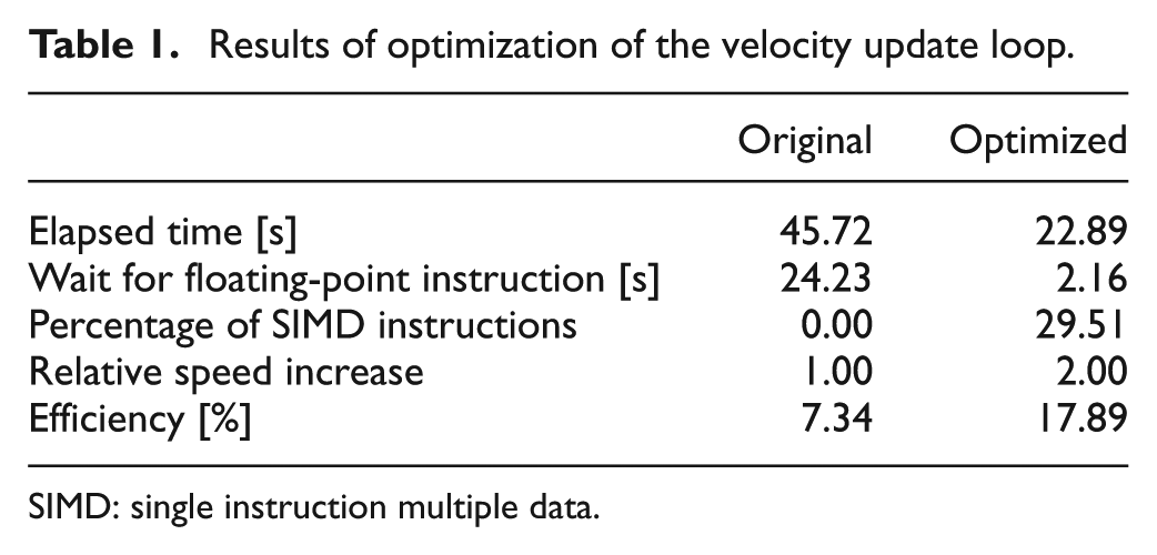
SIMD: single instruction multiple data.

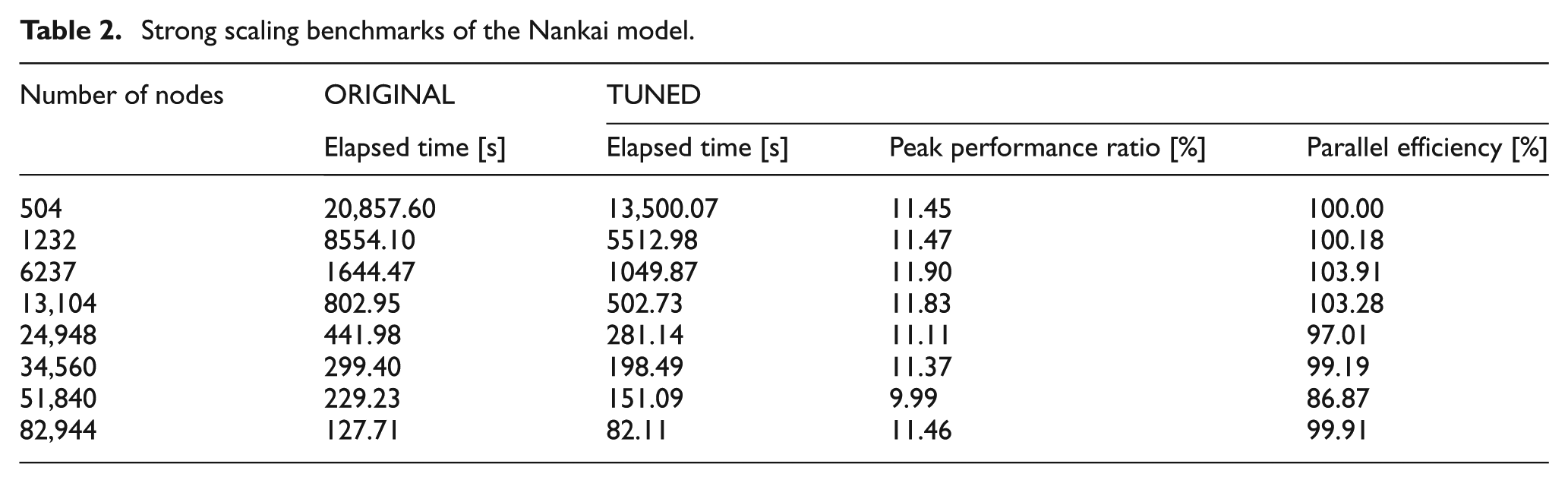
We applied the optimized code to the Nankai model described in section 4.1. We conducted a strong scaling test for node usage from 504 nodes up to the full system capability of 82,944 nodes. Total memory usage for the full system calculation was about 27 TB. The performance test indicated excellent scaling and showed that performance was maintained at a high level up to full system operation (Figure 7). A maximum processing speed of 1.2 petaflops was attained, corresponding to 11.5% of the peak speed on 82,944 nodes of the K computer (Table 2). A 20-s simulation of the large-scale and high-resolution Nanai model with the K’s 82,844 nodes took 82.11 s. In the single-layered Nankai model, only point-to-point communication was needed to exchange data at the boundaries between adjoining subdomains. Collective communications were not employed, so the time cost of communication did not increase with the number of processes, thus providing good scaling performance.

Figure 7.

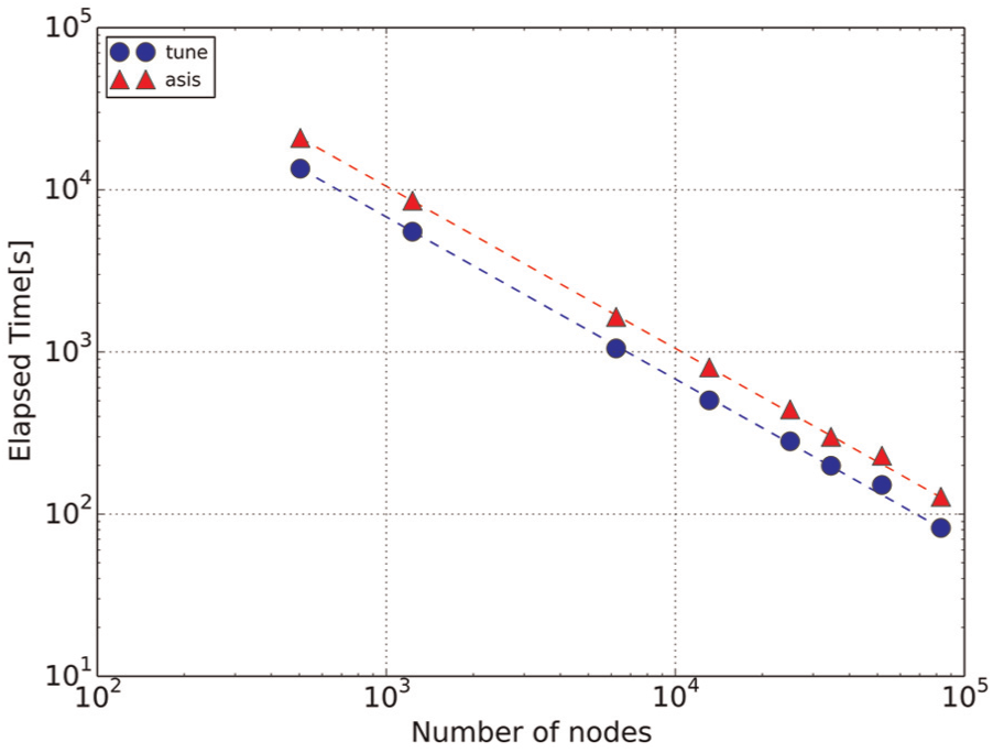
Elapsed time required for calculation of the Nankai model. Data obtained with the original code are shown by red triangles, and data obtained with the tuned code after optimization of the velocity update loop are shown by blue circles. The dashed lines indicate ideal performance. (Color online only.)

Table 2.

Strong scaling benchmarks of the Nankai model.

Number of nodes	ORIGINAL	TUNED
Number of nodes	Elapsed time [s]	Elapsed time [s]	Peak performance ratio [%]	Parallel efficiency [%]
504	20,857.60	13,500.07	11.45	100.00
1232	8554.10	5512.98	11.47	100.18
6237	1644.47	1049.87	11.90	103.91
13,104	802.95	502.73	11.83	103.28
24,948	441.98	281.14	11.11	97.01
34,560	299.40	198.49	11.37	99.19
51,840	229.23	151.09	9.99	86.87
82,944	127.71	82.11	11.46	99.91

We also performed a strong scaling test of the Kochi model described in section 4.2 and compared the performances of the MPI_Allreduce and MPI_Alltoallv collective communication methods (Figure 8 and Table 3). For 8748 nodes, the performance of the MPI_Allreduce method, which includes unnecessary intergrid communications, was about 10 times better than that of the MPI_Alltoallv method (Table 3). This indicates that the MPI_Allreduce function, originally optimized for the three-dimensional torus network on the K computer, efficiently overcame the unnecessary communications between nested grids. In contrast, the MPI_Alltoallv function was not optimized for the torus network, which accounts for its inferior performance, even though this method eliminates unnecessary intergrid communications. Furthermore, data communications between nested grids occurred only along the nested boundaries, so relatively small amounts of data were sent by collective communication. This is another reason for the superior performance of the MPI_Allreduce method.

Figure 8.

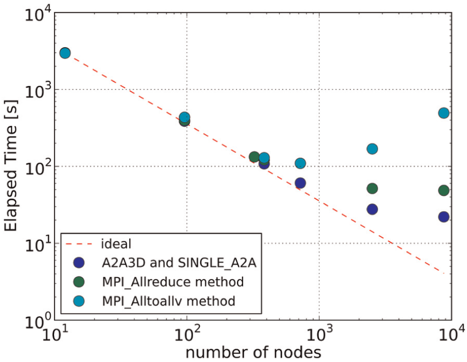
Strong scaling test of the Kochi model. Results obtained using the MPI_Allreduce method (green), the MPI_Alltoallv method (cyan), and the A2A3D and SINGLE_A2A (optimized MPI_Alltoallv) method (blue) are shown. See section 6 in the text for a discussion of A2A3D and SINGLE_A2A. (Color online only.)

Table 3.

Strong scaling benchmarks of the Kochi model.

Number of nodes	Elapsed time [s]
Number of nodes	MPI_Alltoallv method	MPI_Allreduce method	A2A3D and SINGLE_A2A^a
12	2966.90	2997.18	2965.01
96	435.29	396.30	386.20
324	N/A	132.61	N/A
384	129.28	121.50	108.08
720	109.43	N/A	60.79
2520	168.58	51.42	27.66
8748	493.28	48.57	22.03

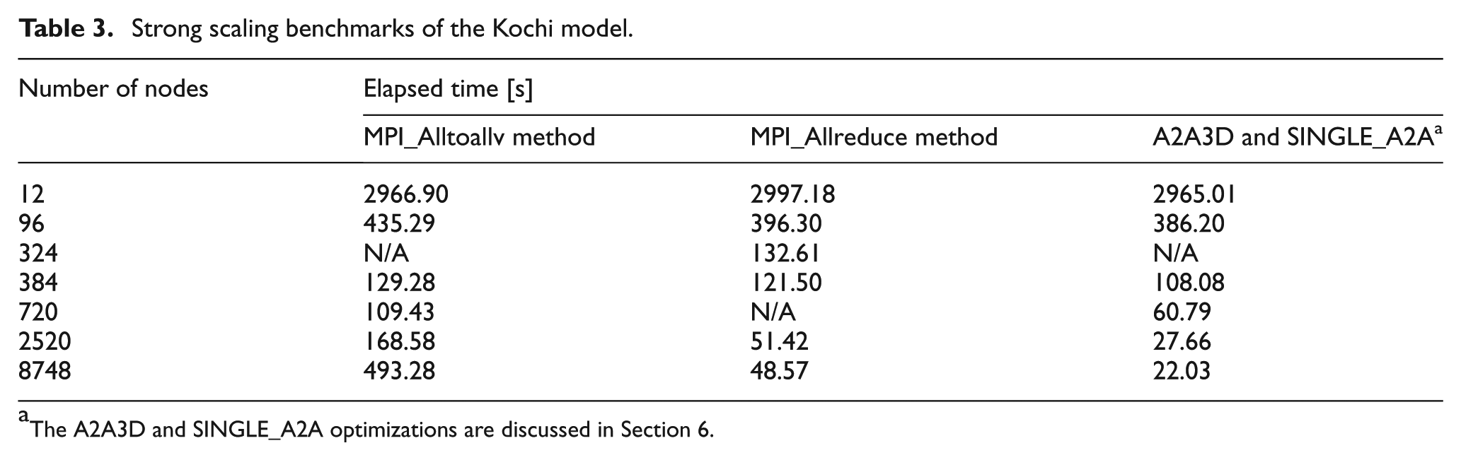
The A2A3D and SINGLE_A2A optimizations are discussed in Section 6.

However, the increase in processing speed with the MPI_Allreduce method tailed off for higher numbers of nodes (Figure 8). Comparison of the elapsed time for velocity and wave update calculations with those for intergrid communication processes (Figure 9) showed that intergrid communication accounted for 72% of the elapsed time. Thus, although the optimization of the velocity loop improved the performance of the Kochi calculation, it was not apparent with a large number of nodes because intergrid communications tasks were dominant. Therefore, to further improve processing time, it was necessary to optimize intergrid communications on the K computer.

Figure 9.

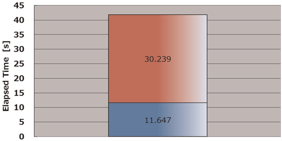
Comparison of elapsed time required for calculations (velocity and wave height update routine) and intergrid communications for 5184 nodes and 4001 steps in the Kochi model. Velocity update routine and intergrid communications are shown in blue and red, respectively. (Color online only.)

6. Parallel optimization

6.1 Optimization of intergrid communication

We optimized the MPI_Alltoallv collective communication method for the three-dimensional torus network to increase performance. In the original MPI_Alltoallv method (Figure 10(a)), each process requires n– 1 communications for parallel implementation of n processes, where the frequency of communication of each process is O(n). In the optimized MPI_Alltoallv method (Figure 10(b)), the communication was divided into three directions along the x, y, and z axes corresponding to the three-dimensional torus network. By assuming n = n_x × n_y × n_z, the frequency of communication of each process was dramatically decreased from O(n) to O(n_x) + O(n_y) + O(n_z). This algorithm provides a further advantage in that it reduces network congestion. We named this new optimization method A2A3D.

Figure 10.

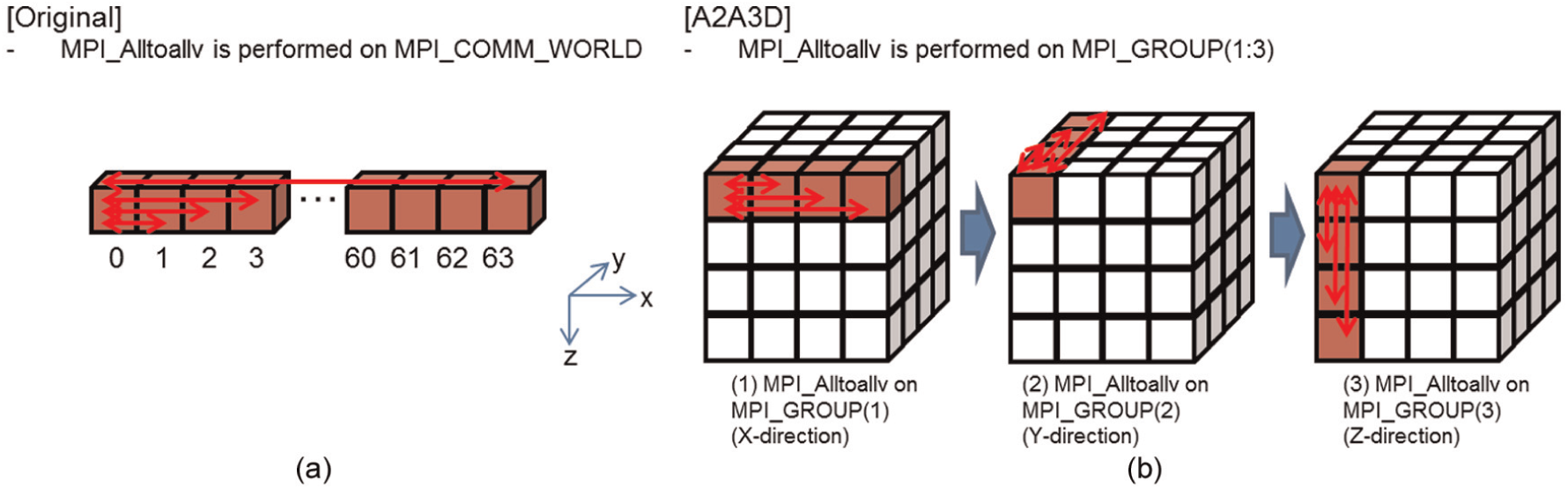
Schematic examples of 64 processes of (a) the original MPI_Alltoallv algorithm and (b) the A2A3D algorithm developed for the three-dimensional torus network of Tofu interconnect on the K computer, implemented with the MPI_Alltoallv routine.

It should be noted that two-directional process mapping is more effective than three-directional mapping in the case of single nested grid calculations, as in the Nankai model, because the nonlinear long-wave equations are written in two dimensions. However, for tsunami calculations with multiple nested grids, as in the Kochi model, the collective communications that are needed to implement the intergrid communication are more efficient with three-directional process mapping.

In addition to the implementation of A2A3D, where possible we combined multiple A2A3D communications into a single communication to more effectively use network bandwidth and to reduce unnecessary overhead caused by multiple calling of the MPI_Alltoallv function. We named this optimization SINGLE_A2A.

6.2 Performance results for intergrid communication

The A2A3D and SINGLE_A2A optimizations increased the speed of intergrid communication by a factor of about three. The elapsed time for intergrid communications was comparable to that for computation of velocity and wave height. Together, these optimizations increased total performance by a factor of 1.92 (Figure 11). Scalability was also improved (Figure 8). Peak performance was achieved by using the optimized MPI_Alltoallv algorithm on 8748 nodes of the K computer to solve the Kochi model, where the peak performance rate was 2.58%. The elapsed time was shortened by a factor of 22.4 compared with the original MPI_Alltoallv method and by a factor of 2.2 compared with the MPI_Allreduce method (Table 3).

Figure 11.

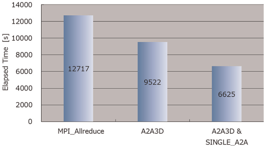
Comparison of the elapsed time obtained with the original MPI_Allreduce algorithm with those obtained after the implementation of the A2A3D and the A2A3D and SINGLE_A2A optimizations.

7. Discussion and conclusions

We developed tsunami simulation code to provide large-scale tsunami predictions. For performance measurements, we constructed the Nankai model, an extremely large single-grid model (100 billion grid points with 2.5-m spacing) covering southwestern Japan. A great Nankai earthquake would devastate the entire coastal region of southwestern Japan. Grid points with a spacing of 2.5 m are required for tsunami inundation modeling in urban areas, where the three-dimensional shapes of buildings and breakwaters are embedded in the topography. This is why we decided to investigate a large-scale, high-resolution model in this study. The performance of simulations on the K computer was considerably enhanced by SIMD optimization and software pipelining. A simulation using the Nankai model achieved an average processing speed of 1.2 petaflops, corresponding to 11.5% of the full-system peak speed of the K computer. This Nankai model could be solved within an elapsed time four times as long as real time. Although the Nankai model is not capable of real-time tsunami prediction, it is useful for applications such as the construction of a pre-computing database of tens of thousands of tsunami scenarios.

The Kochi model that we used consists of 0.68 billion grid cells, and the area with the finest grid (180 km × 120 km) was resolved with a grid spacing of about 5 m. For the Kochi calculations, we enhanced the use of the three-dimensional torus network. With this model, a large-scale tsunami simulation for hazard assessment was completed in about 30% of real time. Codes similar to ours that solve nonlinear long-wave equations using nested algorithms have been reported (e.g. Imamura, 1996; Titov and González, 1997; Liu et al., 1998), but because they do not include MPI parallelization techniques, they cannot be used for large-scale simulations such as our Kochi simulation. The only comparable simulation incorporating MPI parallelization techniques is that of Oishi et al. (2013), who solved nonlinear, long-wave equations by applying the finite volume method to unstructured cells on 16,384 nodes of the K computer to obtain a tsunami prediction in less than real time with a computation model of about 16.8 million cells. Two 5 km × 7 km areas were resolved with a 5-m mesh spacing in their study.

It took 3.5 h to obtain a 5-h simulation with the Kochi model without implementation of the A2A3D and SINGLE_A2A optimizations, but less than 1.5 h with them. During the first 1.5 h of the 2011 Tohoku tsunami disaster, only patchy information was available, and the overall gravity of the situation was unclear. The computational speed of the code we have developed will allow high-resolution tsunami simulations to be completed over broad regions much earlier than has been possible heretofore, so that meaningful tsunami predictions can be made that will greatly accelerate the planning and execution of effective emergency rescue and relief operations during future tsunami disasters.

Further studies aimed at high-speed, high-spatial-resolution, and broad-scale for tsunami disaster mitigation should be carried out. We would be able to remove dry cells from the computation. By taking cell blocking with a proper size, SIMD optimization becomes more effective to shorten the computational time. It may be possible to achieve a performance of the Kochi model (now at 2.58% of peak speed) comparable to that with the Nankai model (11.5% of peak speed) by introducing an overlap between computation and communication to hide the communication time. At the beginning of this study, the intergrid communication took much longer than the calculation. Our optimizations eventually reduced it to a time period comparable to that used for the flow calculations. It is now at a stage where the possibility of overlapping computation and communication to further improve the model performance should be investigated. We plan to investigate this possibility in a future paper so that we can contribute to the mitigation of the effects of future major disasters comparable to the 2011 Tohoku, 2010 Chile, and 2004 Sumatra tsunamis.

Footnotes

Appendix: finite-difference scheme for nonlinear,long-wave equations

The finite-difference calculation is performed in a staggered-grid system (Figure A1). Because time integration is solved by a leapfrog method, the water height (h) is defined at time $t = n Δ t$ , and the depth-averaged velocities (u, v) are defined at $t = (n - 1 / 2) Δ t$ , where $Δ t$ is the time step and $n = 1, 2, 3 \dots$ . Equation (1) can be written in finite-difference form as

(A1)

\begin{matrix} u^{n + \frac{1}{2}} = u^{n - \frac{1}{2}} - \frac{u_{i, j}^{n - \frac{1}{2}}}{R \sin θ} \frac{Δ t}{Δ φ} (u_{i + 1, j}^{n - \frac{1}{2}} - u_{i, j}^{n - \frac{1}{2}}) \\ - \frac{{\bar{v}}_{i, j}^{n - \frac{1}{2}}}{R} \frac{Δ t}{Δ θ} (u_{i, j + 1}^{n - \frac{1}{2}} - u_{i, j}^{n - \frac{1}{2}}) \\ + \frac{g}{R \sin θ} \frac{Δ t}{Δ φ} (h_{i + 1, j}^{n} - h_{i, j}^{n}) - C_{f} \frac{u_{i, j}^{n - \frac{1}{2}} \sqrt{u_{i, j}^{n - {\frac{1}{2}}^{2}} + {\bar{v}}_{i, j}^{n - {\frac{1}{2}}^{2}}}}{d_{u (i, j)} + h_{u (i, j)}} Δ t \end{matrix}

where, because of the staggered-grid system (Figure A1),

(A2)

{\bar{v}}_{ij} = \frac{v_{i, j} + v_{i + 1, j} + v_{i, j - 1} + v_{i + 1, j - 1}}{4}

(A3)

d_{u (i, j)} + h_{u (i, j)} = \frac{d_{ij} + d_{i + 1, j} + h_{i, j} + h_{i + 1, j}}{2}

Note that the second and third terms on the right-hand side of equation (A1) are approximated by upwind finite differences.

Similarly, Equation (2) can be written in finite-difference form as

(A4)

\begin{matrix} v^{n + \frac{1}{2}} & = v^{n - \frac{1}{2}} - \frac{{\bar{u}}_{i, j}^{n - \frac{1}{2}}}{R \sin θ} \frac{Δ t}{Δ φ} (v_{i + 1, j}^{n - \frac{1}{2}} - v_{i, j}^{n - \frac{1}{2}}) \\ - \frac{{\bar{v}}_{i, j}^{n - \frac{1}{2}}}{R} \frac{Δ t}{Δ θ} (v_{i, j + 1}^{n - \frac{1}{2}} - v_{i, j}^{n - \frac{1}{2}}) + \frac{g}{R} \frac{Δ t}{Δ φ} (h_{i, j + 1}^{n} - h_{i, j}^{n}) \\ - C_{f} \frac{v_{i, j}^{n - \frac{1}{2}} \sqrt{{\bar{u}}_{i, j}^{n - {\frac{1}{2}}^{2}} + {\bar{v}}_{i, j}^{n - {\frac{1}{2}}^{2}}}}{d_{v (i, j)} + h_{v (i, j)}} Δ t \end{matrix}

where, because of the staggered-grid system (Figure A1),

(A5)

{\bar{u}}_{i, j} = \frac{u_{i, j} + u_{i + 1, j} + u_{i - 1, j + 1} + u_{i, j + 1}}{4}

(A6)

d_{v (i, j)} + h_{v (i, j)} = \frac{d_{i, j} + d_{i, j + 1} + h_{i, j} + h_{i, j + 1}}{2}

The second and third terms on the right-hand side of Equation (A4) are also approximated by upwind finite differences.

Equation (3) can be written in finite-difference form as

(A7)

\begin{matrix} h^{n + 1} \\ = h^{n} \\ - \frac{Δ t}{R \sin θ} [(\frac{u_{i, j}^{n + \frac{1}{2}} (d_{u (i, j)} + h_{u (i, j)}) - u_{i - 1, j}^{n + \frac{1}{2}} (d_{u (i - 1, j)} + h_{u (i - 1, j)})}{Δ φ} \\ + \frac{v_{i, j}^{n + \frac{1}{2}} \sin (θ) (d_{v (i, j)} + h_{v (i, j)}) - v_{i, j - 1}^{n + \frac{1}{2}} \sin (θ - Δ θ) (d_{v (i, j - 1)} + h_{v (i, j - 1)})}{Δ θ})] \end{matrix}

At time $t = n Δ t$ , we calculate $u^{n + \frac{1}{2}}$ and $v^{n + \frac{1}{2}}$ by substituting $h^{n}$ , $v^{n - \frac{1}{2}}$ , and $u^{n - \frac{1}{2}}$ into Equations (A1) and (A4), and we substitute the calculated $u^{n + \frac{1}{2}}$ and $v^{n + \frac{1}{2}}$ values into Equation (A7) to obtain $h^{n + 1}$ . Then $h^{n + 1}$ , $u^{n + \frac{1}{2}}$ , and $v^{n + \frac{1}{2}}$ are used for solving equations (A1), (A4), and (A7) in the next time step.

Acknowledgements

We thank anonymous reviewers for constructive comments. Computational resources of the K computer were provided by the RIKEN Advanced Institute for Computational Science through the High Performance Computing Infrastructure System Research project (Project ID: hp130014).

Declaration of Conflicting Interests

The author(s) declared no potential conflicts of interest with respect to the research, authorship, and/or publication of this article.

Funding

The author(s) disclosed receipt of the following financial support for the research, authorship, and/or publication of this article: This study was partially funded by the Strategic Programs for Innovative Research: Advanced Prediction Researches for Natural Disaster Prevention and Reduction (Field 3) initiative of the Japan Agency for Marine-Earth Science and Technology.

Author biographies

Toshitaka Baba’s research career began in 1999 when he joined the JAMSTEC as a junior research assistant. The work involved helping research scientists do numerical modeling to study subduction zone dynamics, including the study of earthquakes and tsunamis. After receiving his PhD from Kanazawa University, his role at JAMSTEC changed to a full-time research position. The research continued to focus on subduction zone earthquakes and tsunamis, but he also began work on using high-performance computers to study these. He has been a professor at the University of Tokushima since January 2015.

Kazuto Ando works in the Center for Earth Information Science and Technology, JAMSTEC. He supports research activities in Strategic Programs for Innovative Research: Advanced Prediction Researches for Natural Disaster Prevention and Reduction (Field 3).

Daisuke Matsuoka received his BE, ME and PhD degrees from Ehime University, Japan, in 2003, 2005 and 2008, respectively. He has been working as a research scientist at JAMSTEC since 2009. He has also been a visiting associate professor at the Tokyo Institute of Technology since 2015. His research interests include scientific visualization, virtual reality, and numerical simulation.

Mamoru Hyodo is a researcher in the Earthquake and Tsunami Forecasting System Research Group, Research and Development (R&D) Center for Earthquake and Tsunami, JAMSTEC. He simulate generations of the great subduction zone earthquakes on high-performance computers.

Takane Hori leads the Earthquake and Tsunami Forecasting System Research Group, R&D Center for Earthquake and Tsunami, JAMSTEC.

Narumi Takahashi is the vice-director, R&D Center for Earthquake and Tsunami, JAMSTEC. His research major is in the crustal structure in the subduction zones. He and his team are also developing a tsunami prediction system using high-performance computers.

Ryoko Obayashi is a modeling specialist of tsunamis in the Earthquake and Tsunami Monitoring Research Group, R&D Center for Earthquake and Tsunami, JAMSTEC.

Yoshiyuki Imato is a technical staff member in the Center for Earth Information Science and Technology, JAMSTEC. He is a specialist in computing hardware.

Dai Kitamura is a technical staff member in the Center for Earth Information Science and Technology, JAMSTEC.

Hitoshi Uehara has received his Ph.D. at Ibaraki University in 2000. He joined the Earth Simulator Research and Development Center in Japan Atomic Energy Institute, as a Post Doctor. After the completion of the Earth Simulator in 2002, he has taken a full-time research position at Earth Simulator Center in the Japan Agency for Marine-Earth Science and Technology (JAMSTEC). He has been working about program tuning, scientific visualization and promotion of industrial use on JAMSTEC supercomputers. He has been the Group Leader of technical support team for JAMSTEC supercomputer users since 2009.

Toshihiro Kato belongs to the 1st Government and Public Solution Division, NEC Corporation. He is in charge of performance optimization and development for high-performance computing applications.

Ryotaro Saka received his BS degree in information engineering from Yamagata University in 1999. He joined NEC Informatec Systems Ltd in 2000 and is now an Assistant Manager of the Advanced Technology Solutions Division of NEC Informatec Systems.

References

Baba

Takahashi

Kaneda

. (2014) Tsunami inundation modeling of the 2011 Tohoku earthquake using three-dimensional building data for Sendai, Miyagi Prefecture, Japan. In: Fandiño

. (eds) Tsunami Events and Lessons Learned, Advances in Natural and Technological Hazards Research. Vol. 3 35. Dordrecht: Springer, pp.89–98.

British Oceanographic Data Centre (2010) GEBCO (General Bathymetric Chart of the Oceans). Available at: http://www.gebco.net/data_and_products/gridded_bathymetry_data (accessed 1 July 2014).

Burbidge

Cummins

Mleczko

. (2008) A probabilistic tsunami hazard assessment for Western Australia. Pure Applied Geophysics 165 (11–12): 2059–2088.

Cabinet Office (2012) Government of Japan, Nankai trough earthquake damage estimation. Available at: http://www.bousai.go.jp/jishin/nankai/nankaitrough_info.html (in Japanese) (accessed 1 July 2014).

Fujitsu Corporation (2012) “K computer” achieves goal of 10 petaflops. Available at: http://www.fujitsu.com/global/news/pr/archives/month/2011/20111102-02.html (accessed 1 July 2014).

Imamura

(1996) Simulation of wave-packet propagation along sloping beach by TUNAMI-code. In: Yeh

. (eds) Long-Wave Runup Models. Singapore: World Scientific, pp.231–241.

Imamura

Koshimura

Ooya

. (2011) Tsunami simulation for the 2011 off the Pacific coast of Tohoku Earthquake: Tohoku university model version 1.0 (in Japanese). Available at: http://www.tsunami.civil.tohoku.ac.jp/hokusai3/J/events/tohoku_2011/model/11061vers1.0.pdf (accessed 1 July 2014).

Ishibashi

Satake

(1998) Problems on forecasting great earthquakes in the subduction zones around Japan by means of paleoseismology (in Japanese). Journal of the Seismological Society of Japan Zisin 50: 1–21.

Jakeman

Nielsen

VanPutten

. (2010) Towards spatially distributed quantitative assessment of tsunami inundation models. Ocean Dynamics. 60(5): 1115–1138.

10.

Kamigaichi

(2009) Tsunami forecasting and warning. In: Meyers

(ed.) Encyclopedia of Complexity and Systems Science. New York: Springer, pp. 9592–9618.

11.

Kawaguchi

Kaneda

Araki

. (2012) Reinforcement of seafloor surveillance infrastructure for earthquake and tsunami monitoring in western Japan. In: OCEANS’12 MTS/IEEE, Yeosu.

12.

Kotani

Imamura

Shuto

(1998) Tsunami inundation calculation and damage estimation method using GIS. Proceedings of Coastal Engineering JSCE 45: 356–360.

13.

Liu

PLF

Woo

Cho

(1998) Computer programs for tsunami propagation and inundation. Technical Memorandum of Cornell University, p.104.

14.

Matsumoto

Adachi

Sumimoto

. (2012) Implementation and evaluation of MPI_Allreduce on the K Computer (in Japanese). IPSJ Transactions on Advanced Computing Systems (ACS) 5: 152–162.

15.

Monastersky

(2012) The next wave: What can scientists learn from the Tohoku tragedy to improve tsunami forecasting and save lives? Nature 483: 144–146.

16.

National Police Agency (2014) Damage caused by the 2011 off the Tohoku Pacific coast earthquake (in Japanese). Available at: http://www.npa.go.jp/archive/keibi/biki/higaijokyo.pdf (accessed 1 July 2014).

17.

Oishi

Roberts

Imamura

. (2013) Tsunami inundation simulations on a supercomputer. In: ITS2013 abstract book, p.82.

18.

Satake

(1995) Linear and Nonlinear Computations of the 1992 Nicaragua Earthquake Tsunami. Pure and Applied Geophysics 144(3–4): 455–470.

19.

Thio

Somerville

Inchinose

(2008) Probabilistic analysis of tsunami hazards in Southeast Asia. Journal of Earthquake and Tsunami 1(2): 119–137.

20.

Titov

González

(1997) Implementation and testing of the Method of Splitting Tsunami (MOST) model. Technical Memorandum ERL PMEL–112, Government Printing Office, Seattle, WA, p.11.