
Abstract
Compared with a hash table, a Bloom filter (BF) is more space efficient for supporting fast matching through a controllable and acceptable false positive probability. The space size of the basic BF is predetermined based on the expected number of elements to be stored. However, we cannot predict the space scale of a BF for dynamic sets. It is still challenging for the two existing solutions, scalable BF (SBF) and dynamic BF (DBF), to manipulate dynamic data sets with low memory overhead but achieving high performance. This article presents a partitioned BF (Par-BF) for dynamic data sets. Compared with DBF and SBF, Par-BF is able to leverage a sweet spot between high performance and low overhead by a group of formulas to support fast concurrent matching. Specifically, the size and the range of the false positive probability in Par-BF can be deliberately derived. From our trace-driven experimental results, the input/output operations per second of Par-BF outperforms that of DBF and SBF by 10× to 14× and by 3× to 8×, respectively. Besides, through our proposed garbage collection policy, Par-BF consumes less than half of the memory usage of SBF.
1. Introduction
We are now living in an era awash in data, and the amount of digital data in data centers is expected to double annually from today to 2020 (Gantz and Reinsel, 2012). High-performance data-intensive processing is in an irreversible high demand trend (e.g. scientific computing). Specially, target objects from large-scale and complex data sets always have to be retrieved before further processing.
Indexing techniques have been widely used to accelerate object query time using a certain amount of fast memory space. Building a highly effective index for data-intensive distributed computing has been widely studied (e.g. Hadoop). Through using an appropriate indexing technique, we can quickly detect the repetitive objects and thus reduce remote input/outout (I/O) transfer time and eventually speedup the object retrieval process. Hadoop++ (Dittrich et al., 2010) is an improved Hadoop framework to provide a noninvasive, DBMS-independent indexing function, coined Trojan Index, to accelerate the query runtime of HadoopDB (Abouzeid et al., 2009). Sailfish (Rao et al., 2012) improves disk I/O performance in Hadoop via building an index in the Map/Reduce layer to optimally sort and aggregate the intermediate data.
A critical challenge in designing an effective index is how we can reduce space overhead as much as possible while guaranteeing indexing throughput. Compared with a hashing-based index, a Bloom filter (BF) is more spaceefficient for set membership query in terms of is element x in set S? at the cost of a false positive probability (fpp) (Bloom, 1970). Nonetheless, the space saving often outweighs this drawback when fpp is in an acceptable range. An index entry in a standard BF only consumes about
One of the key problems of BFs is false positive. False positive denotes that an item actually does not belong to the set, but the BF falsely reports it is in. On one hand, when the false positive occurs, an extra round trip I/O in the much slower backup indexing is issued to validate the result, leading to indexing throughput degrading sharply. On the other hand, more memory is consumed when the expected fpp is set to a smaller one. Therefore, fpp is expected in an acceptable range to balance the trade-off of indexing throughput and memory overhead (Almeida et al., 2007).
In order to keep the actual false positive rate under the expected fpp, the maximum number of elements to be indexed in a standard BF is usually predetermined as n. However, we cannot precisely predict the scale of elements in dynamic data sets. This leads to the challenge to get a list of flexible sub-BFs. Scalable BF (SBF) (Almeida et al., 2007) and dynamic BF (DBF) (Guo et al., 2010) are two typical design to address this issue. Both DBF and SBF are made up of a series of one or multiple sub-BFs. When the current sub-BF gets full (up to n elements), a new one is added into the list to serve new element insertions. Typically, the space of each sub-BFs is much less than the overall pre-allocated shared memory space. However, SBF and DBF lack further optimization to accommodate with the trade-off between indexing performance and memory cost. The main problem of DBF is not able to control the overall fpp, while SBF does not support BF-based algebra operations for simplifying resource management (e.g. bloomjoin).
This article presents parallel partitioned BF (Par-BF) to support fast element membership query for large dynamic sets. Par-BF partitions the whole required memory space into disjointed sub-BF lists. Each sub-BF list can hold maximal N elements. Each sub-BF list can contain se homogeneous sub-BFs at most. A thread is assigned into each sub-BF list to do matching. An effective way for assigning thread number is making it equal to the number of CPU cores (Pusukuri et al., 2011). There are two major objectives of designing Par-BF. The first one is compulsorily supporting useful bit vector-based algebra operations. The other one is compulsorily controlling the fpp in each matching thread. Even though DBF and SBF can be extended to multi-thread environment, to meet the heterogeneous performance/cost demand, some essential parameters of Par-BF should be well derived as follows.
How can we choose proper fpp values? We need to determine the following two values to control the overall fpp. One is the expected upper bound value of fpp in each sub-BF list, Fmax. The other is the expected fpp of each sub-BF, fppe.
How can we tune the memory space of Par-BF to balance the performance requirement and memory consumption?
In Table 1, we summarize the improvement of Par-BF, compared with DBF and SBF. From our trace-driven evaluated results, the input/output operations per second (IOPS) of Par-BF outperforms that of DBF and SBF, by 10× to 14× and 3× to 8×, respectively. Besides, through our garbage collection policy, the memory overhead of Par-BF is less than half of SBF.
Comparison results of SBF, DBF, and Par-BF.
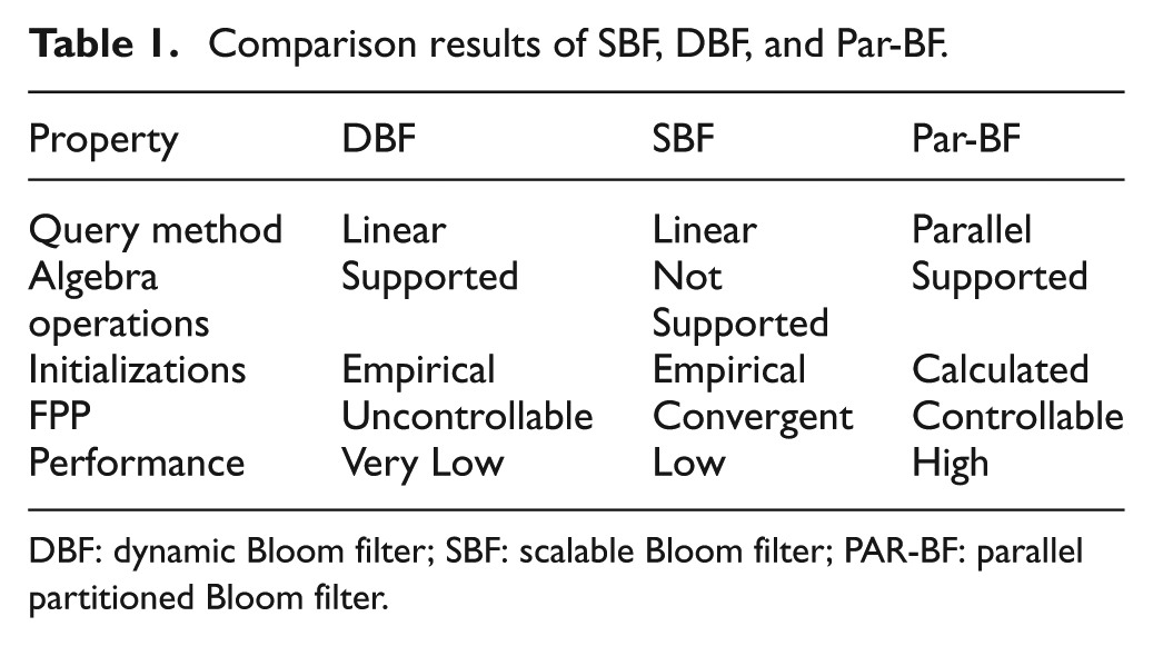
DBF: dynamic Bloom filter; SBF: scalable Bloom filter; PAR-BF: parallel partitioned Bloom filter.
This article is organized as follows. First, we provide an overview about our design motivation. And then, the design of Par-BF is given in details. The experimental evaluation results are given in Evaluation section, followed by the summary of related work and finally with the Conclusion section.
2. Motivations
We first list some used notations in Table 2 for better understanding our following discussions.
Preliminary definition of essential parameters.
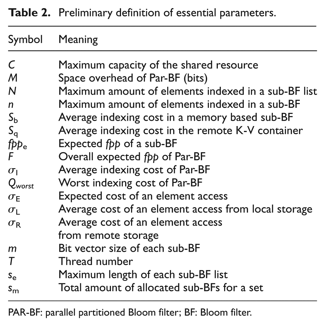
PAR-BF: parallel partitioned Bloom filter; BF: Bloom filter.
2.1. Using an index in data-intensive distributed applications
A typical data-intensive distributed computing framework architecture usually separates the compute and storage resources into two cliques: compute nodes and storage nodes, both of which are interconnected by a shared network infrastructure. The cluster of the separated disks are virtually managed and provides a universal namespace by distributed file system (e.g HDFS in Hadoop). Following up the customized scheduling, the compute nodes selectively read the to-be-processing data from the storage nodes and then saving back the processed results to the storage nodes. Through index techniques, the redundant data can be directly retrieved from local store of its compute node rather than conventionally being read from remote storage nodes. Taking a simple example, a target processing job, which is assigned to be processed in a compute node A, requests for three data blocks, X, Y, and Z. Block X has been stored in the local storage of A. Meanwhile, the index of A reports that X has been stored locally. As a result, only blocks Y and Z are read from the remote storage.
Virtualization is a key feature for a cloud-based computing framework. Virtualization enables the aggregation of multiple decentralized physical disk devices into a shared, flexible logical volume pool for centralized and elastic management. However, dynamic resource allocation leads to the expected number of elements to be stored unpredictably. For instance, as shown in Figure 1, suppose there are V disjointed and independent sets {X1, X2, …XV}. All the sets are competing for a limited and shared pre-allocated space which can store C elements at most. The major challenge is how much space should be preassigned to each Xi, 1 < i < V. We denote the space allocated to set Xi as Ci. Thus, we have equation (1). As a result, the combination value of the formalized V-tuples (C1, C2, …CV) is
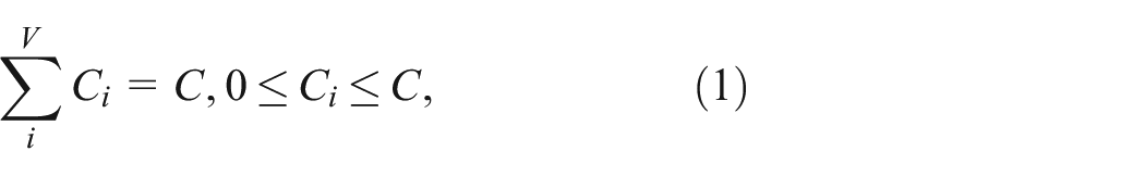
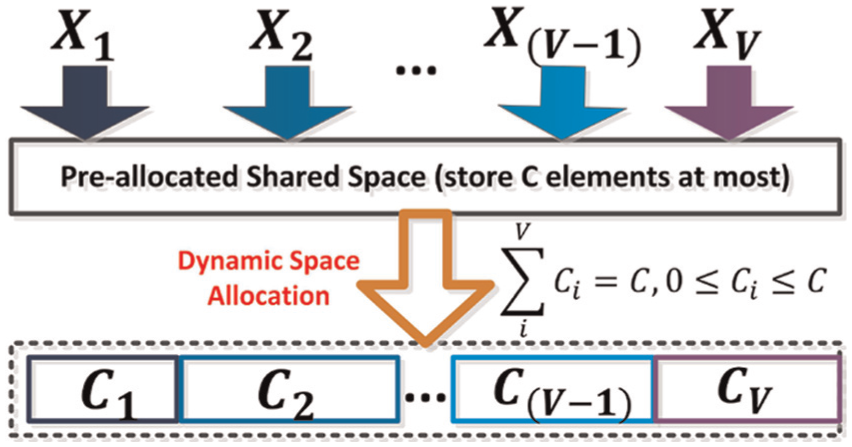
The size allocated to each Xi may change dynamically when V disjointed and independent sets
We summarize the three indexing properties for dynamic sets in data-intensive distributed computing circumstances as follows:
2.2. BFs for dynamic data sets
Hash Table is the most common data structure for indexing. However, implementing a hash table is not appealing in size-constrained and expensive memory since it requires overproportioning to guarantee that all table entries fit. Moreover, hash collisions (i.e. different entries have the same mapping position) incurs extra memory overhead (e.g. linear chaining) to handle them and deteriorate the indexing throughput (e.g. from the expected O(1) time to the worst O(n) time).To achieve both space and time efficient, the perfect universal hash functions 1 in a hash table can be optimally precalculated only when the key universe of the target set is foreseeably limited (Fredman et al., 1984). Whereas, collisions are always unexpectedly happened in a dynamic data set when the key universe is nearly infinite (Dietzfelbinger et al., 1994). Although some improved hashing solutions, such as Cuckoo Hashing (Pagh and Rodler, 2004), have been advised for dynamic sets, the collision is still considered as one of the main performance bottleneck in hashing.
Figure 2 provides a brief example of a standard BF. A standard BF for representing a data set
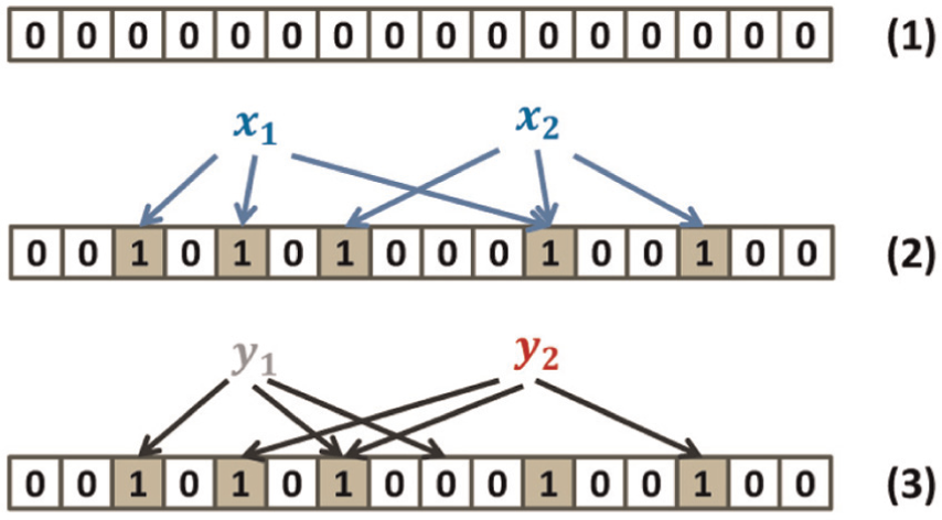
An example of a BF. m is set to 16 bits, all the bits are initialized as 0 in (1). Each element xi is hashed k = 3 times, with each hashing position is set to 1, such as the mapping positions of x1 are 2, 5, 11 in (2). The item y1 cannot be in the set X since a 0 is found at one of its mapping position. The mapping positions of item y2 are previously marked by x1 and x2, the BF has yielded a false positive in (3). BF: Bloom filter.
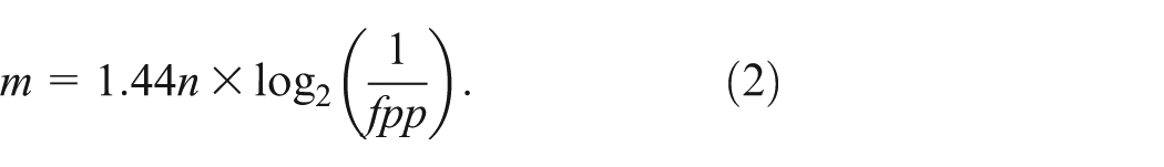
The expected fpp in a BF can be tuned in a sufficient and small range to meet indexing requirement with high-performance and low-memory overhead. Equation (2) denotes the mathematical relationship among variants m, n, and k. For example, an inline deduplication process (Zhu et al., 2008) contains 4×10⁹ unique chunks whose average size is 1 kB (The total data size is 4 TB). Assuming that each fingerprint (FP; key) of a chunk is generated by 16-byte MD5, at least 64 GB of memory for the full index is consumed in the hash table. Whereas, only 8.64 GB of memory is needed for indexing all of these chunks when the fpp of a standard BF is expected to 1/210 (≈0.0976%). Moreover, the performance drawback of hash collisions can be conditionally avoided in a BF. Counting BF (CBF) is proposed by Fan et al. (2000) for solving the problem that a standard BF dose not support element deletions. Each mapping entry in a CBF is a small counter bit rather than a single flag bit. It has been revealed that 4 bits per counter always suffice for most applications since the probability of counter overflow (≥16)can be neglected.
Neither standard BF nor CBF takes dynamic sets into consideration, while SBF and DBF are two methods to support dynamic sets as shown in Figure 1. As depicted in Figure 3, the basic idea for supporting dynamic sets is dividing the shared BF space into a certain number of sub-BF units. A new sub-BF (BFs) will be allocated into the sub-BF list of a set Xi for new insertions when all the previous sub-BFs {BF1, …, BFs−1} are full. For an element x, the membership query in set Xi will iterate its corresponding lists and return true only if x really exists in any one of sub-BFs. We summarize the characteristics of SBF and DBF as follows.
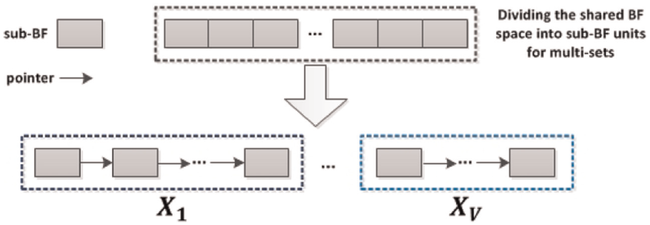
The sub-BF unit is the fundamental BF-based data structure for supporting dynamic sets. BF: Bloom filter.
2.2.1. Dynamic BF
A DBF consists of s homogeneous standard (or counting) sub-BFs. “Homogeneous” indicates both the size and the k bit-mapping hash functions are exactly the same in each sub-BF in order to support useful bit vector-based algebra operations: union, intersection, and halving (Broder and Mitzenmacher, 2004). Suppose we have two sets S1 and S2. Two homogenous BFs B1 and B2 are used to represent the element membership of S1 and S2, respectively. The algebra operations between S1 and S2 are listed as follows.
2.2.2. Union
A BF B that represents the set union
2.2.3. Intersection
A BF B that represents the set intersection
2.2.4. Halving
It is a special case of union. For example, if the BF B with size m is divisible by 2, halving can be done by bitwise OR between the first and second halves. Thus, the size of B becomes m/2, and each modified bit position of element x is calculated by
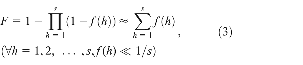
However, the main problem of DBF is that there is no mechanism to control the overall false positive rate F. Let f (h) denote the fpp of a sub-BF BFh. F is calculated according to equation (3). In DBF, F equals to the probability of any one of the sub-BFs occurring a false positive during an element membership query. Assuming each sub-BF can index n elements at most. Thus, we have
2.2.5. Scalable BF
An SBF is made up of a series of heterogeneous sub-BFs. Both m and k of each sub-BF are different. The key idea is that each successive sub-BF is created with a tighter maximum error probability on a geometric progression according to equation (4), where r, 0 <r < 1 is the tight factor.

Thus, the compounded probability over the whole series is in convergence to
Increasing the average consumed bits of a key in BFh by
No support of BF-based algebra operations so as to simplify resource management.
Recalculating mapping positions of each sub-BF iteration for an element membership query. The cost is
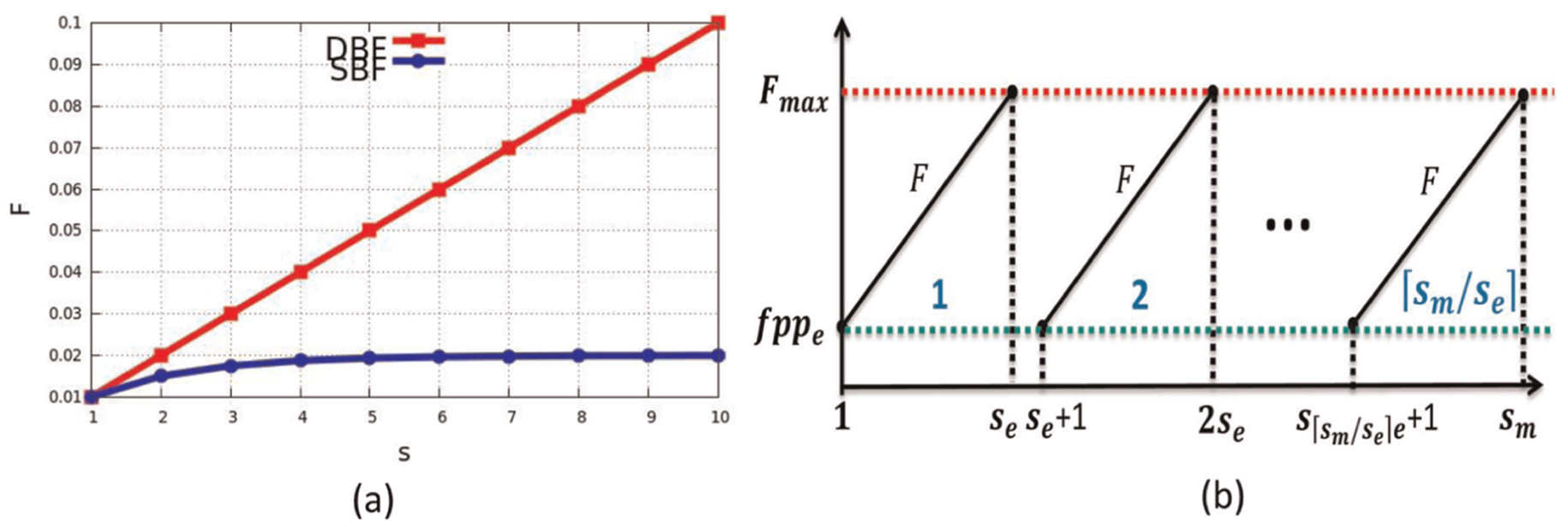
(a) An example of F value growth comparison between DBF and SBF, f(1) = 0.01, r = 0.5 in SBF. (b) Our recommended Par-BF design,
2.3. Performance/cost-driven initializations of a BF
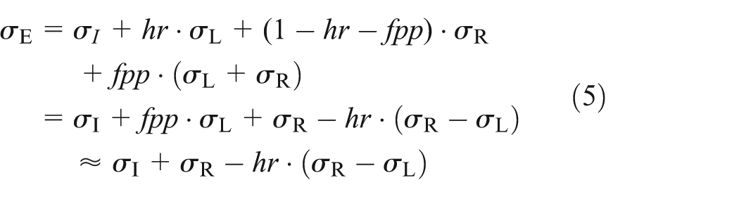
As illustrated in Figure 5, there are three states of an element x membership query including In, Not in, and False Positive. Suppose element x is requested for further processing. Through BF-based indexing, x is identified whether existed in the local store first, in terms of either K-V store or cache manner containing a subset of the data. The average indexing cost is roughly denoted as

Three states of element membership query in a BF. BF: Bloom filter.
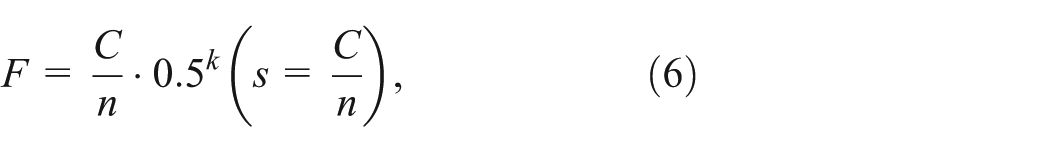
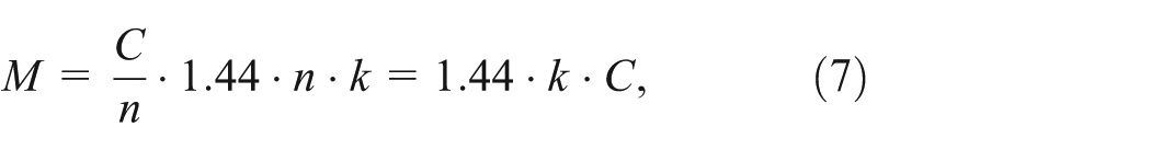
There is a trade-off between performance and memory overhead in designing a BF. The overall fpp plays a negative effect on the performance. As in equation (6), both n (capacity) and k (mapping functions) of each homogenous sub-BF are positive factors to reduce the F value (derived from equation (3), where
The expected
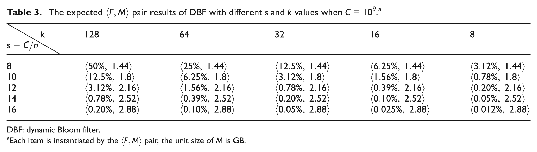
DBF: dynamic Bloom filter.
Each item is instantiated by the
3. Design of Par-BF
3.1. Principles
The design of Par-BF is shown in Figure 6. The shared BF space of set Xi is divided into a certain number of sub-BF lists. The total number of sub-BF lists is

The design of Par-BF. PAR-BF: parallel partitioned Bloom filter.
The expected upper bound value of fpp in each sub-BF list is set to
From Figure 4(b), Par-BF has the following two features: (1) the maximum fpp of each matching thread is limited to Fmax and (2) the list size for matching iteration is limited so as to improve query throughput. The time cost of iterating a list contains sm sub-BFs is
3.2. Element operations
To EXPLOIT the hierarchical relationship of different components in Par-BF, we define three as shown in Figure 7.

Flow charts of the three element operations in Par-BF. There are totally
3.1.1. Lookup
There are maximum
3.1.2. Insertion and deletion
For both insertion and deletion of an element x, the multi-thread lookup operation often locates the corresponding sub-BF in advance. The key of element x insertion is mapped into the corresponding position of an active sub-BF whose amount of the indexed elements is less than the maximum n in a sub-BF. If there is no active sub-BF, a new sub-BF and its corresponding data container will be allocated for new element insertions. We use CBF for each sub-BF to support element deletions. For element x deletion, each mapping position of its corresponding sub-BF is decreased by 1.
3.2. Memory optimizations in Par-BF
Although CBF supports element deletions, the space requirement of a CBF is three times more than its original BF, because it stores a 4-bit counter rather than 1-bit flag in each position of the mapping array. We propose building CBFs in a relative slow block device (compared with memory) to keep track of element update, while keeping the transformed standard BFs in memory. As shown in Figure 8(a), each sub-CBF will be transformed into the corresponding BFs according to Figure 8(b) method. Then, we can update the position bit between a standard sub-BF and its corresponding sub-CBF. However, this transformation method is only advised for read-mostly workloads due to the synchronization cost of element update between CBF and BF.
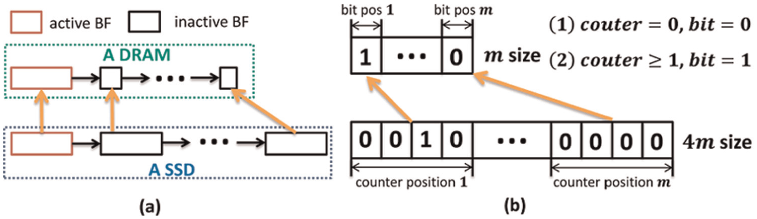
(a) Transformed standard sub-BFs instead of sub-CBFs will exist in DRAM for fast matching. (b) The transformation method. BFs: Bloom filters; DRAM: dynamic random-access memory.
To reclaim the free space after element deletions and make better use of memory space, Par-BF uses the union algebra operation to do garbage collection. A union operation mainly contains two steps.
Sorting each sub-BF in a set by the total number of stored elements ascendingly,
If
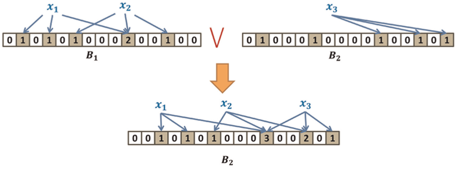
An example of the union operations between two sub-BFs. Each BF is initialized as a CBF. There are 16 mapping entries (m = 16 × 4 bits), k = 3, and n = 3. BFs: Bloom filters; CBF: counting Bloom filter.
3.3. Parameter initializations
Some essential parameters of Par-BF can be tuned to meet the requirement of both performance and memory overhead. The appropriate values can be delibrately derived from the lookup performance analysis in Par-BF.
3.3.1. Lookup cost analysis
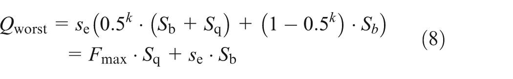
Suppose that the computing resources are fairly shared by each nondistinctive thread. When the element x does not exist, iterating the sub-BF list of a matching thread from the head to the tail for an element x membership lookup costs the most time. We denote the worst time cost as Qworst. Equation (8) shows the expected Qworst, where the expected probability of a full sub-BF returns a wrong match result
3.3.2. Parameter tunings
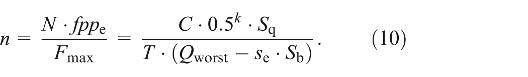
Assigning an appropriate number of threads is very important to obtain good performance for a multi-threaded application running on a multi-core system. Few threads may not fully utilize multi-core resources. While if we assign more threads than the hardware can support (which is called oversubscription) for task running, the context switching and the lock mechanism will decrease the performance. Thus, we need to create a suitable number of threads for indexing. A simple and effective way is that the thread number is equal to that of CPU cores (Pusukuri et al., 2011). For example, the Thread library of C++ 11 uses the caller std:: thread:: hardware_concurrency() to return the number of threads that can truly run concurrently for a given execution of a program, which is equal to the number of CPU cores in default. This indicates that N is equal to C/T. T is also equal to the maximum number of sub-lists (each thread is responsible for a sub-list matching process). We can conduct equation (9) since
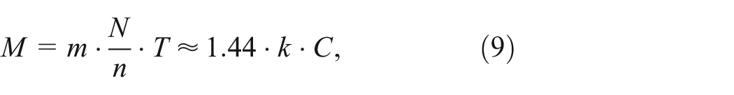
As
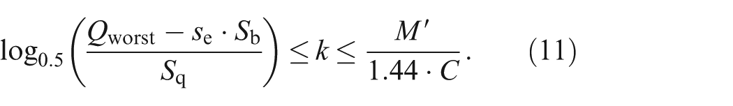
We summarize the results of some parameters in Table 4. From equation (9), we conclude that if the maximum space overhead is limited by M′, the inequality
Results of some essential parameters in Par-BF.
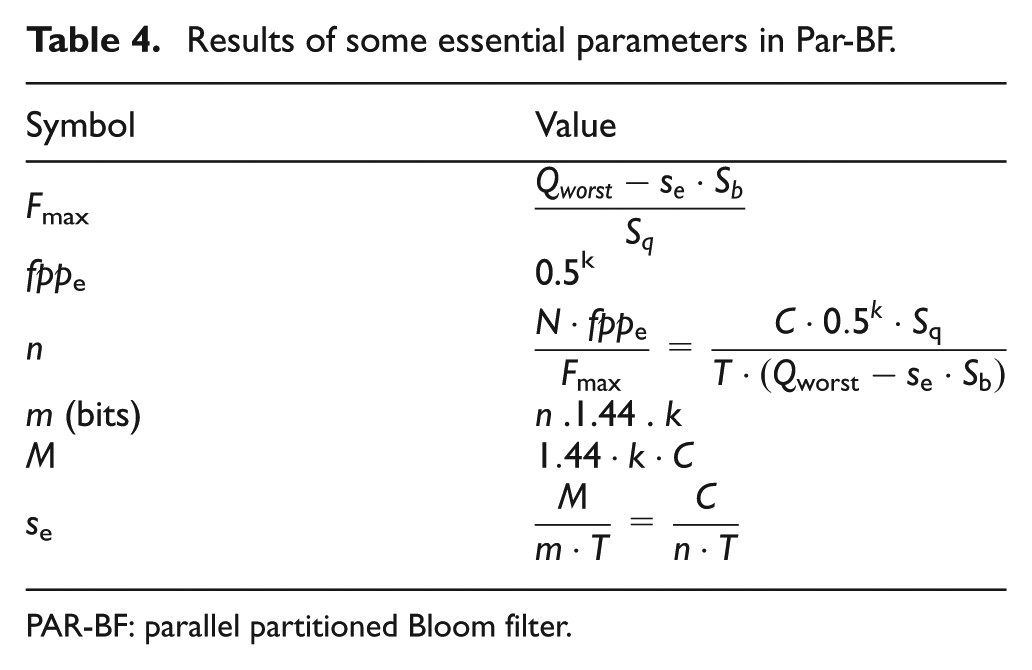
PAR-BF: parallel partitioned Bloom filter.
4. Evaluation
We evaluate and verify the design of Par-BF using an example of typical distributed I/O intensive process, network redundancy elimination (NRE). NRE aims to identify and eliminate duplicate chunks that are repeated across network links. The Par BF-based NRE has been established in our network function virtualization prototype in Openstack (Ge et al., 2014). Briefly speaking, the NRE process is to segment a transferred data stream into a certain amount of data chunks according to a fixed- or variable-size chunking policy (Anand et al., 2009). Those chunks are stored in a local store for future reuse instead of reading them from the remote data servers. The efficiency of NRE is in direct proportion in duplicated chunk identification through Par-BF. Specifically, we focus on four aspects: (1) the effects of parameter tuning to meet performance/cost trade-off in a heterogeneous environment; (2) the lookup performance in DBF, SBF, and Par-BF; (3) the efficiency of garbage collection to reduce memory overhead; and (4) the performance effect of choosing different thread number in Par-BF.
4.1. Experiment setup
As illustrated in Figure 10, there are three nodes, A, B, and C, to do NRE services when configuring heterogeneous local store(s) to meet the SLA of each NRE service. The subset of chunks are managed in a cache manner in each node. The local store of nodes A, B, and C is built upon only memory, both memory and Flash, and only Flash, respectively. LRU is set as the default cache replacement algorithm. The role of Par-BF is to quickly determine the source side of a requested chunk from either the local node or the remote data container. CBF is the fundamental unit of Par-BF to support chunk deletions due to the replacement operations. We evaluate Par-BF on a Ubuntu 13.02 64-bit server. The basic hardware environment is described in Table 5. As given in Table 6, following equation (5),
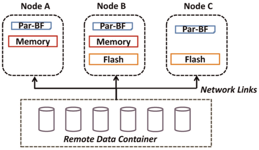
Overview of the experimental simulation diagram.
The composition of our testing heterogeneous environment.
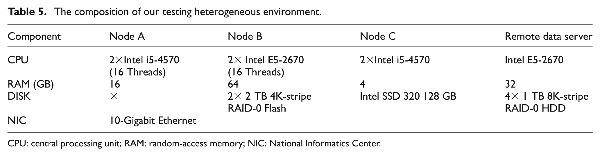
CPU: central processing unit; RAM: random-access memory; NIC: National Informatics Center.
Measurements of I/O costs in our testing heterogeneous environment.
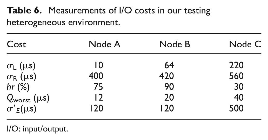
I/O: input/output.
We set T =16×2 in default, which is equal to the number of CPU cores in each compute node. Three major experimental components are configured as follows.
4.1.1. Generating FP
We use a 128-bit variant of Murmurhash (Appleby, 2009) to generate a FP (as key) to represent a chunk. The former [0, 63] bits of the generated 128 bits are considered as the final key considering the trade-off between key space saving and key collision. FP is considered as the hint to get the target chunk from the remote container rather than directly comparing chunks.
4.1.2. Generating k random hash functions for each sub-BF
Adam Kirsch and Michael Mitzenmacher (Kirsch and Mitzenmacher, 2006) have proved that applying two independent hash functions, h1(x) and h2(x), to simulated additional hash functions as the form of
4.1.3. The implementation of remote key-value containers
We use Berkeley DB (BDB in short) to organize remote key-value data containers, using a B-Tree index, where each key is the FP of a chunk and the value is chunk’s content.
4.2. Data trace
We develop a software simulator to generate a key-value workload according to the principles of the Yahoo! Cloud Serving Benchmark (YCSB) (Cooper et al., 2010). YCSB uses the Monte-Carlo method to generate a typical I/O access distribution. At first, a certain amount of chunks are chosen by obeying a probability distribution from the large sample space of unique chunks. Then these chunks are organized by the trace files which are formatted as lines of chunk key: chunk content: size: operation through the colon as the delimiter. The operation is instantiated by one of the three operations, read, write, and delete. Finally, each trace file is formatted as lines of timestamp: file name to simulate the user’s behavior.
For simplicity, each data flow for satisfying clients request is based on the whole file granularity. The chunk is identified as the duplicated one when it is hit in cache, otherwise, it will be read from the remote data container, and, additionally, to emulate the user behavior to request files of data sets. We generated data requests from three distinct synthetic traces, T1, T2, and T3 to simulate differentiated NRE services according to the access characteristics of practical network applications. Table 7 describes the three traces in detail. For example, the T1 trace contains 8.25×10¹² requests for 1.2×10⁹ unique chunks with 128B average request size. Nodes A, B, and C use T1, T2, and T3 to simulate data requests, respectively.
The statistics of NRE traces. a
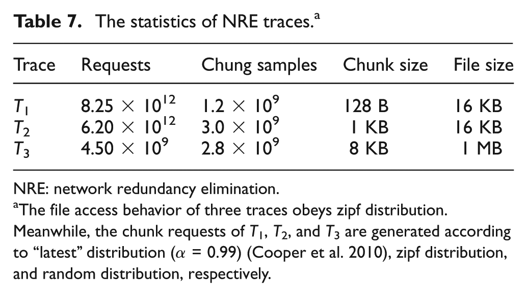
NRE: network redundancy elimination.
The file access behavior of three traces obeys zipf distribution. Meanwhile, the chunk requests of T1, T2, and T3 are generated according to “latest” distribution (α = 0.99) (Cooper et al. 2010), zipf distribution, and random distribution, respectively.
4.3. Parameter tunings
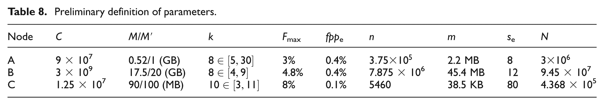
The parameters for tuning in Par-BF are given in Table 8. Node B is used as an example to analyze the progress of parameter tunings in detail. We use 3 TB Flash as the K-V store in the local side to speedup chunk reads. Thus, the overall capacity of elements (chunks), C, is 3×10⁹. The worst indexing time of Par-BF, Qworst, is measured as 20 µs (see Table 6). All sub-BFs are kept in memory so we can neglect Sb . Sq is 420 µs, which equals to
Preliminary definition of parameters.
As shown in Figure 11, the average indexing latency
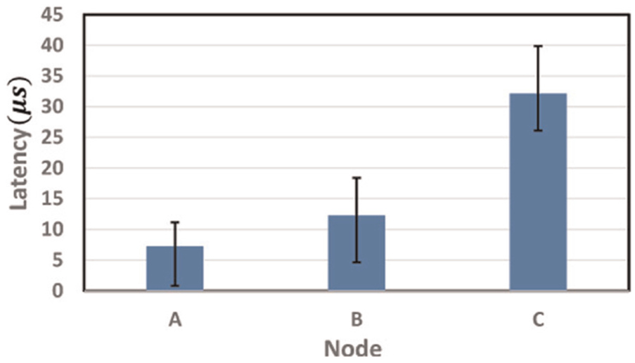
Results of measuring
Par-BF is also able to find a sweet point to balance the trade-off between high performance and low overhead. Suppose that
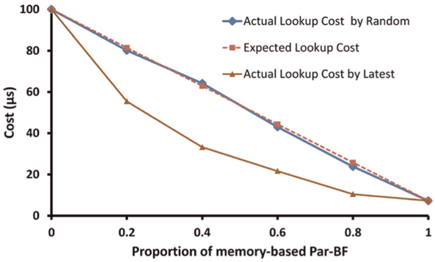
Indexing cost (latency) comparisons between the actual values and the expected value when choosing different proportion of memory overhead
4.4. The performance of Par-BF
The negative effect of a false positive slows down the overall throughput of matching. According to equation (3), fppe must be restricted in an acceptable range to meet the matching performance requirement. We record the average indexing throughput of nodes A, B, and C through three dynamic BF mechanisms, DBF, SBF, and our recommended Par-BF and the results are shown in Figure 13. Accordingly, we have the following conclusion.
The IOPS of Par-BF outperforms that of DBF and SBF, by 10× to 14× and by 3× to 8×, respectively. This is because that Par-BF always contains T matching threads to achieve parallelism.
DBF always performs the worst. There are mainly two reasons. One is that its list size is more than 15× compared with the value of Par-BF. The other results from the unacceptable false positive value
Compared with T3, maintaining temporal locality of chunk accesses in T1 and T2 can greatly increases the IOPS.
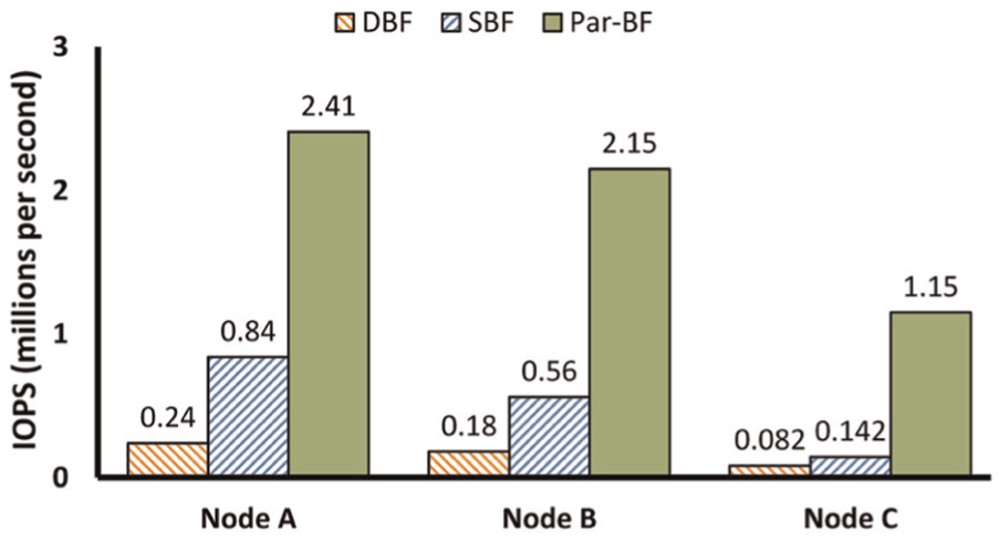
Throughput comparisons between DBF, SBF, and Par-BF through running T1, T2, and T3. The initialized r = 0.5, s = 2, and f(1) = fppe of SBF. DBF: dynamic Bloom filter; SBF: scalable Bloom filter; Par-BF: parallel partitioned Bloom filter.
4.5. Garbage collection
Figure 14 shows the memory overhead of node B without doing GC. The memory overhead of both DBF and Par-BF is less than that of SBF by about 0.75 GB. Supporting chunk deletions is the precondition to do garbage collection. As a result, CBF is advised as the basic sub-BF data structure. The space overhead of CBF is more than that of the basic BF by about 3× as usual. Figure 15 shows the benefit of GC process in the NRE process. The stored chunks are more valuable and wastes less storage space. For instance, the redundant chunks of T2 are only occupied by 21.76% without GC, whereas, this value is 48.36% with GC. This difference indicates that the GC process makes the memory space more efficient
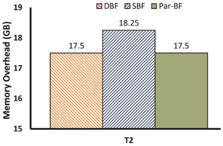
The memory overhead of using data trace T2 by the three BF policies. BF: Bloom filter.
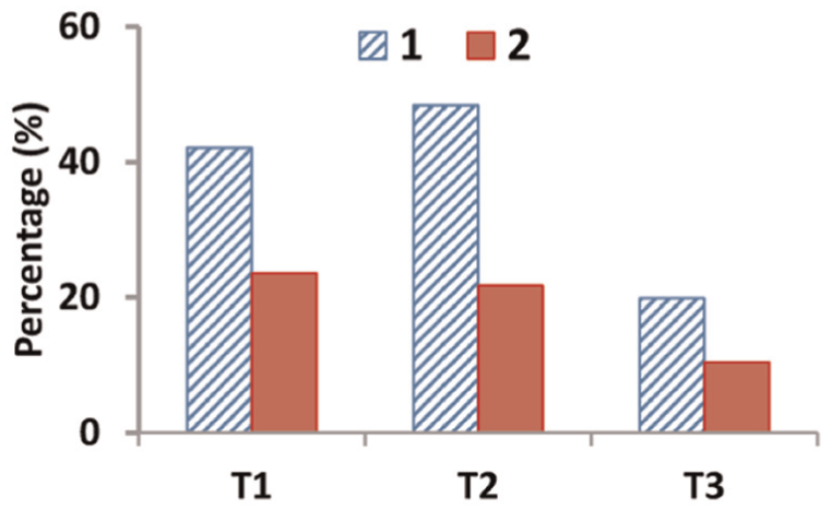
The comparison on percentage of chunk access in each trace (type “1” denotes “do GC” and type “2” denotes “do NOT GC”).
4.6. Choosing thread number
The results of Figure 16 validates the rationality of choosing thread number, T, which equals to that of CPU cores. From Table 4 and equation (10), we know that
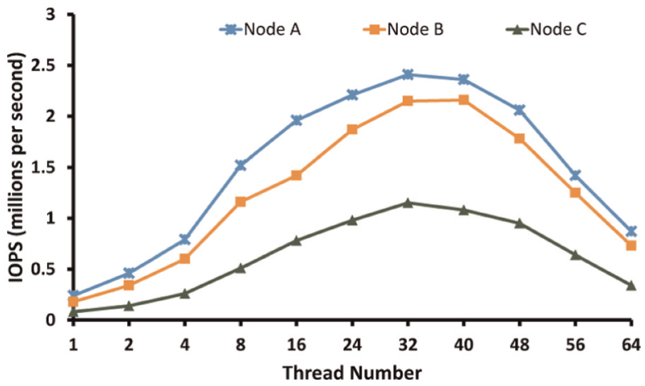
Par-BF throughput comparisons of choosing different thread number in the three nodes. PAR-BF: parallel partitioned Bloom filter.
4.7. Trade-off between memory overhead and indexing performance
As we mentioned above, the expected fppe of each sub-BF in Par-BF is relative to between memory overhead and indexing performance. From Table 4, the fppe is positive, calculated by k. As shown in Figure 17, we gave the comparisons in memory overhead and average latency by choosing four typical k value in node B. We can conclude: (1) A Par-BF with smaller k value uses less memory size but more deteriorates the average indexing latency. For example, the memory overhead is 8.78 GB and the average indexing latency is 48.6 µs when k is set to 4. In contrast, the memory overhead is extended to 52.1 GB, but the average indexing latency is reduced to 0.16 µs when k is set to 24. (2) Once a traditional hash table based on linear chaining is used as the indexing structure, the memory overhead is 48 GB to indexing all FPs of chunks, while the average latency of indexing is about 2.4 µs, which cannot be neglected due to hash collisions. (3) Finally, k = 8 is recommended as given in Table 8 to meet the trade-off between memory overhead (17.5 GB) and indexing performance (12.25 µs).
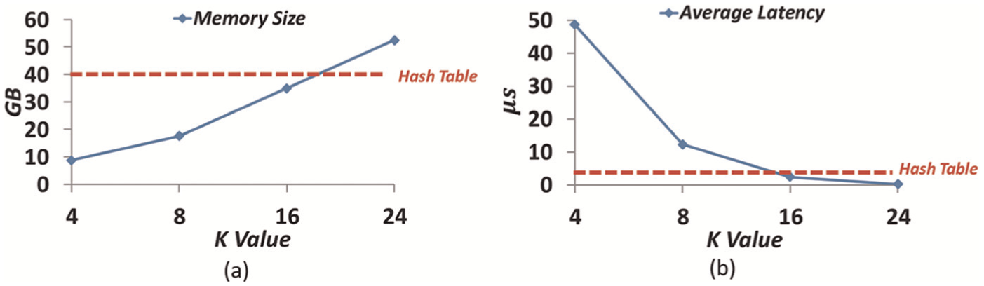
Comparisons with choosing different k in Par-BF in node B: (a) memory overhead and (b) average latency. Traditional hash table based on linear chaining is used as the baseline. PAR-BF: parallel partitioned Bloom filter.
5. Related work
Our work is built upon previous great work as follows.
5.1. Application
Guided by the space-efficient property of BFs, which is first given in 1970s (Bloom, 1970), the BF-based indexing becomes more and more popular for fast matching applications. Anand et.al. (2009) proposed BF as the index to identify FP matches in various of NRE processes. Zhu et al. (2008) used a BF for backup deduplication, called Summary Vector, as the summary data structure to test whether a data chunk is a duplicated one. Debnath et al. (2010) designed a disk-presence BF in RAM to record keys destaged to hard disk so that hard disk access latencies can be avoided when lookups are done on nonexisting keys in a large-scale deduplication system. BF-based index are also used in IP routing (Li et al., 2011; Song et al., 2005; Yu et al., 2009). Broder and Mitzenmacher wrote an excellent survey on network applications of BFs (Broder and Mitzenmacher, 2004). Meanwhile, there are some excellent literatures (Anand et al., 2010; Debnath et al., 2011; Lu et al. 2012), in designing flash-based BF to provide a new dimension of trade-off with BF access times to reduce RAM space usage. Specially, BF-based joins, Bloomjoin have been widely well studied (Babb, 1979; Lee et al., 2012; Michael et al., 2007; Mullin, 1990) to optimize distributed query execution in a distributed database (e.g. Hive in Map/Reduce frameworks).
5.2. Variants of BF
Many variants based on basic BF technique have been proposed in the previous research. The d-left CBF(Bonomi et al., 2006) divides a hash table into d sub-tables which have the same size. The d-left CBF offers the same functionality as a CBF, but uses less space, generally saving a factor of two or more. Compressed BF (Mitzenmacher, 2002) improves delivery efficiency when a BF is passed in a message between distributed nodes. The hierarchical BF (Shanmugasundaram et al., 2004) is a data structure to support multiple substring (block-size granularity) matchings. The spectral BF (Cohen and Matias, 2003) mainly supports membership query in multi-sets. Bloomier filters (Chazelle et al., 2004) allows association of values with a subset of the domain elements, which are implemented using a cascade of BFs. Weighted BF (Jehoshua et al., 2006) exploits the priori knowledge of the frequency of an element request by varying the each mapping function popularity degree. Hao et.al. prposed a partitioned hashing technique to select hash functions that set fewer bits (Hao et al., 2007). Although their experimental results show that they can improve the performance by 10-fold compared with standard contructs, it is not applicable for dynamic environments. Tarkoma et.al. gave a comprehensive survey on reviewing over 20 variants and discussing their applications in distributed systems (Tarkoma et al., 2012). The most closely related literatures of our work are the DBF (Guo et al., 2010) and the SBF (Almeida et al., 2007). However, both still face some challenges on system performance and memory overhead for indexing a large-scale dynamic data set aforementioned.
6. Conclusion and future work
Multiple independent sets contesting with a restricted shared resource is universe in multitasks-based computer systems. As shown in Table 1, both DBF and SBF still face the challenge by indexing dynamic data sets with low memory overhead but achieving high performance. In order to overcome this challenge, we design a new BF, called Par-BF, which can tune the essential parameters by a group of formulas. We validate our Par-BF design via trace-driven evaluation in a practical application. Through supporting parallel fast matching with suitable thread number, the performance of Par-BF outperforms that of both DBF and SBF. Moreover, Par-BF costs less memory than DBF and SBF for the union algebra operation in Par-BF reduces memory wastage .
6.1. Future work
Due to our limitations, an interesting problem on exploiting Par-BF in hardware accelerators, such as graphics processing units, field-programmable gate array, is not discussed in this article. We intend to use more benchmarks to evaluate Par-BF and validate more applications, especially for I/O-intensive scientific computing. The code of Par-BF is openly available for future study at https://github.com/ironliuyi/Par-BF.
Footnotes
Acknowledgements
We authors would like to thank the anonymous reviewers for their valuable feedbacks to improve this article. We also appreciate Dr Liang Zhang and other researchers from Huawei Corporation for their support.
Declaration of Conflicting Interests
The author(s) declared no potential conflicts of interest with respect to the research, authorship, and/or publication of this article.
Funding
The author(s) disclosed receipt of the following financial support for the research, authorship, and/or publication of this article: This work is partially supported by the following NSF awards: 1439622, 1305237, 1421913, 1217569, and 1115471.
Notes
Author biographies
Yi Liu is currently a researcher in Huawei. In 2015, he received his doctoral degree in Computer Application Technology from Shenzhen Institutes of Advanced Technology, Chinese Academy of Science, China. In 2008, he received his bachelor’s degree in computer science at National University of Defense and Technology, China, and in 2011, he received his master’s degree in software engineering at Peking University, China. His current research interests include SSD storage techniques and deduplication in networks and backup systems.
Xiongzi Ge is currently a PhD student at the Department of Computer Science and Engineering, University of Minnesota, Twin Cities. He received his BE and PhD degrees in computer science from Huazhong University of Science and Technology, China, in 2005 and 2012, respectively. He was a senior software engineer in Shenzhen Cloud Computing Center from 2011 to 2013. He was a visiting scholar in the Shenzhen Institutes of Advanced Technology, Chinese Academy of Sciences, from 2009 to 2011. He was a visiting student of the Digital Technology Center (DTC), in University of Minnesota, from 2008 to 2009.
David Hung-Chang Du is currently the Qwest Chair Professor of Computer Science and Engineering at University of Minnesota, Minneapolis. He is the Center Director of the NSF multi-university I/UCRC Center of Research in Intelligent Storage (CRIS). In addition to NSF, CRIS is currently sponsored with 11 companies with 15 sponsored memberships. He was a Program Director (IPA) at National Science Foundation CISE/CNS Division from March 2006 to August 2008. At NSF, he was responsible for NeTS (Networking Research cluster) NOSS (Networks of Sensor Systems) Program and worked with two other colleagues, Karl Levitt and Ralph Wachter, on Cyber Trust (Internet Security) Program. In 2008, he was also assigned to CSR (Computer System Research) Cluster for handling research in computer systems. He received his BS degree in mathematics from National Tsing-Hua University (Taiwan) in 1974 and MS and PhD degrees from the University of Washington (Seattle) in 1980 and 1981, respectively. He joined the University of Minnesota as a faculty since 1981. He also has been a visiting professor in Germany, Korea, Singapore, Hong Kong, and Taiwan.
Xiaoxia Huang is currently a professor in Shenzhen Institutes of Advanced Technology, Chinese Academy of Sciences, China. She is the Deputy Director of the Center for Real-Time Monitoring and Communications Technologies (RTT). Her research interests include cognitive radio networks, smartphone applications, wireless sensor networks, and wireless communications. She received her BE and ME degrees in electrical engineering from Huazhong University of Science and Technology, China, in 2000 and 2002, respectively, and the PhD degree in electrical and computer engineering from the University of Florida in 2007.