
Abstract
Ultra-large–scale simulations via solving partial differential equations (PDEs) require very large computational systems for their timely solution. Studies shown the rate of failure grows with the system size, and these trends are likely to worsen in future machines. Thus, as systems, and the problems solved on them, continue to grow, the ability to survive failures is becoming a critical aspect of algorithm development. The sparse grid combination technique (SGCT) which is a cost-effective method for solving higher dimensional PDEs can be easily modified to provide algorithm-based fault tolerance.
In this article, we describe how the SGCT can produce fault-tolerant versions of the Gyrokinetic Electromagnetic Numerical Experiment plasma application, Taxila Lattice Boltzmann Method application, and Solid Fuel Ignition application. We use an alternate component grid combination formula by adding some redundancy on the SGCT to recover data from lost processes. User-level failure mitigation (ULFM) message passing interface (MPI) is used to recover the processes, and our implementation is robust over multiple failures and recovery (processes and nodes).
An acceptable degree of modification of the applications is required. Results using the 2-D SGCT show competitive execution times with acceptable error (within 0.1% to 1.0%), compared to the same simulation with a single full resolution grid. The benefits improve when the 3-D SGCT is used. Experiments show the applications ability to successfully recover from multiple failures, and applying multiple SGCT reduces the computed solution error. Process recovery via ULFM MPI increases from approximately 1.5 sec at 64 cores to approximately 5 sec at 2048 cores for a one-off failure. This compares applications’ built-in checkpointing with job restart in conjunction with the classical SGCT on failure, which have overheads four times as large for a single failure, excluding the recomputation overhead. An analysis for a long-running application considering recomputation times indicates a reduction in overhead of over an order of magnitude.
Keywords
1 Introduction
Today’s largest high-performance computing (HPC) systems consist of thousands of nodes which are capable of concurrently executing up to millions of threads to solve complex problems within a feasible period of time. The nodes within these systems are connected with high-speed network infrastructures to minimize communication costs (Ajima et al., 2009). Significant effort is required to exploit the full performance of these systems. Extracting this performance is essential in different research areas such as climate, the environment, physics, and energy, which all are characterized by the complex scientific models they utilize.
In the near future, besides exploiting the full performance of such large systems, dealing with component failures will become a critical issue. Generally, the failure rate of a system is roughly proportional to the number of nodes of the system (Schroeder and Gibson, 2006). For instance, a 382-days study on the 557 Teraflops Blue Gene/P system with 163,840 computing cores at Argonne National Laboratory showed that it experienced a failure (hardware) every 7.5 days (Snir et al., 2014). Since the typical size of HPC systems is becoming larger as we approach exascale computing, the rate at which they experience failures is also increasing (Gibson et al., 2007). A study by Snir et al. (2014) assumed the mean time to failure of an exascale system as 30 min. The set of possible solutions to deal with such frequent failures, as reported in Snir et al. (2014), is divided into three categories: the hardware approach, the system approach, and the application approach.
The hardware approach will add additional hardware in an exascale system to deal with failures on the hardware level. Although this will require the least effort in porting current applications, it will incur additional power consumption in the system. Moreover, as the hardware in exascale system becomes more complex, the software will become more complex and hence error prone. In this scenario, new complexities arise in the system due to the introduction of additional hardware.
In the system approach, a combination of hardware and system software is used to handle faults in a manner that becomes transparent to the application developers. This approach will require no change in application codes and is therefore equivalent to the hardware approach from the viewpoint of application developers. Although the relative cost of hardware changes versus system software changes will dictate preferences between the hardware approach and the system approach, this may add additional complexities in the system and, hence, may increase its energy consumption.
The application approach requires application developers to handle resilience as part of their application code. Although this approach seems more invasive from the viewpoint of the application developers, it may reduce the cost of exascale platforms and their energy consumption. Moreover, application developers have more options to select the most appropriate resiliency strategy for their applications.
Thus, there is an urgent need to develop large-scale fault-tolerant (FT) applications using application-level resiliency. Traditionally, large-scale applications use the message passing interface (MPI) (Message Passing Interface Forum, 1993), which is a widely used standard for parallel and distributed programming of HPC systems. However, the standard does not include methods to deal with one or more component failures at run-time. In order to address this problem, FT-MPI (Fagg and Dongarra, 2000) was introduced to enable MPI-based software to recover from process failure (see Ali and Strazdins, 2013, for details). However, the development of FT-MPI was discontinued due to the lack of standardization. Recently, the MPI Forum’s Fault Tolerance Working Group began work on designing and implementing a standard for user-level failure mitigation (ULFM) (Bland, 2013a), which introduces a new set of tools to facilitate the creation of FT applications and libraries. These tools provide MPI users the ability to detect, identify, and recover from process failures. It is a great opportunity for application developers to use these tools to make their applications FT.
Currently, there is a lack of practical examples that demonstrate the range of issues encountered during the development of FT applications. Moreover, the amount of literature detailing the implementation and performance of the proposed standard is very limited. Some of the work that is available assumes a fail-stop process failure model, that is, a failed process is permanently stopped without recovering and the application continues to work with the remaining processes (Hursey et al., 2007). However, this model is not adequate for all applications. For example, some applications do not tolerate a reduction of the size of the MPI communicator and, thus, require recovery of the failed processes in order to finish the remaining computation successfully.
There appears to be an even greater lack of research on how to make existing, complex, and widely used parallel applications FT. In this article, we demonstrate how three existing applications (the Gyrokinetic Electromagnetic Numerical Experiment (GENE) plasma simulation code, the Taxila Lattice Boltzmann Method (LBM) application code, and the Solid Fuel Ignition (SFI) application code) can be made FT using ULFM MPI and a form of algorithm-based fault tolerance obtained via modification of the sparse grid combination technique (SGCT). Our implementation includes the restoration of failed processes and MPI communicators on either existing or new (spare) nodes.
There are different kinds of faults that may occur in a system. Based on the symptoms and consequences of each category, different types of strategies are followed to handle them. The level of effort needed to identify and handle them may vary from one category to the other. Of many categories, some common types of faults are transient (faults that occur once and then disappear), intermittent (faults that occur, then vanish again, then reoccur, then vanish), permanent (faults that continue to exist until the faulty component is repaired or replaced), fail-stop (faults that define a situation where the faulty component either produces no output or produces output that clearly indicates that the component has failed), and Byzantine (faults that define a situation where the faulty component continues to run but produces incorrect results). Although it is desirable that an FT technique will be able to handle all types of faults, but in practice, it is too hard to design and implement such a technique.
In this work, we are not handling all the above-mentioned types of faults. The scope is narrowed down to handle only the permanent or fail-stop type of faults. More specifically, we are looking at the problem of recovering from the application process failures, caused by the hardware or software faults, from within the application.
The contributions of this article are to (i) detail how a scalable SGCT algorithm can be integrated into three existing and complex applications to make them highly FT; (ii) evaluate the effectiveness of applying SGCT on two of these applications which are, to our knowledge, the first attempt; (iii) evaluate the capabilities of ULFM MPI to recover from single or multiple real process/node failures for a range of complex applications; (iv) perform a detailed experimental evaluation of this work including time and memory requirements and parallelization on the non-SGCT dimensions; and (v) perform an analysis of result errors in terms of number of failures, load balancing, overhead due to computing extra unknowns for fault tolerance, and an analysis of recovery overheads. The latter includes a comparison with traditional checkpointing on application simulations using a non-FT SGCT.
The article is organized as follows. Section 2 provides a discussion of related research. Background relating to this research is discussed in Section 3. The experimental methodology is described in Section 4, followed by a discussion of general methodology for SGCT integration in Section 5. Sections 6, 7, and 8 describe the existing GENE application, Taxila LBM application, and SFI application, respectively, including how they were adapted to become FT using a highly scalable SGCT algorithm and experimental evaluation. A load-balancing technique and its evaluation are presented in Section 9. Failure recovery overheads for shorter and longer computations, overheads incurred to achieve fault tolerance in the SGCT, and repeated failure recovery overheads are described in detail in Section 10. Finally, conclusions are given in Section 11.
2 Related work
Our present work lies at the intersection of four active research and development areas—parallelization of the SGCT, recovery of process and node failures with ULFM MPI, algorithm-based fault tolerance (ABFT) techniques, and evaluation of the effectiveness of applying SGCT to the GENE plasma micro-turbulence code, the Taxila LBM code, and the SFI code. Below we summarize and contrast work most closely related to ours.
A technique for replacing only a single failed process in the communicator and matrix data repair for a QR Factorization problem was proposed by Bland (2013). Process failure was handled by ULFM MPI, and data repair was accomplished using a reduction operation on a checksum and remaining data values. The author analyzed the execution time and overhead on a fixed number of processes in the presence of a single process failure. A detailed performance analysis of the recovery mechanism for multiple process failures, however, was not presented. Nor was the technique applied to a varying number of processes in other realistic parallel applications. A detailed performance evaluation of different ULFM MPI routines used to tolerate process failures was found in Bland et al. (2012).
An FT implementation of a multilevel Monte Carlo simulation that avoids checkpointing or recomputation of samples was proposed in Pauli et al. (2013). It used ULFM MPI to recover the communicator after failures by sacrificing its original size. A periodic reduction strategy was incorporated to all the samples unaffected by failures in the computation of the final result and simply excluded the samples affected by failures. The periodic communication/reduction is likely to be costly across multiple nodes, and the experimental results relating to multiple nodes were not provided. Reconstruction of the faulty communicator was not considered, nor were data recovery implemented.
Local Failure Local Recovery (LFLR) was proposed in Teranishi and Heroux (2014). It inherited the idea from diskless checkpointing (Plank et al., 1998) in which some spare processes accommodated a space for data redundancy and local checkpointing. This allows an application developer to perform a local recovery without disrupting the execution of whole application when a process fails. The idea is to split the original communicator into several group communicators and dedicate a spare process for each group to store the parity checksum of the corresponding group. In the event of a single process failure, the corresponding spare process replaces the failed one with ULFM MPI and recover the lost data locally from the local memory checksum. It requires local checksum to be updated periodically, which seems to be costly. Spare processes are used in the LFLR approach to handle only single process failure. In our approach, we are also using extra processes for a small amount of redundant computations, but we are able to tolerate multiple process failures.
A customized run-time–based simplified programming model called Fault-Tolerant Messaging Interface (FMI) was designed and implemented in Sato et al. (2014) to improve the resilience overheads of the existing multilevel checkpointing method and MPI implementations. The semantics needed to write applications were similar to MPI, but the resiliency of applications was ensured by the FMI interface. Scalable failure detection with the help of a log-ring overlay network, fast in-memory checkpointing on spare nodes, and dynamically allocating spare compute resources in the event of failures were proposed. Although the main objective of providing resiliency to applications is the same, we are applying an ABFT for the approximate recovery of multiple failures, rather than the exact recovery through diskless checkpointing. Our failure detection and process recovery techniques are also different.
Early work in the parallelization of the SGCT for Laplace’s equation and the 3-D Navier–Stokes system were reported in Griebel (1992) and Griebel et al. (1996), respectively. However, FT issues were not considered.
ABFT techniques for creating robust partial differential equation (PDE) solvers based on the FT-SGCT were proposed in Harding and Hegland (2013) and Larson et al. (2013). The proposed solver can accommodate the loss of single or multiple component grids. Grid losses were tolerated by either deriving new combination coefficients to excise a faulty component grid solution or approximating a faulty component grid solution by projecting the solution from a finer component grid. This work, however, was implemented using simulated, rather than genuine, process failures. Furthermore, this work assumed that an application process failure is followed by a recovery action such as communicator repair but did not actually implement such a mechanism. Finally, the results used a simple advection solver, whereas this work uses real-world and preexisting applications.
An SGCT-based, FT 2-D advection equation solver capable of surviving single or multiple real process failures was proposed in Ali et al. (2014). This article described in detail how ULFM MPI could be used for process recovery, and our work uses the same method. However, the study was limited to a simple benchmark written for this application, while this article shows how the techniques can be applied to three complex and existing real-world applications. It also failed to consider node failure events. The article concentrated on the process recovery aspects, and the solver was a simple code designed for the SGCT and not a complex, preexisting application.
The first application of the SGCT to GENE was reported in Kowitz et al. (2012). Under this scheme, component grid instances of GENE were run, with their respective outputs written to data files that were subsequently combined to compute the SGCT solution. Complementary work to ours on load balancing of GENE component grid instances and an alternative hierarchization-based implementation of the SGCT has been reported in Heene et al. (2013) and Hupp et al. (2013), respectively. None of these aforementioned efforts has investigated the FT possibilities of the SGCT for this application nor have they implemented any alternative FT techniques.
The effectiveness of ABFT by applying FT-SGCT to GENE was analyzed in Parra Hinojosa et al. (2015) and Pflüger et al. (2014). Analysis of solution accuracies in the event of several component grids lost, and the overhead of computing redundant smaller component grids were presented there. The load balancing implemented there was static from the developed load model. In this article, we contribute the tolerance of real process and node failures with ULFM MPI, which was absent there. Moreover, we provide a dynamic load balancing and show how several SGCTs could be applied to the non-SGCT dimensions concurrently.
The application of FT-SGCT to GENE was proposed in Ali et al. (2015) as an ABFT to make it FT. ULFM was applied there to tolerate multiple processes and nodes failure. Our article is an extension of the article by Ali et al. (2015). We added several ideas, analysis, and evaluations here. We proposed a general methodology to apply FT-SGCT to almost any simple or complex PDE-based applications. This general methodology is tested with two different kind of applications (including GENE), evaluate its effectiveness on them, and analyze their performances. The load-balancing strategy and parallelization on the non-SGCT dimensions are discussed and analyzed in detail. Experimental results of GENE are updated and of others are generated with the new implementation of performing interpolation on sparse grid, rather than on full grid done previously. We also conduct an analysis of how much overhead is imposed on the SGCT if we add some small redundancy or computing extra unknowns on it to make it FT.
3 Background
In this section, we discuss the ULFM standard of MPI, the SGCT, an FT version of SGCT, and provide an overview of the SGCT algorithm.
3.1 ULFM MPI
ULFM (Bland, 2013) is a draft standard for the FT model of MPI. The implementation of this standard began by the MPI Forum’s Fault Tolerance Working Group by introducing a new set of tools into the existing MPI to create FT applications and libraries. This draft standard (MPI-3.0) allows application programmers to design their recovery methods and control them from the user level, rather than specifying an automatic form of fault tolerance managed by the operating system or communication library (Bland, 2013; Bland et al., 2012).
ULFM works in the run-through stabilization mode (Fault Tolerance Working Group), where surviving processes can continue their operations while others fail. If a point-to-point communication operation is unsuccessful due to a process failure, the surviving process reports the failure of the partner process. With collective communication where some of the participating processes die, some processes perform successful operations while others report process failures, which leaves the state as nonuniform. In such a scenario, the knowledge about failures is explicitly propagated and any further communication on the given communicator is prohibited by setting the communicator to the revoked state.
Process failures are detected using the return code of ULFM MPI communication routines. Based on the knowledge of the failure reports, it identifies which processes failed in the communicator. A new communicator containing all the surviving processes of the revoked communicator is created by shrinking that communicator. The size of the shrunken communicator is different than the original version. Preserving the communicator size is also possible by spawning replacements for the failed processes and ranking them as in the original communicator before failure. For details, see Ali et al. (2014).
3.2 The SGCT
PDEs are typically solved numerically by first discretizing the domain as points on a full regular grid. This suffers from the curse of dimensionality, that is, with uniform discretization across all dimensions, there is an exponential increase of the number of grid points as the dimensionality increases. In order to solve this problem, high-dimensional PDEs may be solved on a sparse grid (Bungartz and Griebel, 2004) consisting of sufficiently fewer grid points than the regular isotropic grid. An example of a sparse grid
The SGCT.
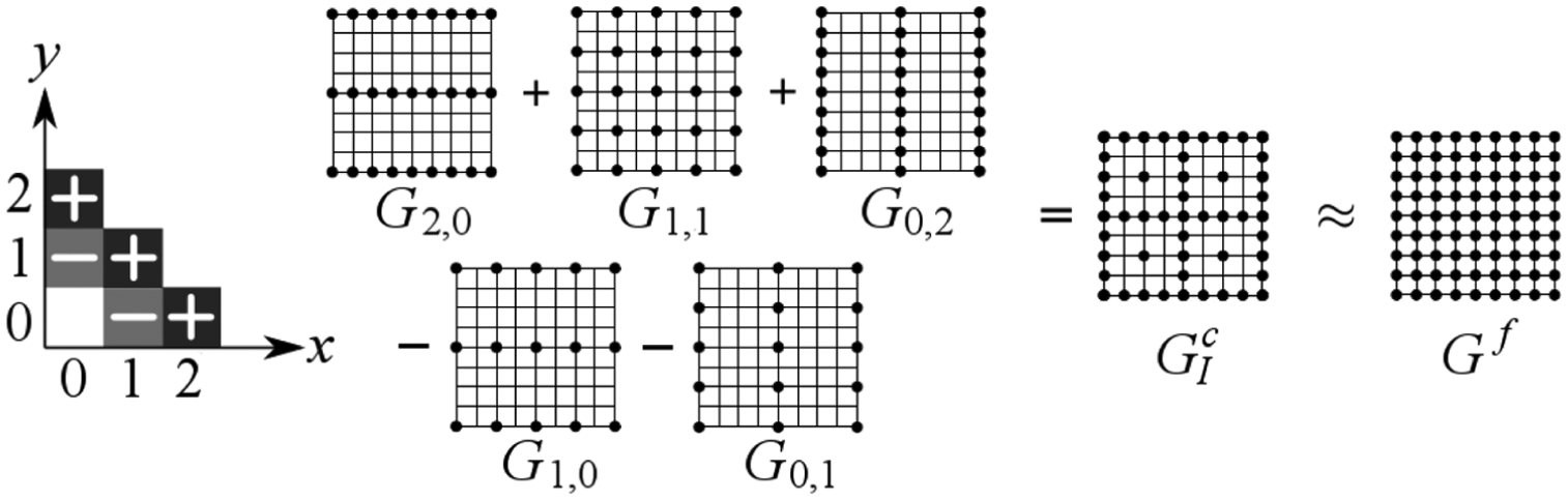
The SGCT (Griebel, 1992; Griebel et al., 1992) is a method of approximating the sparse grid solution which in turn approximates the full grid solution. Instead of solving the PDE on a full isotropic grid, it is solved on a set of small anisotropic regular grids referred to as sub-grids or component grids, represented by
Suppose that each sub-grid
where the
Note that level
Two levels of parallelism are achieved in the SGCT computation. Firstly, different sub-grids are computed in parallel. Secondly, each sub-grid,
In contrast to the full grid approach which consists of
3.3 FT sparse grid combination technique
An FT adaptation of the SGCT has been studied in Harding and Hegland (2013). In this article, we refer to this adaptation as FT-SGCT (FT SGCT). It is observed that the solution on even smaller sub-grids can be computed at little extra cost and that this added redundancy allows combinations with alternative coefficients to be computed. When a process failure affects one or more processes involved in the computation of one of the larger sub-grids, the entire sub-grid is discarded. In the event that some sub-grids have been discarded one must modify the combination coefficients such that a reasonable approximation is obtained using solutions computed on the remaining sub-grids. In 2-D, this involves finding
For the 2-D FT SGCT computations in this article, two extra layers (or diagonals) of sub-grid solutions
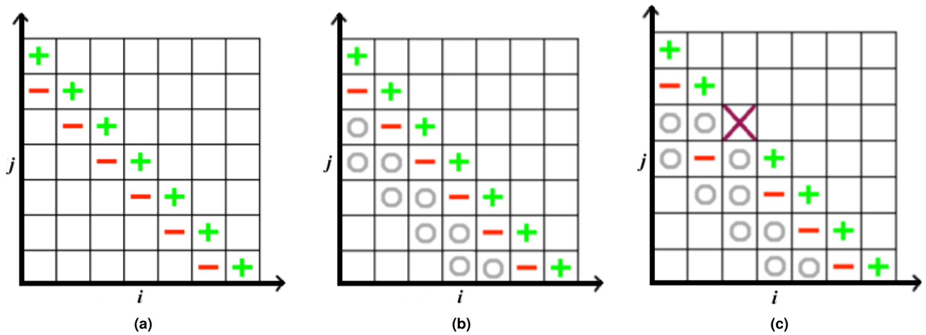
A depiction of the 2-D SGCT. “+,”“–,” and “o” on a sub-grid denotes the computed solution on that sub-grid is added, subtracted, and ignored, respectively, on the combined solution. “x” on a sub-grid denotes the solution on that sub-grid is lost and ignored in the combination. (a) Classical SGCT, (b) fault-tolerant SGCT with extra smaller sub-grids on two lower layers (marked with “o”) and without any loss of sub-grid solution, and (c) fault-tolerant SGCT in the event of a lost solution on sub-grid
3.4 SGCT algorithm overview and process organization
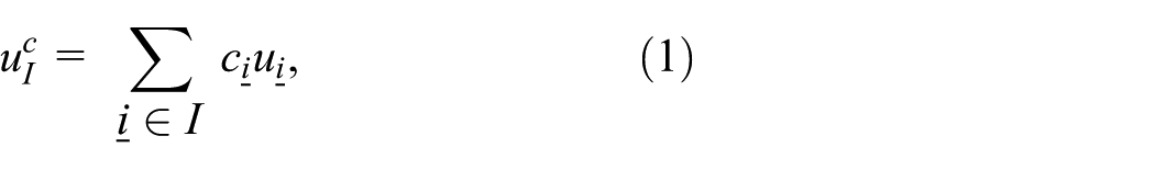
Referring to equation (1), each PDE instance whose solution is
In the scatter stage, each process in
Further details on the algorithm can be found in a companion article (Strazdins et al., 2015b). An improved version of this algorithm for performing interpolation on a sparse grid, rather than on a full grid, using a sparse grid data structure will be available in Strazdins et al. (2015a).
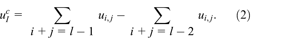
Our SGCT algorithm supports the so-called “truncated” combinations (Benk and Pfluger, 2012), where for the 2-D case, each component grid has
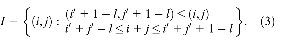
Extra layers are added to the set for the FT adaptation by changing the lower limit, for example,
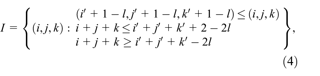
which may have additional sub-grids added in the FT adaptation.
In terms of load balancing, we used a simple strategy to balance the loads among the processes. Details are discussed and analyzed in Section 9.
A failure of computing nodes or application processes causes the loss of some processes on some grids
4 Experimental methodology
All experiments were conducted on the Raijin cluster managed by the National Computational Infrastructure (NCI) with the support of the Australian Government. Raijin has a total of 57,472 cores distributed across 3592 compute nodes each consisting of dual 8-core Intel Xeon (Sandy Bridge 2.6 GHz) processors (i.e. 16 cores) with Infiniband FDR interconnect, a total of 160 TBytes (approximately) of main memory, and 10 PBytes (approximately) of usable fast filesystem (NCI).
We used git revision
Faults were injected into the application by aborting single or multiple MPI processes at a time (with the exception of process 0 as it held critical data) by the system call
The integrated performance monitoring (IPM) profiler was used to report the total memory usage of the applications.
Approximation error was represented by the relative l1 error of combined field. It was computed by
5 General methodology for the SGCT integration
Our underlying SGCT algorithm is implemented in C++ (Strazdins et al., 2015b). Applications implemented either in C++ or other languages require an integration with it to exchange the
Algorithm 1 describes the main program, written in C++, calling into the application. A global communicator W is used to create a set of sub-grid communicators
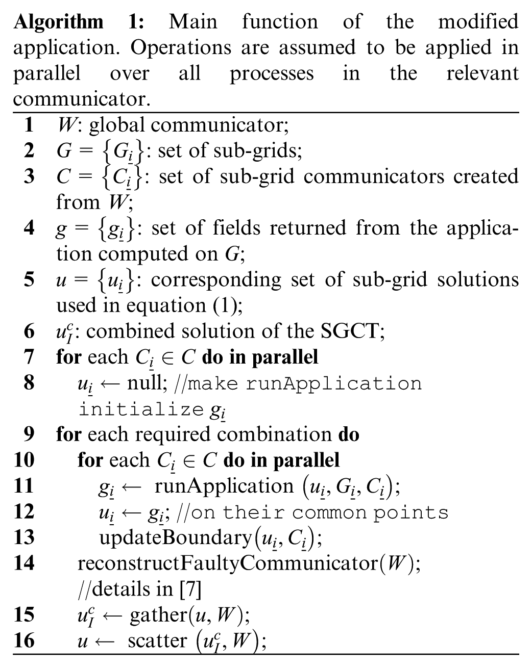
The set of sub-grid solutions
Process or node failures may happen after line 7 in Algorithm 1 once the program starts executing. In order to tolerate these failures, the faulty communicator is reconstructed (line 14, details are in Ali et al., 2014). Then the FT-SGCT is applied using the communicator W, with the combined solution
Multiple combinations over the simulation may also improve the accuracy of the combined solution. Additionally, it may cause less data loss in the presence of failures. Since it combines component solutions several times, the effect of failures may be restricted to the subsequent combination.
It is necessary to exchange
The main program uses the SGCT implementation to determine the parallel domain decomposition to be used by the application.
The main program creates a different directory for each application instance with a customized input parameter file containing the necessary values required for this instance.
MPI error handlers are attached to all MPI communicators and sub-communicators in the code. With a communicator or sub-communicator comm, the error handler function utilizes the
6 FT SGCT with the gyrokinetic plasma application
In this section, we discuss in detail the technique of applying the FT-SGCT to the gyrokinetic plasma application (GENE), including experimental evaluations. An overview of the application is presented in Section 6.1. Section 6.2 describes how the SGCT algorithm is integrated into the higher dimensional grids and includes a detailed discussion of parallelization over non-SGCT dimensions. The modifications required for the application of GENE are discussed in Section 6.3. Finally, an experimental evaluation of the FT-SGCT for GENE is presented in Section 6.4.
6.1 Application overview
The GENE (Görler et al., 2011; Jenko and the GENE development team, 2014) is a plasma micro-turbulence application code. It contains a multidimensional solver of gyrokinetic equations for a field comprised of ion and electron densities defined on a fixed grid in a five-dimensional (5-D) phase space
This field is one of the main outputs of GENE; from it, GENE computes gyroradius-scale fluctuations and transport coefficients.
The code base (Jenko and the GENE development team, 2014) is written in Fortran 90 and utilizes hybrid MPI/OpenMP parallelization. High scalability to 10K cores has been reported (Görler et al., 2011). Due to the relative smoothness of the solution, the SGCT has yielded good results in producing a relatively accurate solution on important problem sets (Kowitz et al., 2012).
Internally, GENE uses a complex precision array (
All processes in a running GENE instance read the same parameter file
For performing the “initial value” computation (Eriksson et al., 1996) of GENE, the main subroutine
6.2 Implementation of the SGCT algorithm for higher dimensional grids
The field of GENE, regarded as a field of real numbers, can be thought of an array with the following dimensionality:

The first element in D arises from the field being complex (note that the SGCT uses only additions and multiplications with real coefficients).
Our implementation performs the SGCT across such a field as follows. The dimensions for the SGCT must be a contiguous sub-vector of D. Any remaining lower dimensions of D can be dealt with by an extension to the algorithm to operate on blocks of
For example, to perform a 2-D combination on the
Our SGCT algorithm supports parallelization over arbitrary process grids in the SGCT dimensions. To support a parallelization to a total factor of
The implementation of this requires the careful construction of MPI communicators for each process sub-grid; the details of this are as follows.
Parallelization on non-SGCT dimensions changes the original block definition and their placement. With parallelization
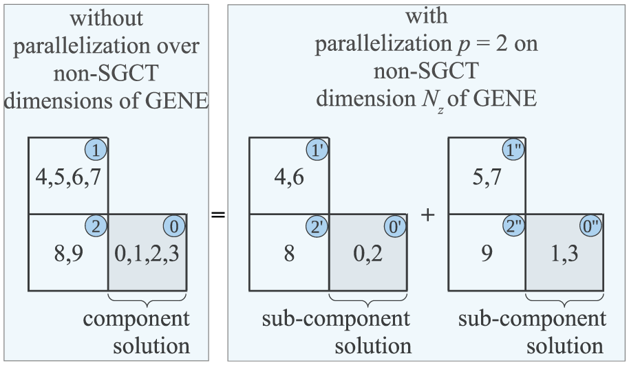
A demonstration of parallelization
6.3 Modifications to GENE for the SGCT
Some modifications to the GENE source were required to exchange
Referring to the main program of Algorithm 1, after copying common elements from
and then copy into
The main program uses the SGCT implementation to determine the parallel domain decomposition to be used by GENE. Furthermore, each GENE instance will have different global sizes for the dimensions used in the combination (e.g. for the 3-D SGCT, these might be
A standard tool is utilized for the interoperability between C and Fortran as an interface. We used the intrinsic module
The
One extra parameter is added to the
In the
Then,
6.4 Experimental results
In this section, the experimental setup, an analysis of the execution performance, and the memory consumption of both the FT-SGCT and equivalent full grid computations for GENE are presented. Following this, we discuss the approximation errors of the solutions computed with FT-SGCT for GENE.
6.4.1 Experimental setup
Experiments were conducted based on a problem from the GENE testsuite (
The selection of levels
6.4.2 Execution performance
Figure 4(a) gives execution performance of the 2-D FT-SGCT, 3-D FT-SGCT, and the equivalent full grid computations for GENE. It is observed that the 2-D FT-SGCT is
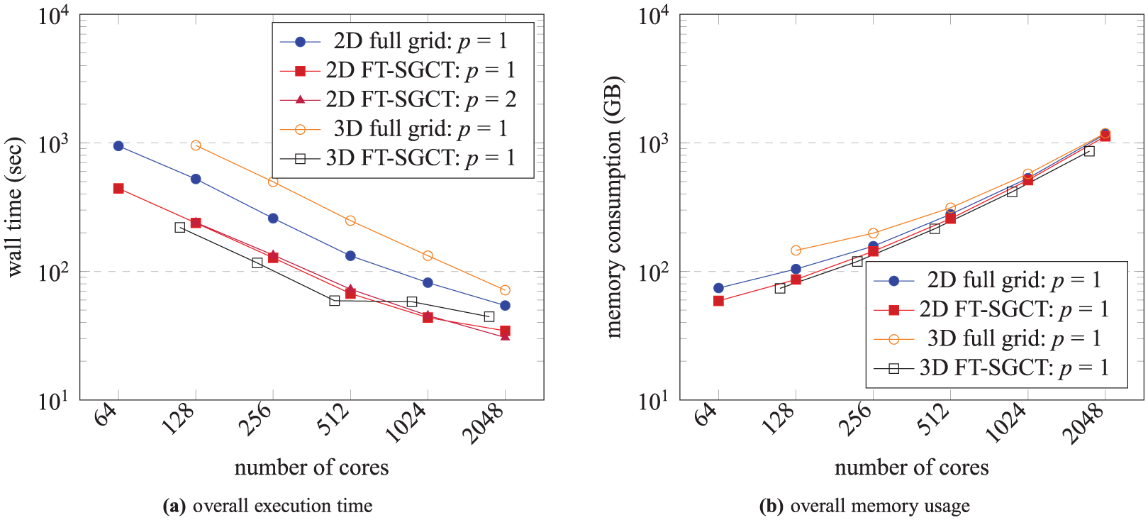
Overall execution time and memory usage of the 2-D FT-SGCT, 3-D FT-SGCT, and the equivalent full grid computation with a single combination when there is no fault throughout the computation for GENE. 2d_big_6 and 3d_big_6 inputs are used for the 2-D and 3-D FT-SGCT computations, respectively, which are different. Results shown are an average of two experiments; p represents parallelization on the non-SGCT dimension (
Figure 4(a) also provides evidence that our FT-SGCT implementation supports parallelization over non-SGCT dimensions for GENE. For the 2-D case, we choose a parallelization
Table 1 shows the overall performance of the 2-D FT-SGCT for the GENE application in isolation. It is observed that performing the combination is not costly. It should be noted however these times are for when the SGCT algorithm has been called before the application starts to exclude the Open MPI warm-up time. As explained by Strazdins et al. (2015a), the cost of the first call to the SGCT can be much greater, due to the fact that Open MPI is required to setup new connections between processes operating on separate sub-grids. For a detailed analysis and evaluation of the combination algorithm, see Strazdins et al. (2015a, 2015b).
Execution time breakdown of the 2-D FT-SGCT with
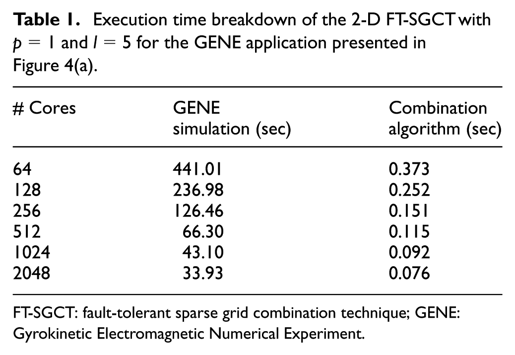
FT-SGCT: fault-tolerant sparse grid combination technique; GENE: Gyrokinetic Electromagnetic Numerical Experiment.
6.4.3 Memory usage
Figure 4(b) gives a comparison of memory usage of the 2-D and 3-D FT-SGCT with the equivalent full grid computation for GENE. It is observed that the memory requirement of the FT-SGCT is roughly the same as that of the equivalent full grid for the relatively small SGCT level used. A bigger improvement in memory usage would be expected for larger levels.
6.4.4 Approximation errors
Figure 5 shows the approximation errors of the 2-D and 3-D FT-SGCT with varying number of combinations and varying number of lost sub-grids for GENE. It is observed that the error is acceptably low for both the 2-D and 3-D cases. Moreover, multiple combinations clearly show advantages on faulty systems.
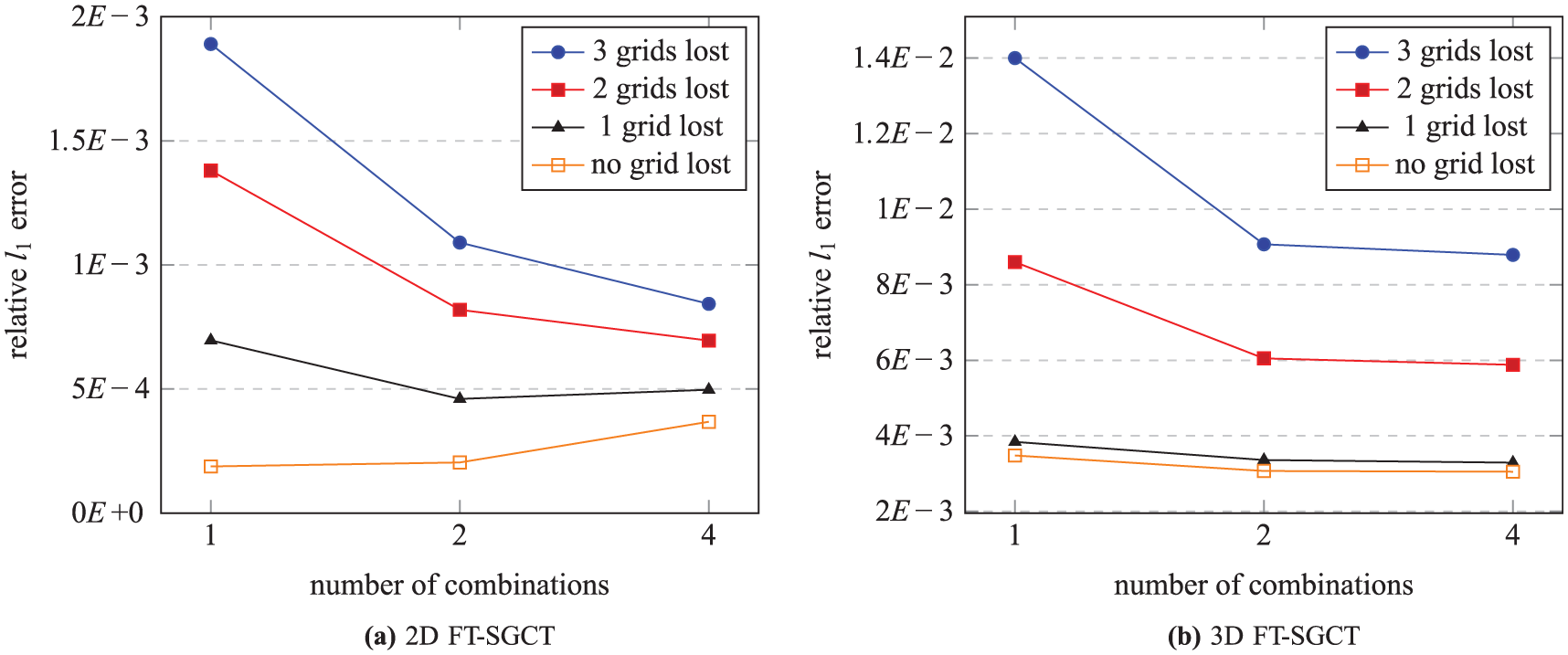
Approximation errors of the FT-SGCT for GENE. 2d_big_6 and 3d_big_6 inputs are used for the 2-D and 3-D FT-SGCT computations, respectively, which are different. Results shown are an average of a number of experiments for the loss of 1 component grid, 2component grids, and 3 component grids such that the occurrence of faults maintains an uniform distribution over all computing nodes. In order to do so, we injected 62% of the failures on the first diagonal (on larger grids, except grid 0), 25% on the second diagonal, 10% on the third diagonal, and 3% on the fourth diagonal (on smaller grids) for the 2-D FT-SGCT. For the 3-D FT-SGCT, these are 72%, 22%, 55, and 1%, respectively. However, for non-failure case, only one experiment is done.
Furthermore, Figure 6 shows some plots of the combined and equivalent full grid solution densities in the absence or presence of faults for GENE. It demonstrates how much a field deteriorates due to approximation error. It is observed that even with
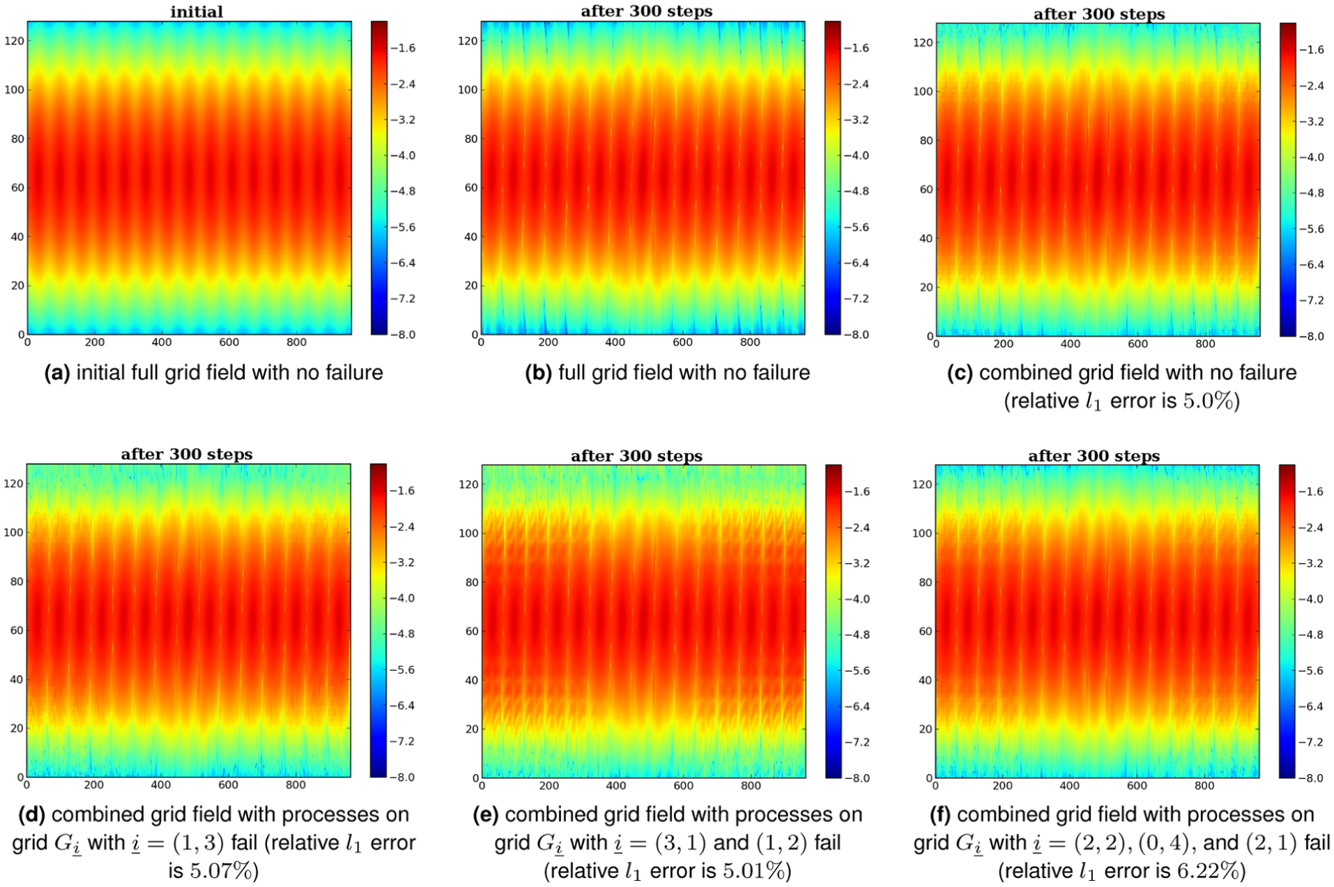
Comparison of the 2-D full grid and level 5 combined grid solutions with
7 FT SGCT with the LBM application
In this section, we discuss the Taxila LBM application, the modifications needed on Taxila LBM to apply the SGCT, and the experimental evaluation of the FT-SGCT for Taxila LBM.
7.1 Application overview
The LBM is used to solve the discrete Boltzmann equation. The equation is used to evolve the general form of a distribution function for a lattice:
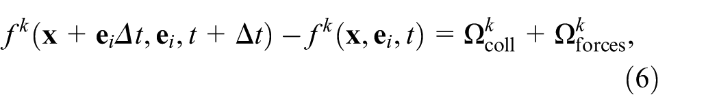
where
The popularity of LBM for the pore–scale simulation is increasing due to its capability of including complex geometries without putting more effort. Other benefits include multiple relaxation times, increased isotropy, improved accuracy, and physical fidelity of the method. The explicit type of algorithm and comparatively huge local task provide a benefit of achieving high computational efficiency (Coon et al., 2014).
Taxila LBM (Coon et al., 2014; Porter et al., 2012) is an open-source software framework of the LBM for simulation of flow in porous and geometrically complex media. It is based upon the Shan–Chen model (Shan and Chen, 1993). This framework provides some excellent features: (1) it is shown that the implementation is scalable to tens of thousands of cores on Jaguar/Titan; (2) its Fortran 90 based PETSc (Balay et al., 2014) modular implementation is easily extendable; (3) it provides the flexibility of solving D2Q9 (2-D, 9 lattice velocities), D3Q19 (3-D, 19 lattice velocities), and other mesh dependencies, on the 2-D or 3-D grids; (4) it supports arbitrary, heterogeneous boundary conditions, and multiple mineral/wall materials; (5) it can operate on multiphase systems with different phase viscosities and/or molecular masses; and (6) it provides flexibility to include higher order derivatives or multiple relaxation times to improve the stability at large viscosity ratios.
In this work, we chose an example application available under
By default, the bubble test provides a distribution function field as output. It is also possible to extract either the density, total velocity, total density, or pressure fields. In our experiment, we choose the density field as output.
7.2 Modifications to Taxila LBM for the SGCT
Some modifications to the Taxila LBM source were required to exchange
An interface is created to communicate between C++ and PETSc (Fortran 90 code). A standard tool is used for the interoperability between C and Fortran. A C wrapper of the C++ code is used to hide the C++ code from the implementation. An intrinsic module ISO_C_BINDING and the language-binding-spec BIND is used for the interoperability.
In the original Taxila LBM implementation, the bubble format is fixed. We made it adaptive based on the number of grid points in each dimension. For each grid, we define the suspending bubble as a square/rectangle of length of one-half of the number of grid points in each dimension and placed it at the center of the corresponding grid.
The default global communicators in the
The original Taxila LBM requires a single parameter file
Since density is the field of interest to which the SGCT is applied, we extract the local rho field after finishing the execution of the
Process or node failures are handled by the similar way as it is handled for the GENE application.
In order to facilitate multiple combinations,
7.3 Experimental results
In this section, the experimental setup, an analysis of the execution performance, and memory consumption of both the FT-SGCT and equivalent full grid computations for Taxila LBM are presented. Following this, we discuss the approximation errors of the solutions computed with the FT-SGCT for Taxila LBM.
7.3.1 Experimental setup
Experiments were conducted with the parameters in
Parameters in
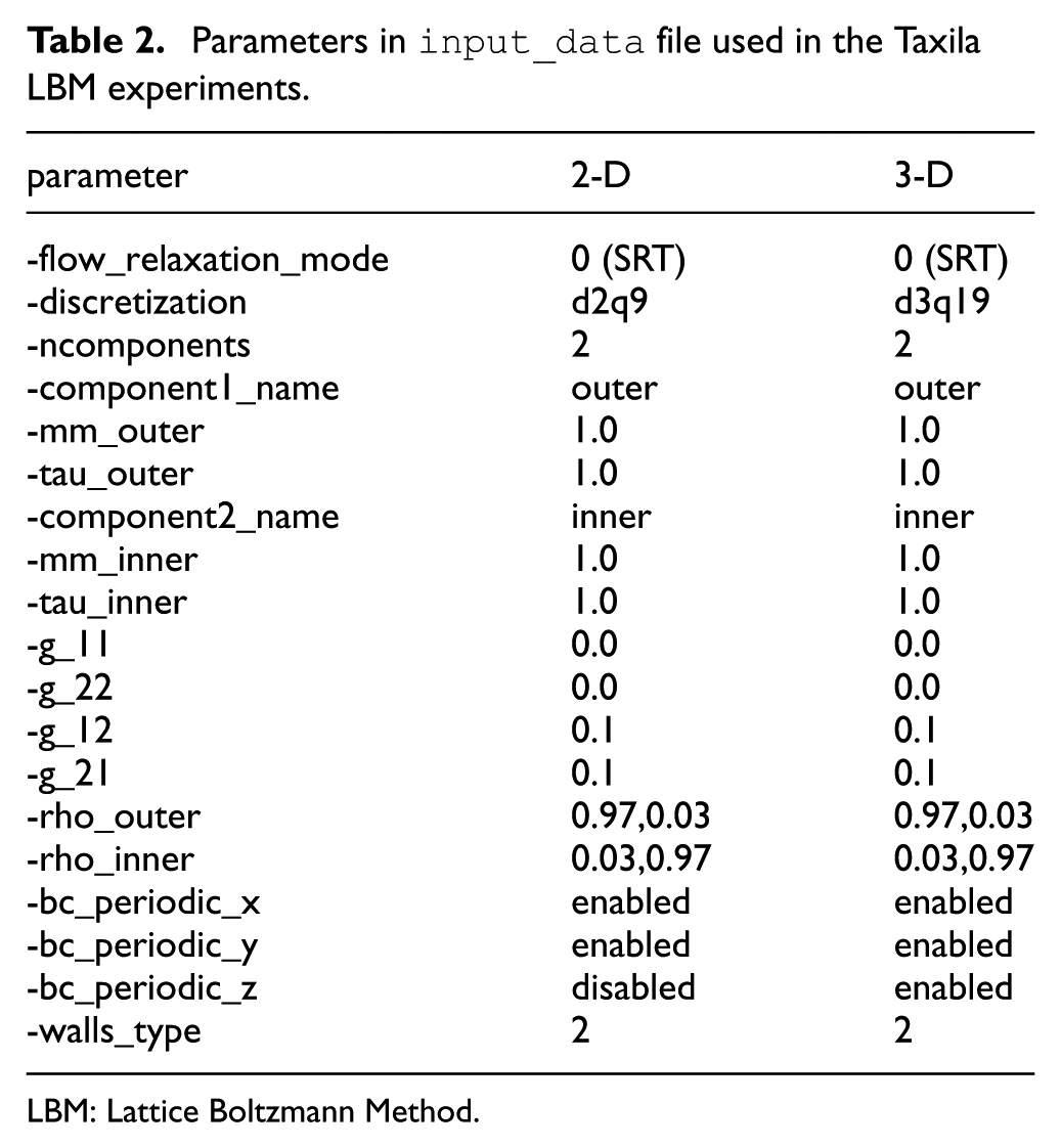
LBM: Lattice Boltzmann Method.
7.3.2 Execution performance
Figure 7(a) shows the execution performance of the 2-D FT-SGCT, 3-D FT-SGCT, and the equivalent full grid computations for Taxila LBM. It is observed that the 2-D FT-SGCT is
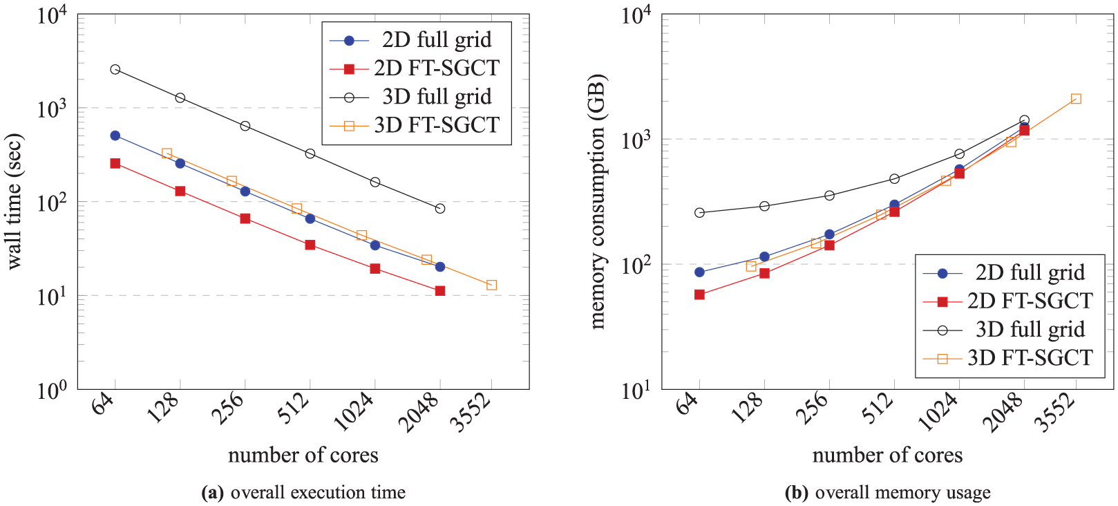
Overall execution time and memory usage of the 2-D FT-SGCT, 3-D FT-SGCT, and the equivalent full grid computation with a single combination when there is no fault throughout the computation for the Taxila LBM application. 2-D FT-SGCT computes
Table 3 shows the overall performance of the 2-D FT-SGCT for the Taxila LBM application in isolation. It is observed that performing the combination is again of little relative cost. It should be noted however these times are again for when the SGCT algorithm has been called before the application starts to exclude the Open MPI warm-up time.
Execution time breakdown of the 2-D FT-SGCT with
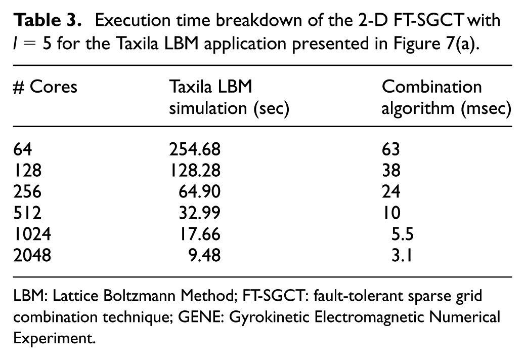
LBM: Lattice Boltzmann Method; FT-SGCT: fault-tolerant sparse grid combination technique; GENE: Gyrokinetic Electromagnetic Numerical Experiment.
7.3.3 Memory usage
Figure 7(b) shows the amount of memory usage of the 2-D FT-SGCT, 3-D FT-SGCT, and the equivalent full grid computations for Taxila LBM. It is observed that the memory requirement of the FT-SGCT is roughly the same as that of the equivalent full grid for the relatively small SGCT level used. A bigger improvement in memory usage would be expected for larger levels.
7.3.4 Approximation errors
The computed relative l1 approximation errors of the 2-D and 3-D FT-SGCT for Taxila LBM are
Furthermore, Figure 8 shows some plots of the combined and equivalent full grid solution densities in the absence or presence of faults for Taxila LBM. It demonstrates how much a field deteriorates in the presence of faults. It is observed that even with
Comparison of the full grid and level 5 combined grid solutions with
8 FT SGCT with the SFI application
In this section, we discuss the SFI application, the modifications needed on SFI to apply the SGCT, and the experimental evaluation of the FT-SGCT for SFI.
8.1 Application overview
The Bratu problem in 3-D coordinates is defined by the following equation:

where
In this work, we chose an application solving the Bratu problem for the modeling of SFI (or combustion) with
This targeted application is not as complex compared to the previous applications. However, evaluation of this application will provide us a general idea about the evaluation of large complex applications modeling SFI.
8.2 Modifications to SFI for the SGCT
Some modifications to the SFI source were required to exchange
The PETSc code base of the 2-D SFI is in Fortran 90. A standard tool is used for the interface between C and Fortran. A C wrapper of the C++ code is used to hide the C++ code from the implementation. An intrinsic module
The default global communicators in the
The
Process or node failures are handled in the similar way as it is handled for the GENE application.
Multiple combinations are achieved by passing
8.3 Experimental results
In this section, the experimental setup, an analysis of the execution performance, and memory consumption of both the FT-SGCT and equivalent full grid computations for SFI are presented. Following this, we discuss the approximation errors of the solutions computed with the FT-SGCT for SFI.
8.3.1 Experimental setup
Experiments were conducted with Bratu parameter
8.3.2 Execution performance
Figure 9(a) shows the execution performance of the 2-D FT-SGCT, 3-D FT-SGCT, and the equivalent full grid computations for SFI. It is observed that the 2-D FT-SGCT is
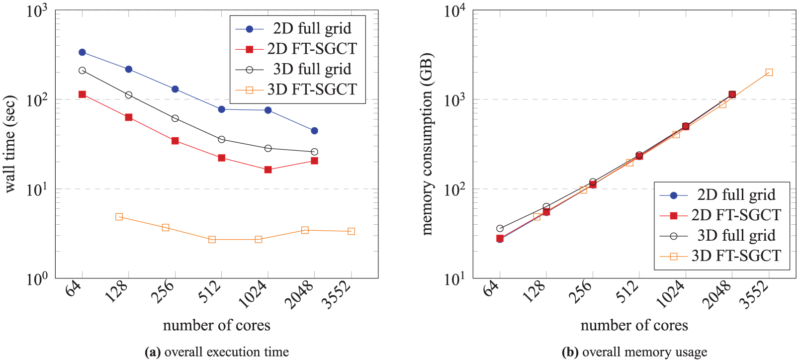
Overall execution time and memory usage of the 2-D FT-SGCT, 3-D FT-SGCT, and the equivalent full grid computation with a single combination when there is no fault throughout the computation for the SFI application. 2-D FT-SGCT computes
Table 4 shows the overall performance of the 2-D FT-SGCT for the SFI application in isolation. It is observed that the overhead of performing the combination is very low. It should be noted however these times are for when the SGCT algorithm has been called before the application starts to exclude the Open MPI warm-up time.
Execution time breakdown of the 2-D FT-SGCT with
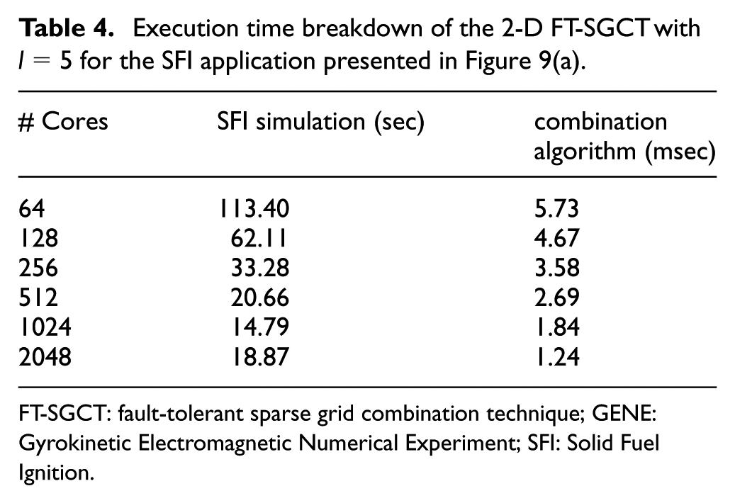
FT-SGCT: fault-tolerant sparse grid combination technique; GENE: Gyrokinetic Electromagnetic Numerical Experiment; SFI: Solid Fuel Ignition.
8.3.3 Memory usage
Figure 9(b) shows the amount of memory usage of the 2-D FT-SGCT, 3-D FT-SGCT, and the equivalent full grid computations for SFI. It is observed that the memory requirement of the FT-SGCT is roughly the same as that of the equivalent full grid for the relatively small SGCT level used. A bigger improvement in memory usage would be expected for larger levels.
8.3.4 Approximation errors
The computed relative l1 approximation errors of the 2-D and 3-D FT-SGCT for SFI are
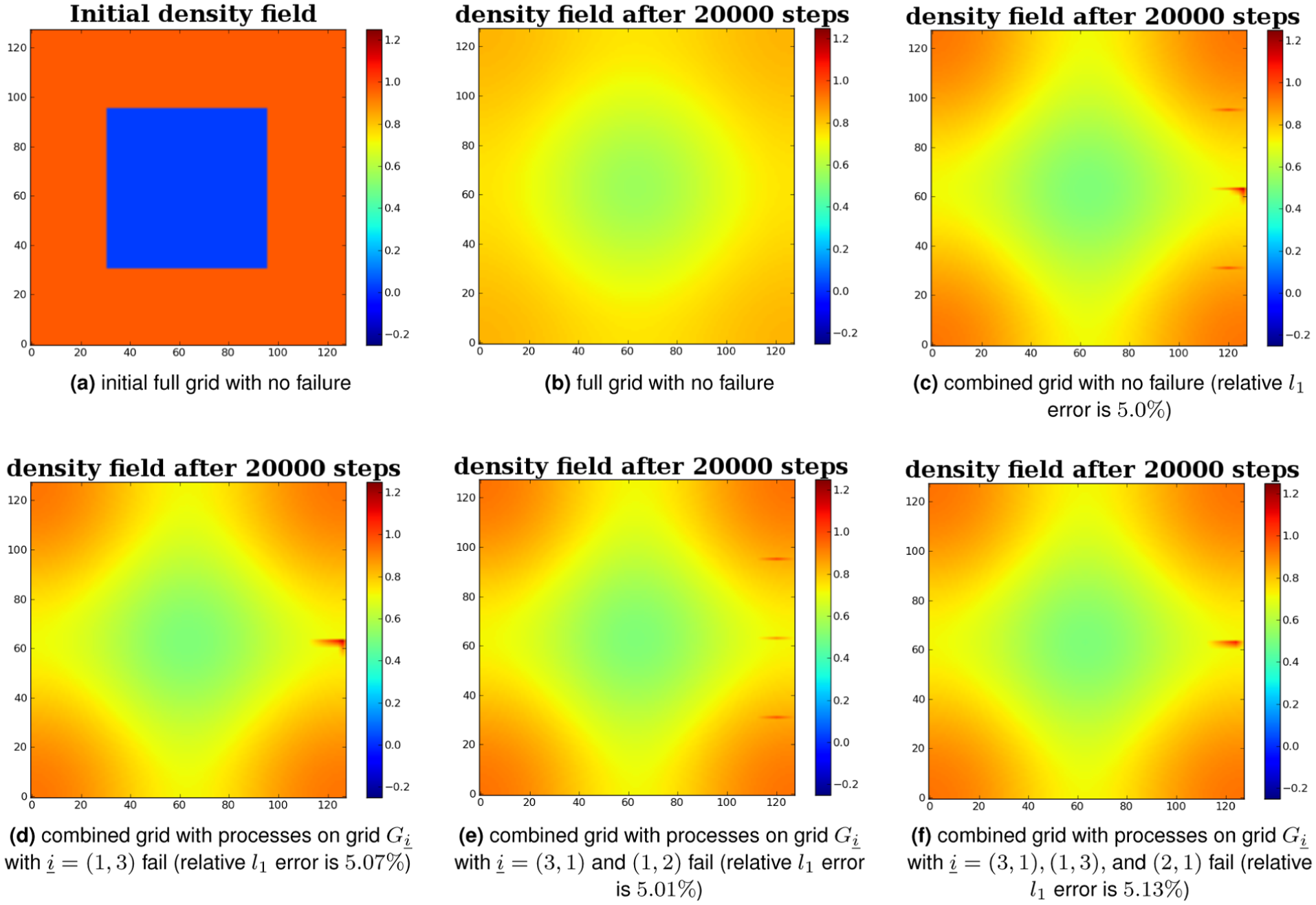
Furthermore, Figure 10 shows some plots of the combined and equivalent full grid solution densities in the absence or presence of faults for SFI. It demonstrates how much a field deteriorates in the presence of faults. It is observed that with
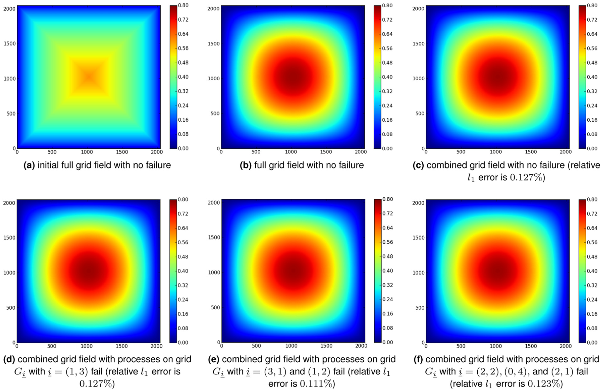
Comparison of the full grid and level 5 combined grid solutions with
9 Load balancing
A simple strategy is used to balance the load among the processes to execute applications using SGCT. The same number
An analysis of load balancing is carried out based on this balancing strategy. The TAU profiling tool (Shende and Malony, 2006) is used to generate the load balancing results. It is observed from Figure 11 that the first order approximation of loads to each process sufficiently balances loads among the MPI processes (ranks) for the 2-D FT-SGCT computing GENE application. However, it can be seen that the second sub-grid is computed fastest, and the first and fourth sub-grids are slowest.
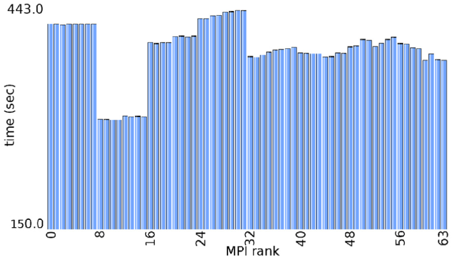
Analysis of the TAU-generated load balancing of the 2-D FT-SGCT computing the GENE application on level 5 with a single combination.
The GENE application is observed to be very sensitive to the number of processes allocated to each of its five dimensions (excluding species). In our current implementation, we set processes only for the two or three dimensions (for the 2-D and 3-D FT-SGCT, respectively), and the remaining are set to 1. The process grid for the second sub-grid properly distributes the processes across all the dimensions, so it is computed fastest.
The load balancing of the 3-D version of this application and of both the 2-D and 3-D versions of other applications shows similar characteristics to this. Thus, those results are not presented here separately.
10 Failure recovery overheads
In this section, we analyze the recovery overheads of the FT-SGCT using ULFM with that of the SGCT implementation using Checkpoint/Restart (Hursey et al., 2007) (represented by CR-SGCT), recovery overheads of the FT-SGCT in terms of computing extra unknowns, and repeated failure recovery overheads.
10.1 Recovery overheads for shorter computations
Figure 12(a) shows the component timings that are used to estimate the recovery overheads of the two approaches. The first component timing is related to the implementation of the FT-SGCT, which uses ULFM MPI and the algorithm-based recovery (in terms of applying alternate combination formula) on the SGCT to recover from failures. The second component timing is related to the implementation of the CR-SGCT, which uses a Checkpoint/Restart-based recovery on the SGCT to recover from failures. The components are generated using 2d_big_6 input of GENE and will be used for measuring the overheads of both the shorter and longer computations. Component timings for the other two applications (Taxila LBM and SFI) are almost the same as these. So, they are not presented separately.
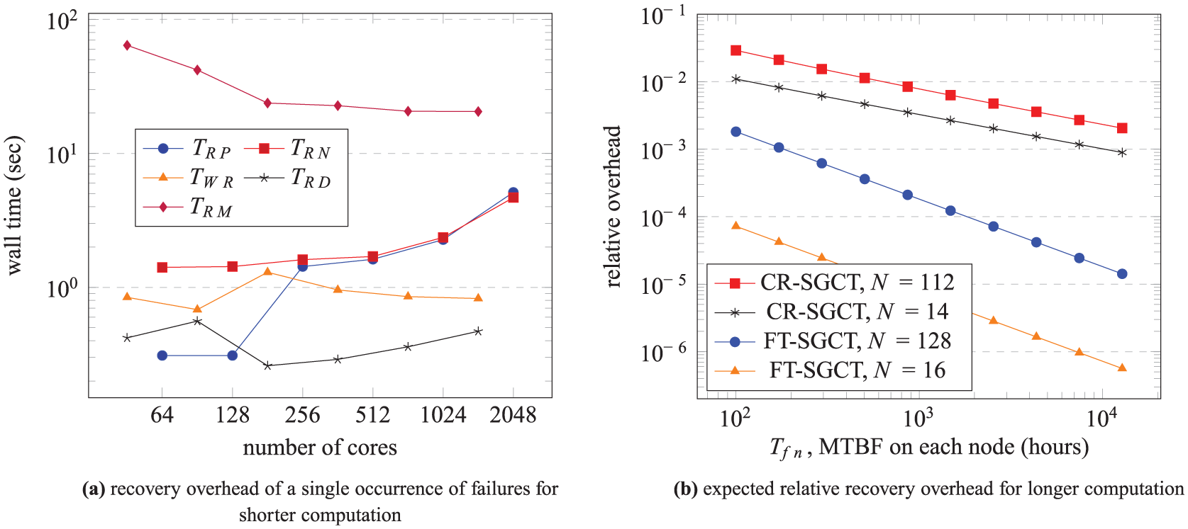
Recovery overheads for shorter and longer computations for GENE. Results shown are an average of two experiments for 2d_big_6 input applied to the 2-D SGCT. The notations used in the legends are from Section 10. GENE: Gyrokinetic Electromagnetic Numerical Experiment; FT-SGCT: fault-tolerant sparse grid combination technique.
The notations in this figure are as follows.

where
– t1 is the system time of running the CR-SGCT for 50 timesteps with global checkpoint write at the end (no checkpoint read),
– t2 is the system time of running the CR-SGCT for 50 timesteps after initializing from checkpoint (written on previous step) and no global checkpoint write, and
– t3 is the system time of running the CR-SGCT for 100 timesteps with global checkpoint write at the end (no checkpoint read).
Based on the process times, it is possible to estimate the recovery overheads for the shorter computations (since shorter computation saves CPU hours). The overheads of the FT-SGCT of a one-off process and node failures are
It should be noted that we would expect that
10.2 Recovery time analysis for longer computations
Using results gathered so far, we will estimate the overhead of our implementation for longer computations and different frequencies of faults. We will compare this estimate with the time of the CR-SGCT taking into account the overhead generated by having to backtrack to the previous checkpoint when failures occur. It is assumed that the occurrence of faults is independent and identically distributed on each compute node. Further, it is assumed that faults are exponentially distributed and therefore the failure rate is constant. The other variables we use are as follows:
N is the number of nodes used in the computation.
C is the number of combinations throughout the computation.
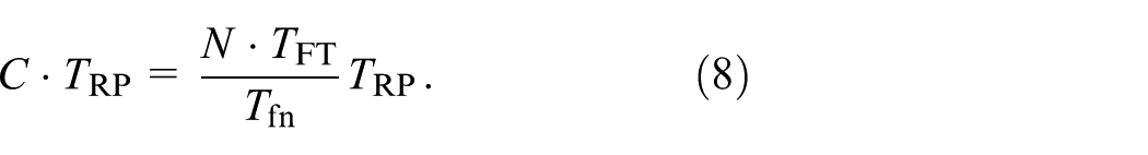
Experimental results presented in Figures 4(a) and 12(a) allow us to estimate
One sees that this is inversely proportional to the MTBF per node. Note that the occurrence of faults obviously affects the error of the SGCT. The estimation of this error, however, is more involved.
We will compare the algorithm-based recovery overheads of the FT-SGCT with the typical overhead of the Checkpoint/Restart applied to the SGCT computation. Here we define some additional values of interest:
Experimental results summarized in Figures 4(a) and 12(a) allow us to estimate
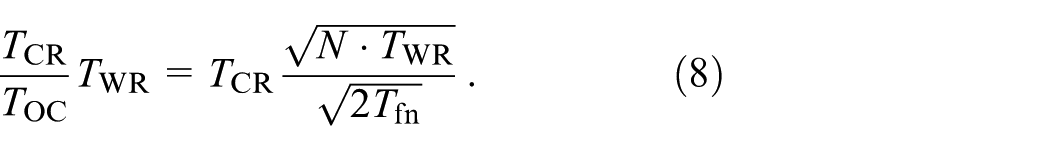
The total overhead for Checkpoint/Restart consists of two components. The first is the writing of checkpoints, which throughout the computation is as follows:
Additionally, for each failure, MPI must be restarted, a checkpoint read, and recomputation done up to the point at which the failure occurred. This overhead is the restart time plus the typical recomputation time multiplied by the expected number of faults, that is:
Adding the two together the total Checkpoint/Restart overhead is:
Note that this overhead obviously extends the execution time of the application thus exposing it to more faults and that the same applies for the overhead with algorithm-based recovery. One may, however, divide the application execution time out of both overheads and instead compare the overheads relative to the application execution times. We are particularly interested in how the two compare as the time between failures varies. The change in relative overheads with respect to
10.3 Overhead due to computing extra grid points
Some extra sub-grid computations are needed in the SGCT to achieve an algorithm-based fault resiliency called FT-SGCT. The amount of redundancy determines the accuracy of the combined solution in the event of a number of sub-grid losses at a time. It could be selected based on the reliability of the system running the SGCT application. The more failure-prone the system is, the more the redundant sub-grid computation is required to achieve the combined solution with a reasonable approximation error.
The number of grid points on each sub-grid of a layer/plane is half that of its upper (higher) layer/plane. With the current load-balancing strategy, this principle also applies to the number of cores, if single-threaded MPI processes are used. For the 2-D FT-SGCT, the overhead of computing extra grid points relative to computing the total grid points in the SGCT is defined using the following equation:
where
where
The relative overhead of our 2-D FT-SGCT implementation (with level
The minimum, maximum, and the implementation-specific relative overheads of the 2-D and 3-D FT-SGCT for various levels are shown in Figure 13. It is observed that the maximum relative overhead of the 3-D FT-SGCT is more than 2× lower compared to the 2-D case. This indicates that the relative overhead will be significantly reduced if combination is performed on higher dimensions, rather than on lower dimensions.
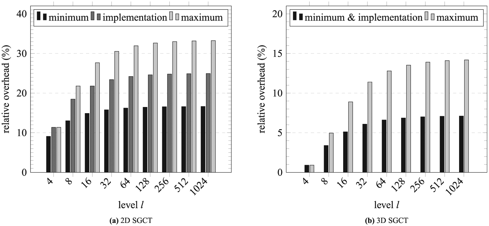
Relative overhead required in the SGCT to achieve an ABFT. It is calculated by dividing the total grid points in the SGCT out of extra grid points computed in the FT-SGCT. For the 2-D case, minimum, implementation, and maximum are calculated with
10.4 Repeated failure recovery overheads
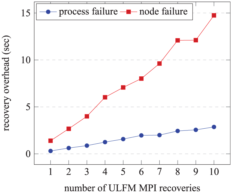
Repeated ULFM MPI failure recovery overheads of the 2-D FT-SGCT with
11 Conclusions
In this article, we have presented an overview of a general parallel SGCT combination algorithm and its associated load-balancing strategy. The algorithm can be applied over several of the dimensions of a multidimensional field of a PDE time-evolving application. It also easily supports parallelization in the non-SGCT dimensions. Thus, it is capable of supporting extremely large-scale applications.
We have shown how, using a general methodology, it can be integrated into three existing, complex real-world applications (GENE, Taxila LBM, and SFI) with minimal changes to the source code. The software engineering effort required to integrate the SGCT into the application was acceptable. Even if the application has the complication of nontrivial boundary conditions, which needs to be applied for the SGCT, it is likely the application itself will provide the required code, as was the case for GENE. Not only can the application benefit from the efficiency–accuracy trade-offs of the SGCT, for a relatively small amount of extra effort, it can also be made FT.
For relatively large fields, the large core count overhead of the combination was of the order of1–100 msec, easily acceptable compared with the current and near future MTBFs, and negligible compared with typical simulation execution times. We have also shown that the Taxila LBM and SFI applications are suitable applications for the SGCT. The latter is especially so with the very low error rates giving the SGCT a very favourable accuracy–performance trade-off.
Using a recent release to the ULFM MPI, our resulting implementation is robust to surviving multiple failures and recoveries, tested up to 2048 cores. We have shown that the 2-D, and especially the 3-D, SGCT have significant computational efficiencies compared with the traditional full grid simulation while having acceptable losses in accuracy. We did find however that the “smoothness” of the dimensions of the field chosen for the SGCT were important in this respect. In the case of multiple failures, multiple combinations can be used to reduce the error.
We have shown that the SGCT in conjunction with ULFM MPI can be used to recover a complex application from both process and node failures. Compared with the built-in checkpoint infrastructure in the GENE application and job restart from the checkpoint, our approach has
We have analyzed that in our experiments only a 14.29% and 0.91% redundancies are required to make the classical SGCT fault-tolerant for the 2-D and 3-D cases, respectively. An increase in the number of sub-grids leads only to a very slow increase of the required redundancies.
We expect that our SGCT-based ABFT technique will show significant advantages on current and future platforms beyond the ones we had access to for this article. This includes both much larger systems where checkpointing overheads become prohibitive, and systems whose components are less reliable than supercomputer nodes, for example, very cheap processors operated at minimal voltage in order to save power.
Future work includes applying our methodology to other complex PDE simulations suitable to the sparse grid technique.
Footnotes
Acknowledgements
The authors thank Christoph Kowitz of Technische Universität München for providing a distribution of GENE and for advice on the application. The authors also thank Ethan Coon of Los Alamos National Laboratory for providing a distribution of Taxila LBM and for a valuable discussion on the application. Moreover, the authors thank their colleague Jay Larson for valuable advice and support. We are grateful to Fujitsu Laboratories of Europe for providing funding as the collaborative partner in this project, and for giving the opportunity to two authors as the summer research intern in the laboratories. We thank the National Computational Infrastructure (NCI), supported by the Australian Government, for the use of the Raijin cluster.
Declaration of Conflicting Interests
The author(s) declared the following potential conflicts of interest with respect to the research, authorship, and/or publication of this article. Alistair P Rendell and Jay W Larson from Australian National University.
Funding
The author(s) disclosed receipt of the following financial support for the research, authorship, and/or publication of this article: This research was supported under the Australian Research Council’s Linkage Projects funding scheme (project number LP110200410).
Author biographies
Md Mohsin Ali recently submitted a PhD thesis in the Research School of Computer Science at The Australian National University (ANU). He came to Australia from Bangladesh in 2012. He has done his masters from Canada and undergraduate from Bangladesh both majoring in computer science. His research interests include high-performance computing, algorithms, mobile computing, and computer networks.
Peter E Strazdins received his PhD in computer science from ANU in September 1990. Since 1990, he has been with the Department of Computer Science at ANU and was a member of the ANU-Fujitsu CAP Parallel Computing Project over the years 1990–2002, being Research Leader over 1999–2002. He is an associate professor at the Research School of Computer Science at ANU, where he was Associate Director (Education) over the years 2009–2013. His research interests include parallel algorithms and libraries, large-scale simulations on supercomputers, virtualization and resilience for HPC, and computer simulation, modelling, and performance analysis.
Brendan Harding completed a Bachelor of Philosophy with first class honours in mathematics at ANU in 2010 and recently submitted a PhD thesis at the Mathematical Sciences Institute. His research interests include sparse grids, high-performance computing and fractal geometry.
Markus Hegland received his PhD with Silver Medal in mathematics from the ETH, Zurich, Switzerland, in 1988. He was one of the inaugural research fellows at the newly formed Interdisciplinary Project Center for Supercomputing for 3 years. He came to ANU in 1992 on a 1-year stint in supercomputing after which he was supposed to continue at ETH. However, after a year his ANU contract was extended by 1 year and he resigned from ETH to stay at the ANU until now. Except for a short break of 7 years in computer science he has been a member of the MSI where he currently holds a professorial position. He has been awarded a Senior Hans Fischer Fellowship at the IAS of the Technical University of Munich from 2011–2013. He is still a member of the IAS Focus Group in High Performance Computing in computer science. He has been attracted to problems which appear to be computationally intractable due to the curse of dimensionality, ill-posedness, and dependency in parallel computing.