Fine-grained floating-point precision analysis

Abstract

Floating-point computation is ubiquitous in high-performance scientific computing, but rounding error can compromise the results of extended calculations, especially at large scales. In this paper, we present new techniques that use binary instrumentation and modification to do fine-grained floating-point precision analysis, simulating any level of precision less than or equal to the precision of the original program. These techniques have an average of 40–70% lower overhead and provide more fine-grained insights into a program’s sensitivity than previous mixed-precision analyses. We also present a novel histogram-based visualization of a program’s floating-point precision sensitivity, as well as an incremental search technique that allows developers to incrementally trade off analysis time for detail, including the ability to restart analyses from where they left off. We present results from several case studies and experiments that show the efficacy of these techniques. Using our tool and its novel visualization, application developers can more quickly determine for specific data sets whether their application could be run using fewer double precision variables, saving both time and memory space.

Keywords

floating-point binary instrumentation program analysis precision sensitivity

1 Introduction

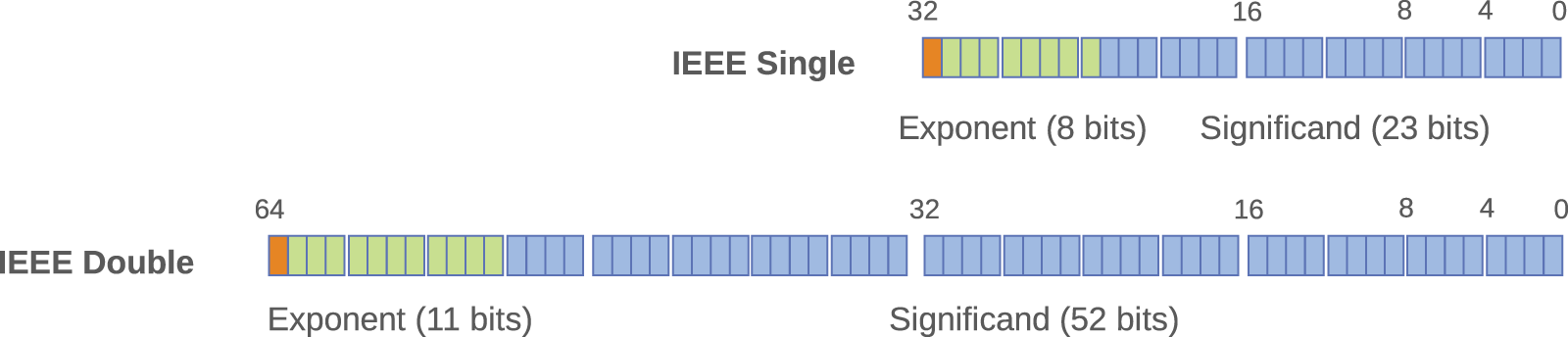
“Floating-point” is a method of representing real numbers in a finite binary format. It stores a number in a fixed-width field with three segments: (1) a sign bit (b); (2) an exponent field (e); and (3) a significand (or mantissa) (s). The stored value is $(- 1)^{b} \cdot s \cdot 2^{e}$ . Floating-point was first used in computers in the early 1940s, and was standardized by the IEEE in 1985, with the latest revision approved in 2008 (IEEE, 2008). The IEEE standard provides for different levels of precision by varying the field width, with the most common widths being 32 bits (“single” precision) and 64 bits (“double” precision). Figure 1 graphically represents these formats.

Figure 1.

IEEE standard formats.

Double-precision arithmetic results in more accurate computations, but with the costs of reduced parallelization, slower performance, and higher memory bandwidth and storage requirements. The main cost is the higher memory bandwidth and storage requirement, which are twice that of single precision. Another cost is the reduced opportunity for parallelization, such as on the x86 architecture, where packed 128-bit XMM registers can only hold and operate on two double-precision numbers simultaneously compared to four numbers with single precision. Finally, some architectures even impose a higher cycle count (and thus also energy cost) for each arithmetic operation in double precision. In practice, it has been reported that single-precision calculations can be 2.5 times faster than corresponding double-precision calculations, because of the various factors described above (Göddeke and Strzodka, 2011).

As high-performance computing continues to scale, these concerns will become increasingly important (Dongarra et al., 2011). Thus, application developers have powerful incentives to use a lower precision wherever possible without compromising overall accuracy. In addition, long-running computations may exhibit numerical accuracy issues not seen at smaller scales (He and Ding, 2001), providing even more impetus for an analysis solution that accounts for these runtime effects. Unfortunately, the numerical accuracy degradation of switching to single precision can be fatal, and many developers choose the “safe option” of sticking with double precision throughout their program.

In previous work, we presented techniques for performing automated mixed-precision analysis and configuration (Lam et al., 2013). Those mixed-precision techniques have proven useful, but sometimes the single-versus-double precision dichotomy is too coarse. It would be useful for a developer to be able to explore at a finer granularity how sensitive the various parts of a program are to changes in the floating-point precision level. In this paper, we describe our techniques for general precision-level analysis, based on binary modification for reduced precision. We also describe our implementation of these techniques in a generalized floating-point analysis framework. These techniques have an average of 40–70% lower overhead and provide more fine-grained insights into a program’s sensitivity than previous mixed-precision analyses.

The rest of the paper is arranged as follows. First, we describe our approach and implementation in Section 2. Second, we relate our evaluation and results in Section 3. Finally, we briefly enumerate related work in Section 4.

2 Our approach

We introduce a system for analyzing an application’s precision requirements. Our technique builds a version of a target program where every instruction can be executed at any level of precision lower than the original precision (i.e.“reduced” precision). Our techniques are implemented in the Configurable Runtime Analysis for Floating-Point Tuning (CRAFT) framework, a freely available software library for building floating-point binary analysis tools (see http://sourceforge.net/projects/crafthpc/). CRAFT is built on the Dyninst binary instrumentation framework (Buck and Hollingsworth, 2000) and provides additional support for analyzing and instrumenting floating-point programs. The framework can analyze any x86_64 program regardless of the source language (although the analysis is more useful if the program was compiled with debug symbols).

Using an automated search, we detect the smallest level of precision that any particular instruction can run with and still pass a user-provided verification routine, assuming that the rest of the program runs in its original precision. The results of the automated search give an indication of the precision level requirement of that instruction, which can be generalized to larger structures by taking the maximal value across all their children.

2.1 Automatic search

Using a binary truncation technique (described in detail in later sections), we developed a branch-and-bound automatic search routine that determines the general precision sensitivity of an increasingly granular set of program components. The technique uses a breadth-first search, similar to the mixed-precision search described in previous work (Lam et al., 2013). It first determines (using a single binary search on the range 0–52) the precision level required at the program level. Then, it explores the program’s subprogram components by doing binary precision searches on each subcomponent. For each binary search, the results of all floating-point instructions in the component are truncated to the precision being tested, while all other components remain at their original precision. The search gradually descends through various types of subcomponents: beginning with modules, it continues down through functions and basic blocks until it reaches individual instructions. This descent can be bounded at any level by several criterion that are discussed below.

Figure 2 shows an overview of the search process. The system generates a series of candidate reduced-precision configurations and builds the corresponding program variants using the techniques described in the previous section. These variants are then tested with a user-provided data set and verification routine, usually provided as a shell script with a well-defined output format. It is crucially important that the verification routine is representative of the types of executions that the developer wishes to model for production runs; this mirrors the use of standard benchmarks and proxy apps in the high-performance community. After testing all of the initial variants, the system generates new configurations and the cycle repeats until the search engine has exhausted the search space (subject to some heuristic bounds) or until the user decides to cancel the search.

Figure 2.

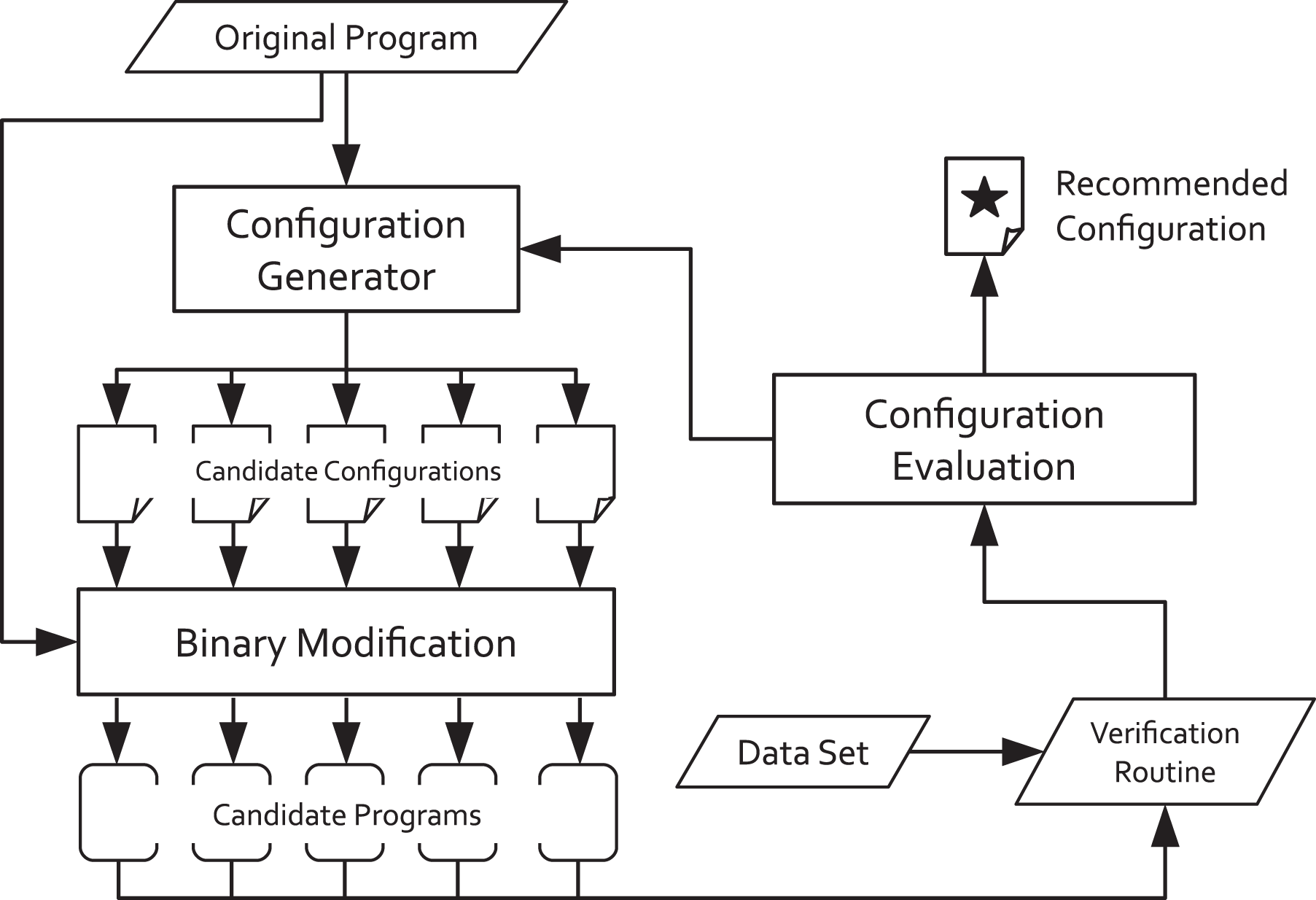
Automatic search overview.

For this analysis, the tuning parameter domain of precision levels consists of the integer values between 0 and 52 (double precision). This domain results in a large search space, since there are 52ⁿ total possible configurations to test with n floating-point instructions, rather than 2ⁿ as reported in previous work. There are also the n log n configurations of aggregate structures such as basic blocks, functions, and modules. However, the breadth-first nature of the search means that the search will obtain overall precision results for the larger program structures first. For instance, the search will first determine the lowest precision level required by the entire program, followed by the lowest precision level required by individual modules, and so on. Thus, the search functions as a refining process, with the results becoming more detailed as more tests are executed. In this way, the search need not run to completion to be useful.

We also use several techniques to reduce the search space and improve search convergence speed. These techniques include the following.

Using a binary search for the precision level of each program component, rather than testing every possible precision level. This alternate approach works because the precision levels are ordered and because we can assume that if x>y, then an instruction executed with x bits of precision will be more accurate than the same instruction executed with y bits of precision. The binary search will find the smallest precision level that passes verification for that component in at most six (⌈log₂ 52⌉) steps. This approach significantly reduces the search space.

Discontinuing the breadth-first search when the precision level of the search point in question falls below a given threshold. The default threshold is 23 bits, which represents single-precision arithmetic. This value is the default because we assume that the most common use case is replacing double-precision arithmetic with single-precision arithmetic rather than half-precision arithmetic or any other level lower than single precision. Thus, the user is unlikely to need the exact precision level requirement once they know that the level is less than 23 bits. This behavior can be disabled if the user desires full sub-single-precision-level information.

Discontinuing the breadth-first search when the runtime instruction execution percentage of the search point in question falls below a given threshold. This metric measures each program point for its contribution to the total number of floating-point instructions executed during the program’s runtime. Applying a threshold to this metric causes the search to focus on the parts of the program that dominate its runtime execution. By default, this option is not enabled, since the appropriate value will vary depending on the target application. In practice, we find that setting this threshold at around 5–10% reduces the overall search time significantly while having an insignificant impact on the results (see Section 3.3).

Providing an option for skipping the top-level (whole-program) configurations, because the overhead will be high relative to subsequent runs due to the high number of extra truncations. The information gained by their analysis is also of minimal interest, because the end goal is to determine precision sensitivity for the subcomponents of a program.

Allowing the search to use cached results from previous searches to expedite the current search. Used in conjunction with the runtime execution threshold and the top-level configuration skip described in previous paragraphs, the user may run a search with little initial time commitment. For instance, the user could skip the application level, and stop the search before it explores any program point responsible for less than an arbitrary share (say 5%) of the program’s execution. In our experience, such a search could take as little as an hour. After the initial search, the user may choose to look deeper by decreasing the runtime execution threshold. The new search can be configured to use the results from the initial search, essentially bypassing all of the tests run by the first search and avoiding any work duplication. We use the term “incremental search” to refer to a search that runs in several iterations using different percentage thresholds, with each iteration utilizing the result caches from previous iterations to avoid test duplication.

2.2 Reduced-precision configurations

Reduced-precision arithmetic can be approximately simulated by reducing the significand to the desired number of bits after each operation. This simple insight provides a way to simulate precisions with levels up to the original precision with minimal program modification. We chose to use truncation rather than rounding because it is faster, simpler to implement, and more conservative than rounding. Rounding would require multiple floating-point instructions (each of which could take multiple clock cycles), while truncation can be done with a single bit-wise integer mask instruction (which often can be done in a single clock cycle). The exponent is unaffected in the current implementation.

We provide a basic configuration file format to allow the user to specify the number of bits for each operation. The configuration files are generated by a static analysis pass, and can be modified manually or via an automatic search routine discussed in subsequent sections. Figure 3 shows an example excerpt from a reduced-precision configuration file. The lines beginning with a caret represent machine code instructions in the program binary, while the other lines give specific precision levels (in bits) for the instructions that will be modified. A unique instruction ID provides a link between these two kinds of lines and allows them to appear out of order in the configuration file if it is convenient to do so.

Figure 3.

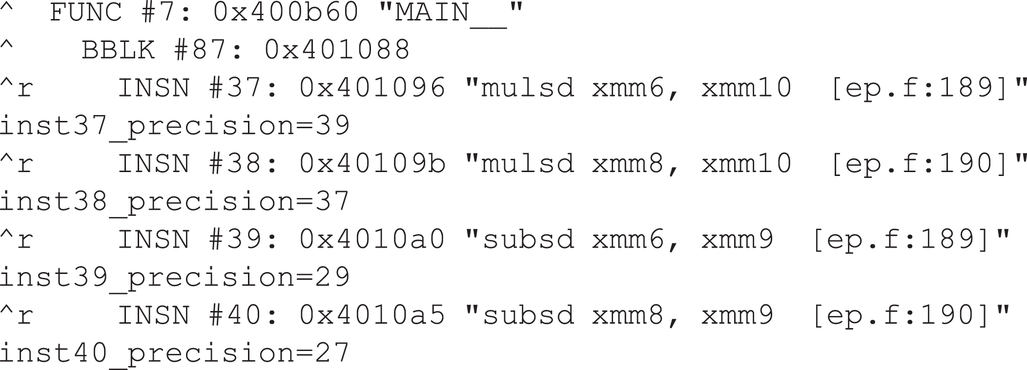
Example of reduced-precision configuration.

The bit values range between 0 and 52. Zero indicates that all of the stored significand should be wiped, leaving the single implied bit to represent a numerical value of one raised to the existing exponent. A bit value of 52 indicates that the entire significand should be preserved, and no truncation is done. The other bit value of particular interest is 23, which represents the number of bits allowed by single precision, and represents a rough estimate of single-precision arithmetic. In fact, it would be a conservative estimate because true single-precision arithmetic would be rounded instead of truncated. The exponent is left unchanged, for both speed and simplicity.

2.3 Binary modification

To reduce the precision of an individual instruction, we augment it by adding code after the instruction that uses bit masking to truncate the resulting floating-point value to the desired number of bits. For instance, if the desired number of bits is 40, then the floating-point value is masked using the binary value 0xfffffff ffffff000, which leaves all bits intact except for the last 12 (52 − 40 = 12).

Figure 4 contains an example of a reduced-precision truncation snippet to give a general sense of what kinds of operations these snippets contain. In this case, the configuration has specified that this instruction (an addition of two XMM registers) should be truncated to 23 bits (roughly single precision). The original instruction comes first, unmodified, followed by the truncation snippet. The snippet is surrounded by save and restore instructions to avoid clobbering registers or unintentionally modifying program state (in Figure 4, these guard instructions preserve the value of %rax and %xmm15). The snippet then loads a temporary XMM register with the appropriate mask constants and does the actual truncation using a bitwise AND instruction.

Figure 4.

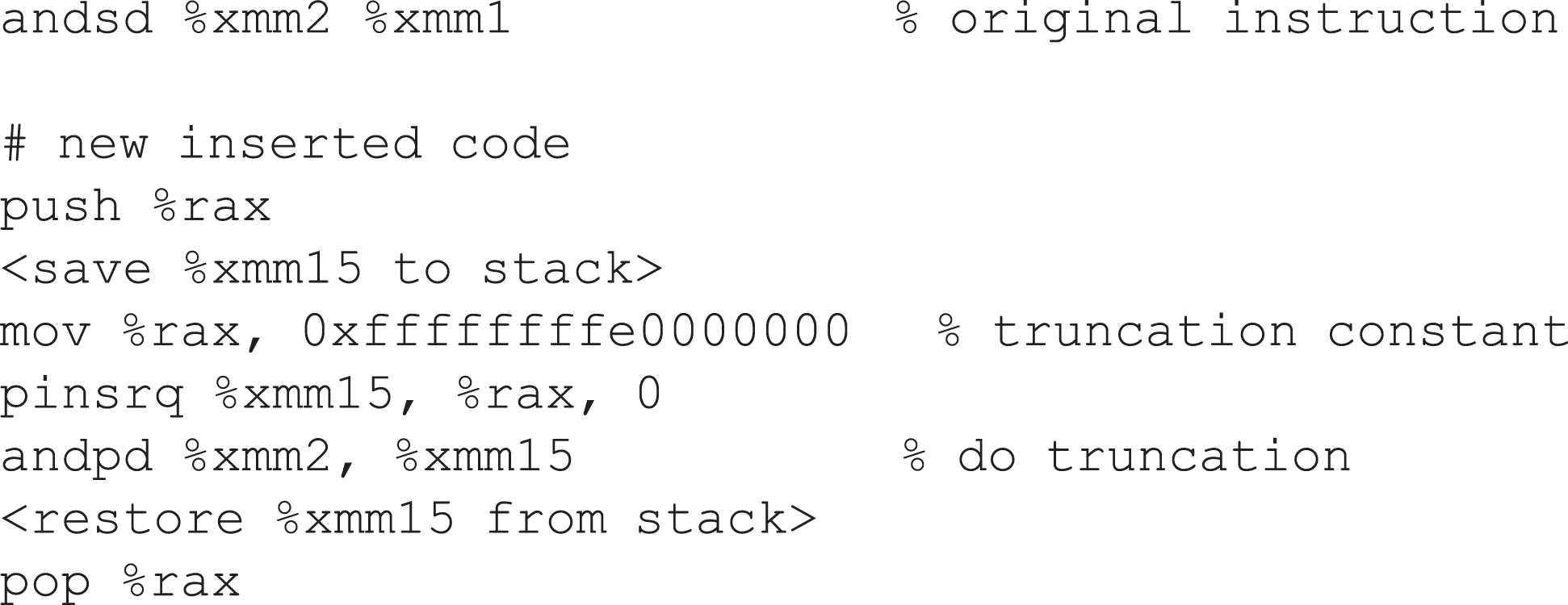
Example reduced-precision replacement snippet.

These snippets impose far less overhead than the snippets required by the mixed-precision analysis described in previous work (Lam et al., 2013). In part, this reduced overhead is because the snippets are simpler, requiring a smaller amount of state to be saved. Also, the reduced-precision snippets do not need to do any kind of floating-point conversion, while the mixed-precision snippets do. In a later section, we show that running a search with this type of analysis is significantly faster than running the corresponding search with mixed-precision analysis.

2.4 Visualization

Our previous work (Lam et al., 2013) reports mixed-precision replacement rates representing the percentage of floating-point instructions (or instruction executions) that could be replaced individually with single-precision and still pass verification. The replacement percentage provided a rough estimate of how much of a program can be replaced with lower precision. However, this percentage is a coarse-grained statistic. To gain any further insight, the developer must look into individual, detailed program component results. This lack of a middle ground illustrates a need for a presentation of precision analysis results at a finer grain than whole-program replacement percentage, while still in a more succinct form than the details for an entire program hierarchy.

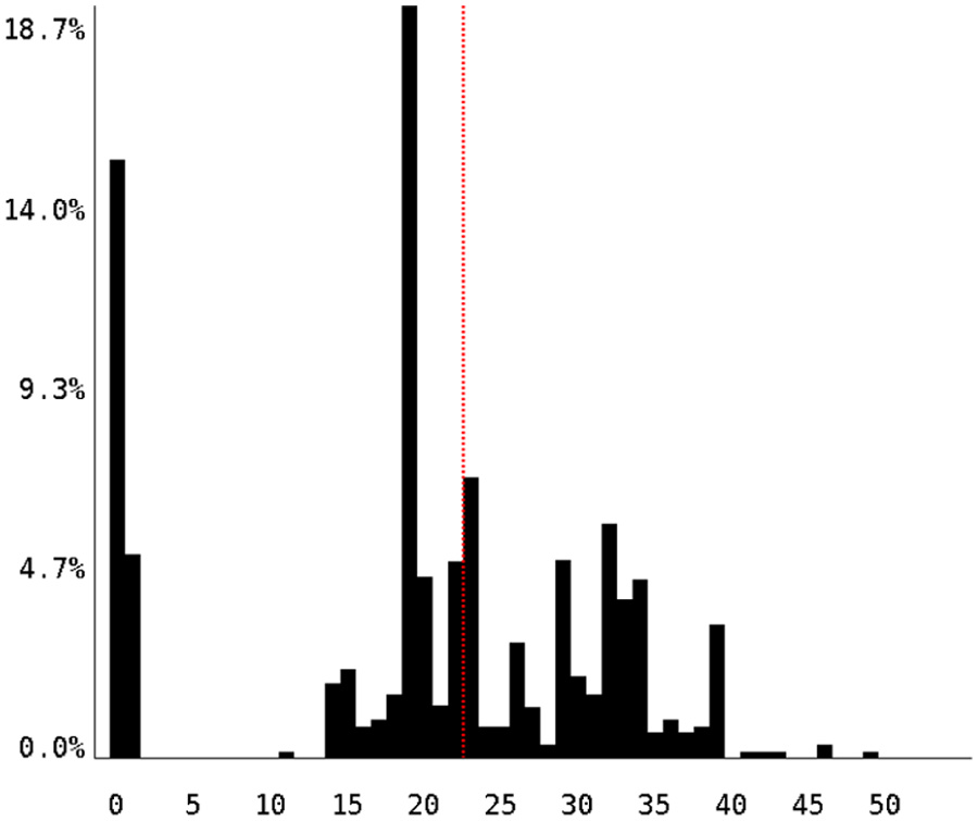
To address this need, we provide a novel histogram-based visualization of whole-program sensitivity. The histograms provide an overview of a program’s floating-point sensitivity profile, providing a better picture than a single percentage while not overwhelming the viewer with details. Figure 5 shows an example histogram from the MG NAS benchmark.

Figure 5.

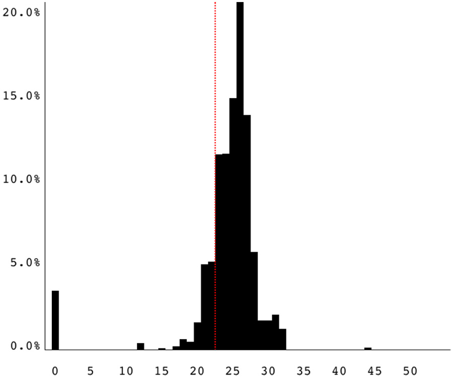
Reduced-precision histogram.

The histogram shows the percentage of floating-point instructions executed (vertical axis), grouped into bars by their final reduced-precision configuration value (horizontal axis). The exact values on the vertical axis are less important than the relative sizes of the bars and their location on the horizontal axis. This visualization provides an easily digestible, at-a-glance overview of a program’s precision level sensitivity.

If the distribution lies mainly to the left of the red bar, then the program is rarely dependent on full double precision. A clustering around the extreme left side of the graph indicates that most of the program uses relatively little precision, showing a high potential for single-precision replacement. Conversely, a clustering around the extreme right side of the graph indicates that most of the program relies on full double precision, indicating little chance for a mixed-precision implementation without major rewriting. A clustering around the red bar is perhaps the most interesting outcome, since it implies that the program needs just barely more than single precision accuracy, implying that perhaps a small amount of algorithmic reconfiguration could enable the use of single-precision arithmetic for large portions of the computation.

The histogram values can optionally be binned into a smaller number of bars, and the zero-precision bar (i.e. floating-point computation that has been determined to be non-essential for the final computation) can be excluded. In the results we present in this paper, we leave the values in their original bins (i.e. a bar for each precision level) to preserve all trends in the original data, and we include the zero-precision bar for completeness. The histogram also includes a red, dotted bar at 23 bits, which represents the cutoff for single precision.

Our visualization interface can also build histograms by precision level of the number of binary floating-point instructions, as opposed to the runtime execution count. This difference corresponds to the distinction between static and dynamic percentages in mixed-precision analysis. However, we have focused on the dynamic instruction execution count because of its greater relevance to overall performance.

The results of an automated reduced-precision search are also visualized in a GUI using colors as shown in Figure 6. This interface allows the user to browse a program’s control structure to identify the lower-precision areas by their graphical appearance (more green than red) and to drill down quickly into the regions of interest. These include regions with consistently high-precision requirements that may benefit from higher precision or algorithmic changes, as well as regions with low-precision requirements that can probably be replaced with lower precision arithmetic. This interface allows the user to drill down and look at individual component results that are of interest after viewing the overall histogram representation.

Figure 6.

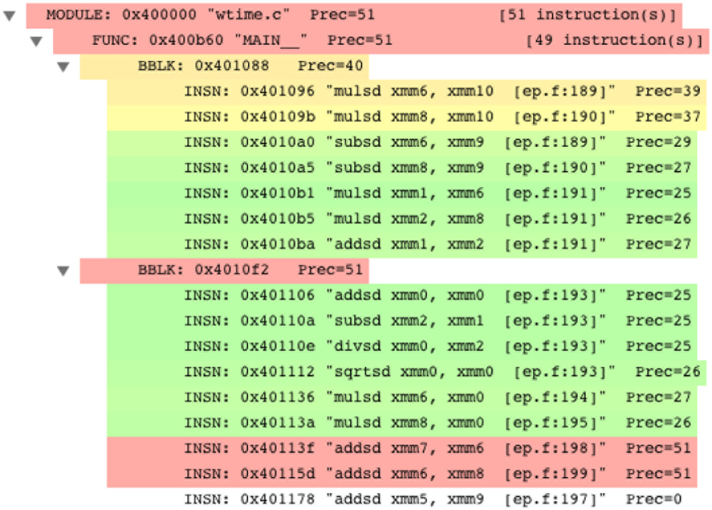
Reduced-precision configuration viewer.

3 Results

In this section, we present results using our analysis techniques. First, we show via experimentation the runtime overhead on several standard benchmarks for real workloads, and that our technique improves on previous results. Second, we show through various case studies how our technique can inform developers about the floating-point behavior of their program and its sensitivity to roundoff error.

3.1 Overhead benchmarks

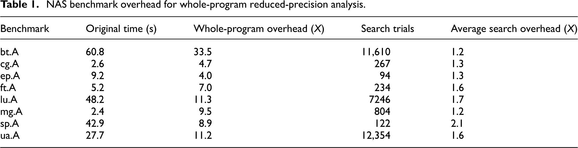
Table 1 shows instrumentation overhead results from the NAS benchmark suite (Bailey et al., 1995, 1991: see also http://www.nas.nasa.gov/publications/npb.html). For these single-core trials, the benchmarks were compiled using the Intel compiler version 12.1.4 with -O3 optimization. The table gives two overhead numbers. The first overhead number (third column) is from running whole-program reduced precision analysis, averaged over five runs each. The analysis was configured to use 52-bit precision so that the overhead could be measured without affecting the program’s execution. The second overhead number (fifth column) is from running an automatic search on the entire program. The fourth column reports the total number of trials, and the fifth column is the overhead averaged over all of those trials. Since many trials apply reduced-precision analysis to only a few instructions, the overhead is much lower.

Table 1.

NAS benchmark overhead for whole-program reduced-precision analysis.

Benchmark	Original time (s)	Whole-program overhead (X)	Search trials	Average search overhead (X)
bt.A	60.8	33.5	11,610	1.2
cg.A	2.6	4.7	267	1.3
ep.A	9.2	4.0	94	1.3
ft.A	5.2	7.0	234	1.6
lu.A	48.2	11.3	7246	1.7
mg.A	2.4	9.5	804	1.2
sp.A	42.9	8.9	122	2.1
ua.A	27.7	11.2	12,354	1.6

3.2 Mixed-precision comparison

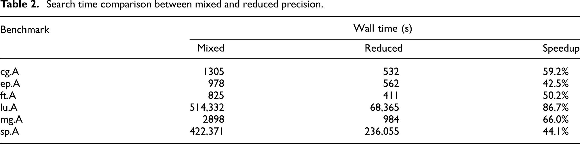
To compare the overhead for reduced-precision analysis with the overhead for mixed-precision analysis, we replicated previous work (Lam et al., 2013) by adding the capability to run mixed-precision searches using reduced-precision instrumentation. To implement this capability, we added a new mode for mixed-precision search that does 23-bit reduced-precision replacement wherever the search would normally call for single-precision replacement. Where the search would normally call for double-precision replacement, we instead do 52-bit reduced-precision replacement, which normally becomes optimized to a no-op since no bits are truncated. This mode significantly reduces the number of instructions that are generated to replace the old instructions, partially because double-precision replacement usually becomes a no-op and partially because the 23-bit reduced-precision snippets are much simpler than the regular mixed-precision replacement snippets.

Table 2 shows the speedup using this mode as measured by the overall search wall time, which ranged from several minutes to several days depending on the benchmark. All searches were run using multiple search threads, and the number of threads was kept constant between the original mixed-precision and reduced-precision runs. The speedup consistently ranged between 40% and 70%, a significant improvement.

Table 2.

Search time comparison between mixed and reduced precision.

	Wall time (s)
Benchmark	Mixed	Reduced	Speedup
cg.A	1305	532	59.2%
ep.A	978	562	42.5%
ft.A	825	411	50.2%
lu.A	514,332	68,365	86.7%
mg.A	2898	984	66.0%
sp.A	422,371	236,055	44.1%

We also examined how closely the results matched the original mixed-precision searches. Since 23-bit replacement is only a rough approximation of single precision, we did not expect the results to be identical. However, in most of the benchmarks the results were similar, with less than a 10% difference in the number of instruction executions requiring double precision.

For two benchmarks (MG and SP), we found a roughly 20% difference in the results. In these results, the floating-point instruction executions that required higher precision are explained by the conservative nature of reduced precision due to truncation, while the executions that required lower precision are attributed to the corresponding noise caused by different search paths through the parameter space. This experiment shows that reduced-precision analysis can dramatically reduce the time required to run mixed-precision searches, while still achieving similar results.

This experiment also suggests that a hybrid approach might yield even better results. One could run the reduced-precision search first to get a general estimate of sensitivity, and then run full mixed-precision searches on select subsets of the program to get more accurate results. This approach would be a more complex variant of the incremental search described in the previous section. Our framework provides the capability for such a hybrid approach, but more research would be required to determine the best point to transition between strategies.

3.3 NAS benchmarks

Figure 7 shows histogram results for selected NAS benchmarks (Bailey et al., 1995, 1991: see also http://www.nas.nasa.gov/publications/npb.html). These graphs give a more complete picture of the benchmarks’ relative precision sensitivities than do the single percentages from previous work (Lam et al., 2013). Some benchmarks (such as BT and LU) show a strong potential for mixed-precision configurations, with large portions of their sensitivities under the single-precision level. These results match the high replacement percentages from previous work (Lam et al., 2003), Conversely, some benchmarks (such as CG and FT) clearly require more than single precision for most of their computation; thus, these benchmarks seem to have little opportunity for a comprehensive mixed-precision implementation without a major algorithmic shift. Again, these results match the low replacement percentages from previous work (Lam et al., 2013). Other benchmarks (such as MG and UA) have a clustering of sensitivities around the single-precision mark, indicating that if the computation could be rewritten to be slightly less sensitive, the benchmark has a large potential for using single precision.

Figure 7.

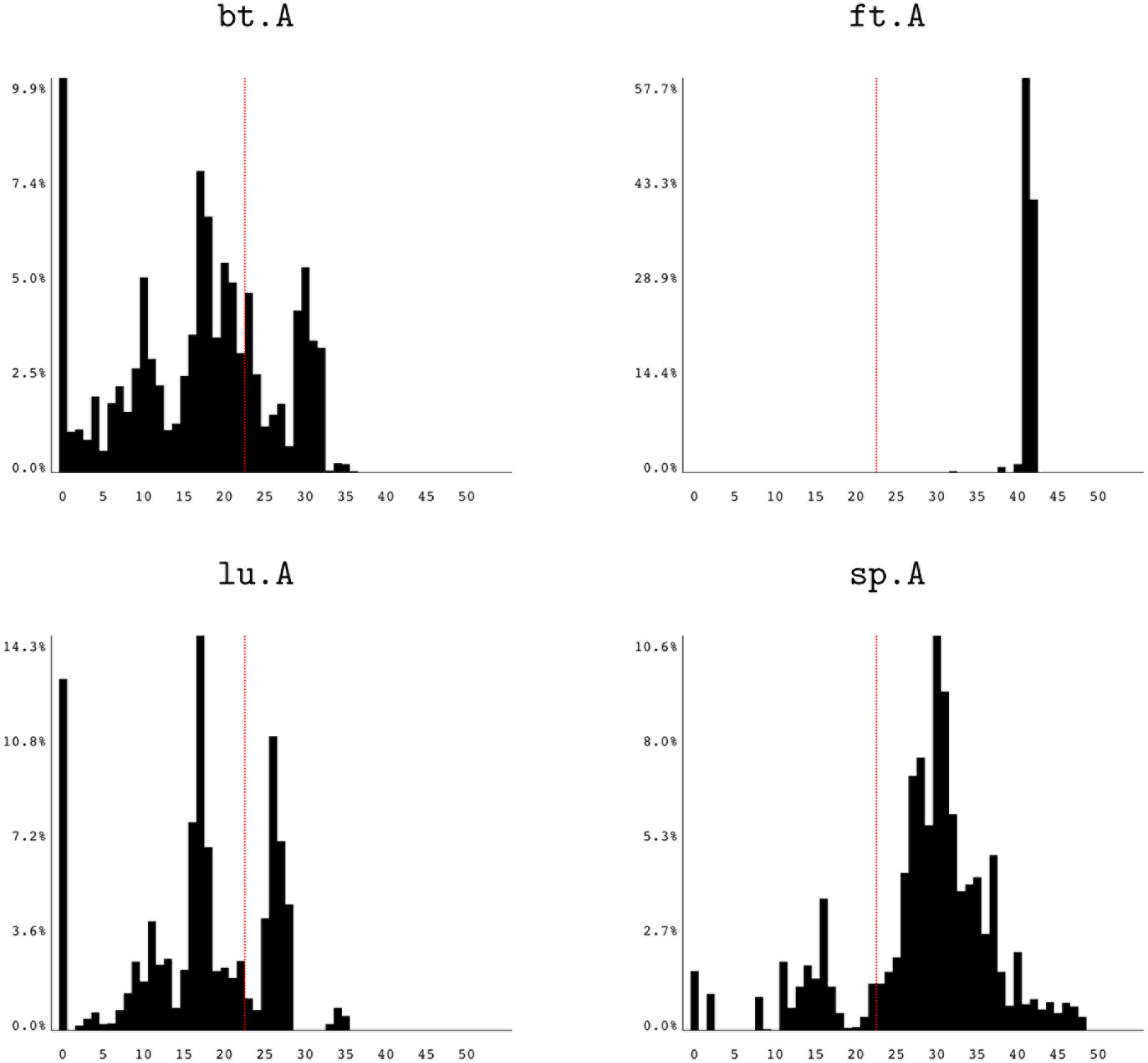
Reduced-precision histograms for NAS benchmarks.

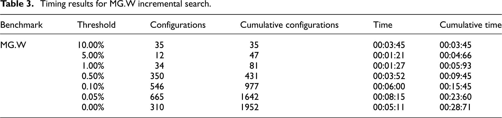
Figure 8 shows several histograms from running an incremental search on MG.W from the NAS benchmarks. Table 3 provides the corresponding search wall times and configuration counts, including the number of configurations tested at a particular increment as well as the cumulative number of configurations tested over the entire search. The histograms show a pattern of refinement that we found to be typical of incremental search results, with the curve beginning heavily-weighted towards the right side of the graph and gradually migrating towards the left as more and more of the program is explored in detail. By the time the search explores any program point accounting for 0.5% or more of the program’s instruction executions, the graph closely resembles its final form. Thus, the user may stop the search once the incremental results are no longer adding information.

Figure 8.

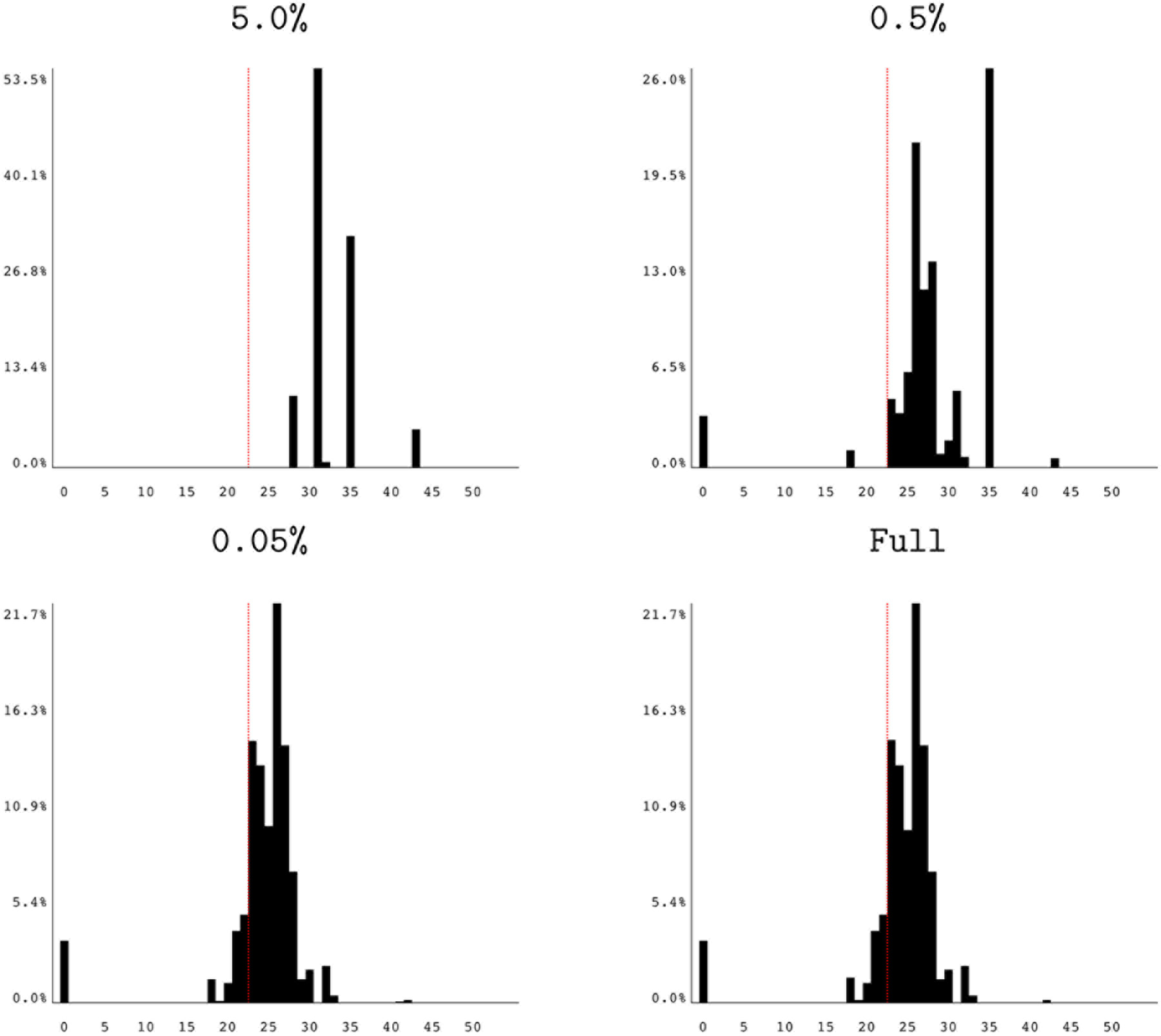
Reduced-precision histograms for MG.W incremental search.

Table 3.

Timing results for MG.W incremental search.

Benchmark	Threshold	Configurations	Cumulative configurations	Time	Cumulative time
MG.W	10.00%	35	35	00:03:45	00:03:45
	5.00%	12	47	00:01:21	00:04:66
	1.00%	34	81	00:01:27	00:05:93
	0.50%	350	431	00:03:52	00:09:45
	0.10%	546	977	00:06:00	00:15:45
	0.05%	665	1642	00:08:15	00:23:60
	0.00%	310	1952	00:05:11	00:28:71

3.4 LAMMPS results

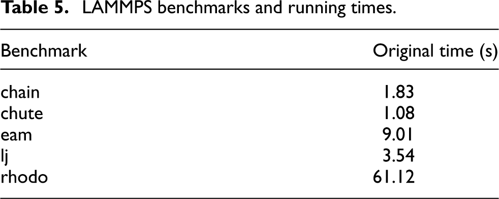
We ran tests on LAMMPS, a molecular dynamics code that is part of the ASC Sequoia benchmark suite (ASC Sequoia Benchmark Codes, available at https://asc.llnl.gov/sequoia/benchmarks/). In these tests, we show that we can obtain precision information about a program in a reasonable amount of analysis time. We examined the “30Aug13” version of LAMMPS with four provided benchmark work loads: chute, eam, lj, and rhodo. We built the LAMMPS binary with the default compiler (GCC) and the default optimization levels; it contained 56,643 candidate instructions for reduced-precision replacement. Table 5 shows the original runtimes of the benchmarks.

For each benchmark, we ran several incremental reduced-precision searches, initializing the runtime percentage threshold at 10% and gradually lowering it to 5%, 1%, and finally 0.5%. Each individual search used the results of the previous searches as a cache, allowing it to skip directly to the incremental tests for the new threshold. We also skipped the application-level tests for these benchmarks, since they incur a large overhead and only yield information that can be deduced from lower-level results.

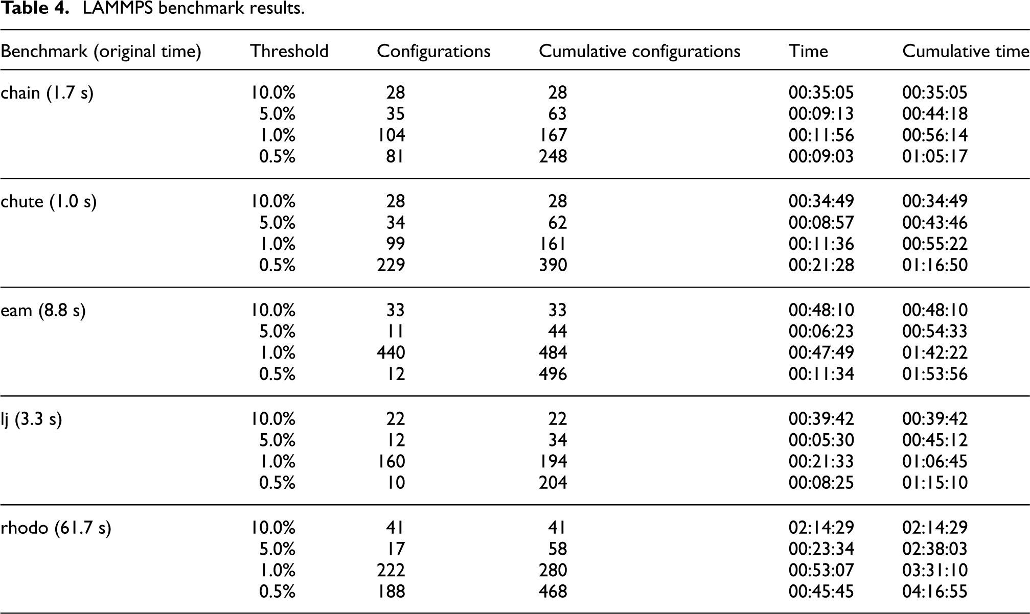
Table 4 shows the timing results of these tests, and Figure 9 shows the final histograms for each benchmark. For the timing results, we see the same general pattern as in Table 3. The number of configurations tested (and therefore the time spent) at every iteration of the search varies, but does not increase dramatically in later iterations. This pattern suggests a “leveling off” of the search, indicating that further computation would be unhelpful. The time spent in individual iterations matches this trend.

Table 4.

LAMMPS benchmark results.

Benchmark (original time)	Threshold	Configurations	Cumulative configurations	Time	Cumulative time
chain (1.7 s)	10.0%	28	28	00:35:05	00:35:05
	5.0%	35	63	00:09:13	00:44:18
	1.0%	104	167	00:11:56	00:56:14
	0.5%	81	248	00:09:03	01:05:17

chute (1.0 s)	10.0%	28	28	00:34:49	00:34:49
	5.0%	34	62	00:08:57	00:43:46
	1.0%	99	161	00:11:36	00:55:22
	0.5%	229	390	00:21:28	01:16:50

eam (8.8 s)	10.0%	33	33	00:48:10	00:48:10
	5.0%	11	44	00:06:23	00:54:33
	1.0%	440	484	00:47:49	01:42:22
	0.5%	12	496	00:11:34	01:53:56

lj (3.3 s)	10.0%	22	22	00:39:42	00:39:42
	5.0%	12	34	00:05:30	00:45:12
	1.0%	160	194	00:21:33	01:06:45
	0.5%	10	204	00:08:25	01:15:10

rhodo (61.7 s)	10.0%	41	41	02:14:29	02:14:29
	5.0%	17	58	00:23:34	02:38:03
	1.0%	222	280	00:53:07	03:31:10
	0.5%	188	468	00:45:45	04:16:55

Figure 9.

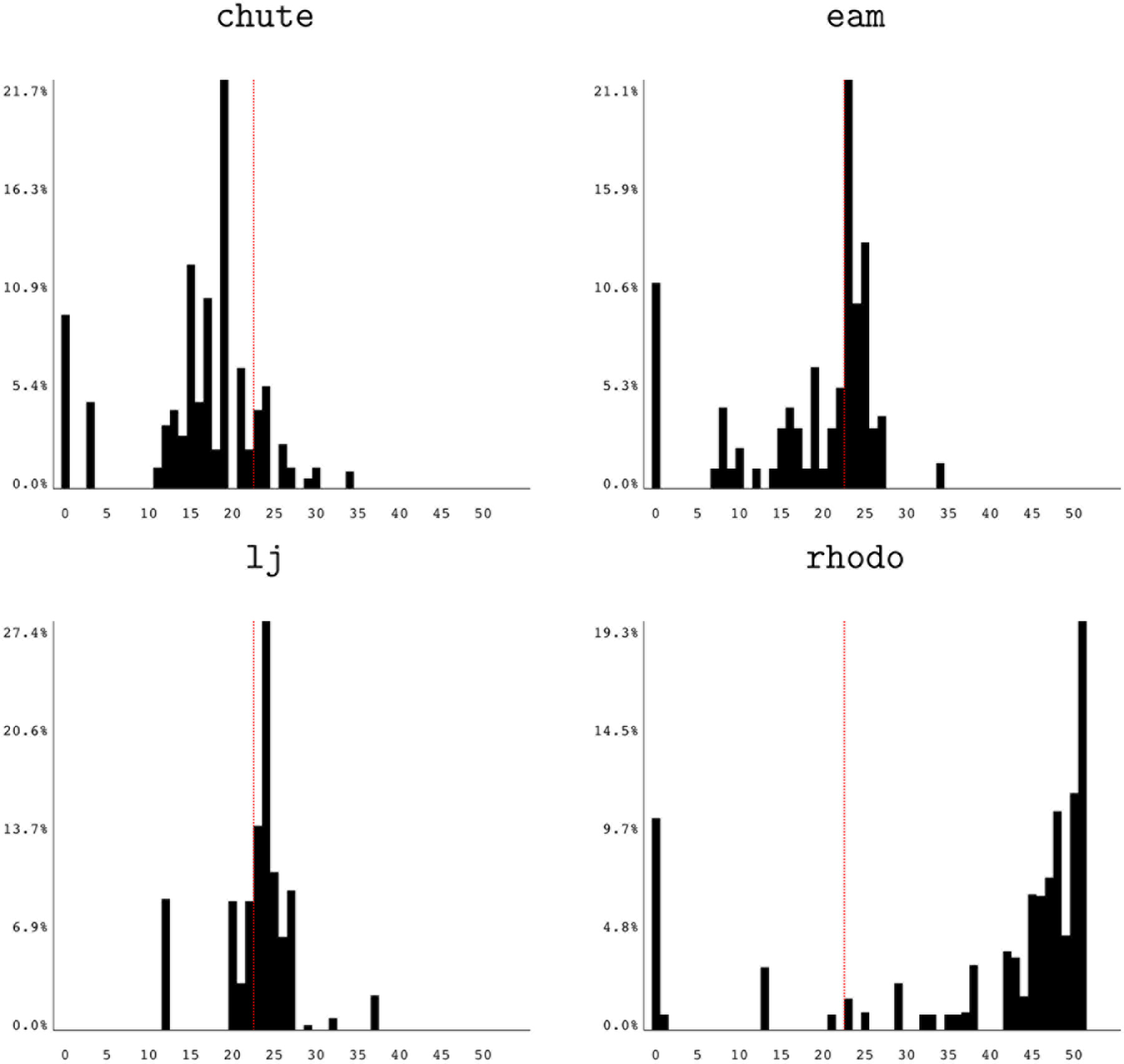
Reduced-precision histograms for LAMMPS benchmarks.

The total number of configurations tested does vary, but there are no severe outliers; even benchmarks with widely differing profiles (such as “eam” and “rhodo”) test similar numbers of configurations. The total wall time varies as expected with both the number of configurations tested and the original running time of the benchmark itself. The final histograms show a range of precision sensitivity, reinforcing again that floating-point behavior is highly sensitive to particular data sets.

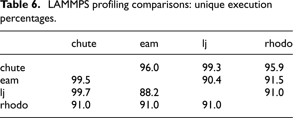
To further explore this variance due to program input, we compared execution profiling data between runs. Table 6 shows the percentage of floating-point instruction executions that were unique to the row-specific benchmark when compared with the column-specific benchmark. Uniqueness is determined using the instruction addresses in the binary. For instance, 96.0% of the floating-point instruction executions in the “chute” benchmark are attributed to instructions that were never executed in the “eam” benchmark. The high percentages throughout the table show that the benchmarks exercise highly disjoint portions of the full application, partially explaining the widely varying precision sensitivity results. The disjoint execution profiles are largely due to the benchmarks using different force update functions for molecular movement. In the future, it would be interesting to explore further analysis of program variance due to differing inputs. For now, the runtime nature of our analysis ensures that such behaviors are captured, provided that the analysis incorporates data sets that are representative of target use cases.

The LAMMPS experiment also shows the utility of our visualization. We quickly noticed that the histograms for two data sets varied considerably, leading us to further investigate profiling data on the hypothesis that the benchmarks might be exercising different program paths. This process shows how a developer might be able to gain insight from visualization and apply it to pursue deeper analysis.

We also looked at the overall runtime of our search process. Usually, we were able to get results in under an hour for all portions of the program representing over 5% of the total floating point instructions executed. This timing result shows that the analysis crosses an important threshold for practical viability. Even for the benchmark that took over a minute to run initially, we had results at the 5% level in under three hours. These experiments show that our reduced-precision analysis techniques provide the user with the capability to choose the granularity of the search and to benefit from a corresponding reduction in the time to solution.

3.5 HPCCG results

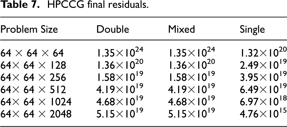
In this section, we present a result obtained by analyzing HPCCG, a conjugate gradient code. The original program uses double-precision arithmetic. For the purposes of experimentation, we created a version that used only single precision for computation. The single-precision version was slightly faster but three significant digits less precise in its final residual.

We ran several reduced-precision searches on the original program using multiple data sizes. One consistent result emerged from all searches: one particular function (ddot) was the crucial point for precision preservation. We manually examined that function and found that it performed a summation across the entire grid. We created a very simple mixed-precision version of this code by changing that function to use double precision for the summation, while all the rest of the program used single precision. We then tested the resulting configuration by running it on various problem sizes in the same manner as the tests provided by the benchmark authors. All experiments were done on a single node for simplicity.

As can be seen in Table 5, the resulting mixed-precision version had a final residual that was much closer to that of the original double-precision program than the single-precision version. In fact, the residuals were identical to the number of digits printed by the program, implying that the result would be acceptable to the original author. This variant was created without any domain-specific knowledge and was informed solely by the results from the reduced-precision search. Although the resulting mixed-precision variant was not immediately faster, it did demonstrate a level of precision that was very close to the original program despite doing much of its computation in single precision. We anticipate that a domain expert could use these results to further improve the performance of the program.

Table 5.

LAMMPS benchmarks and running times.

Benchmark	Original time (s)
chain	1.83
chute	1.08
eam	9.01
lj	3.54
rhodo	61.12

Table 6.

LAMMPS profiling comparisons: unique execution percentages.

	chute	eam	lj	rhodo
chute		96.0	99.3	95.9
eam	99.5		90.4	91.5
lj	99.7	88.2		91.0
rhodo	91.0	91.0	91.0

Table 7.

HPCCG final residuals.

Problem Size	Double	Mixed	Single
64 × 64 × 64	1.35×10²⁴	1.35×10²⁴	1.32×10²⁰
64× 64 × 128	1.36×10²⁰	1.36×10²⁰	2.49×10¹⁹
64× 64 × 256	1.58×10¹⁹	1.58×10¹⁹	3.95×10¹⁹
64× 64 × 512	4.19×10¹⁹	4.19×10¹⁹	6.49×10¹⁹
64× 64 × 1024	4.68×10¹⁹	4.68×10¹⁹	6.97×10¹⁸
64× 64 × 2048	5.15×10¹⁹	5.15×10¹⁹	4.76×10¹⁵

3.6 CLAMR results

Finally, we present results based on analysis of a scientific computing code called CLAMR, which is a proxy application for cell-based adaptive mesh refinement (see https://github.com/losalamos/CLAMR). The specific application we examined was a cylindrical dam break problem with two-dimensional shallow water equations. This code introduced a novel approach to load balancing using a stencil-based refinement method, as well as a new Cartesian-indexed hash mapping scheme for efficient neighbor access (Nicholaeff et al., 2013).

CLAMR has several different versions for single-core CPUs, distributed systems (OpenMP, MPI, and hybrid), and accelerators (OpenCL for GPUs and hybrid MPI/OpenMP for Intel MIC). In this experiment we looked primarily at the single-core and GPU versions, and we worked closely with the code author. For the actual searches, we used the single-core CPU version because some of our library dependencies do not have any GPU implementation, but we performed testing runs using the GPU version. Before running a search, we manually converted a few global state structures to be stored in single precision. Then, we created a verification routine that checked the final mass sum to seven decimal digits and the time step to the full reported precision, which the code author determined to be sufficient accuracy.

We ran a full reduced-precision search, and the resulting histogram can be seen in Figure 10. There are a large number of executions that fall just under the single-precision cutoff, which was a promising result. In addition, the declining tail of instructions that require higher precision looked rather innocuous, lacking the right-side clumping that we have seen in results for other applications (for instance, the “rhodo” workload for LAMMPS). The results also included some concrete suggestions regarding which functions might be good candidates for single-precision conversion.

Figure 10.

CLAMR histogram.

CLAMR, as a proxy application, is a relatively bare-bones simulation code and most of its computation is critical to the simulation fidelity. Thus, we found relatively few places to reduce precision in computation. However, we achieved a significant reduction in storage costs by converting several important large matrices to single precision. For the default problem size, the reduction is around 25%; for additional physics, such as more materials, the memory savings would approach 50% (a factor of two). Reducing the storage size yields concrete benefits in reduced cache pressure and faster I/O for graphics output and checkpoint/restart files.

In the end, the code author built three versions of the code at three different precision levels: full, mixed, and minimum. Our analysis helped to inform the decisions on how to create the three levels in a consistent manner. Without the analysis, it would have been guesswork as to where precision needed to be maintained.

In the future, these three versions can be used to improve the efficiency of simulations on high-performance machines. Exploratory runs can be done at minimum precision with scoping runs for large ranges of parameter sweeps, followed by mixed precision runs to focus in on the areas of interest (while still saving storage costs), and then full precision for the final simulation run. Both CPU time and storage overhead can be reduced with this approach.

4 Related work

4.1 Backwards and forwards error analysis

The analysis efforts regarding floating-point representation and its accompanying roundoff error initially focused on manual backward and forward error analysis. An early work in this area was published in 1959 (Carr, 1959) and Wilkinson’s seminal work was published in 1964 (Wilkinson, 1964). More recent summaries include Goldberg (1991) and Overton (2001) on IEEE arithmetic, and Higham (2002: chapters 1, 2, 26, and 27) on error analysis.

Forward error analysis begins at the input and examines how errors are magnified by each operation. Backward error analysis is a complementary approach that starts with the computed answer and determines the exact floating-point input that would produce it. Backward analysis is done because it is usually difficult to obtain good forward error bounds. Both techniques provide an indication of how sensitive the computation is, and how incorrect the computed answer might be. Computations that are highly sensitive are called ill-conditioned.

The book by Higham (2002) gives backward and forward error analyses for a number of algorithms and conditioning theory for a number of numerical analysis problems. Without an error analysis background, however, these analyses are not easily applicable to many situations a numerical programmer might encounter.

4.2 Interval and affine arithmetic

Researchers have attempted to model the behavior of a floating-point program using a technique called “interval arithmetic” (Krämer, 1998), which represents every number x in a program using a range $\bar{x} = [x . lo, x . hi]$ instead of a fixed value. Unfortunately, regular interval arithmetic is not always useful due to the quick compounding of errors (Andrade et al., 1994), and the difficulty of handling intervals containing zero (Higham, 2002). In the worst case, division by zero will produce an invalid interval, or the interval will eventually expand to $(- \infty, + \infty)$ , a result that is trivially correct but practically useless. Even in less-extreme circumstances, however, the average-case error is rarely as bad as the worst case, and so interval analysis by itself is usually of little value to programmers who are merely interested in the practical behavior. Interval arithmetic was later improved by Andrade et al. (1994) and others with the concept of “affine arithmetic,” replacing the ranges of interval arithmetic with a linear combination of error factors. Affine representation preserves information about error independence, and allows some errors to cancel out others. Thus, the bounds for the result are tighter than those that would be obtained in standard interval arithmetic, but they are still more pessimistic than the results obtained by our technique because they attempt to capture all possible executions rather than representative executions.

More recently, Goubault et al. (2002), Martel (2007), and others have built abstract semantics and static analyses using affine arithmetic. In addition, work by Martel (2009) describes a system that can do program transformations to increase accuracy. Unfortunately, these static analyses are still not dataset-sensitive, and still give conservative estimates that may not be useful. In addition, they require some manual tuning by the programmer, particularly with regards to the extent that loops are unrolled: more unrolling produces better answers but requires more lengthy analyses. These techniques also only work for a subset of language features (often excluding high-performance computing (HPC)-specific interests such as MPI communication), and are usually limited to C programs. Finally, these techniques merely make observations about error, and do not aid the programmer in building mixed-precision variants of their code.

4.3 Manual mixed precision

More recently, many researchers (Anzt et al., 2010; Buttari et al., 2007; Clark et al., 2010; Göddeke et al., 2007; Li et al., 2002) have demonstrated that mixed precision can achieve the same results as using purely double-precision arithmetic, while being much faster and memory efficient. They usually present linear solvers (particularly sparse solvers) as examples, showing how most operations can be run in single precision. These solvers have been applied to a wide range of problems, including fluid dynamics (Anzt et al., 2010), lattice quantum chromodynamics (Clark et al., 2010), and finite element methods (Göddeke et al., 2007). Often, GPUs are cited as the target of these optimizations because of their streaming capabilities (Anzt et al., 2010; Clark et al., 2010).

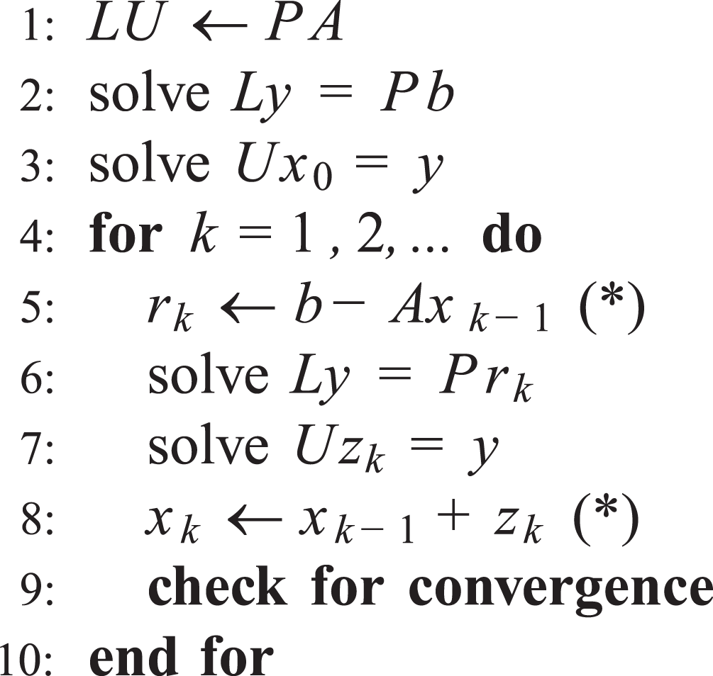
In the iterative algorithm shown in Figure 11, for example, only the steps marked with asterisks (lines 5 and 8) must be executed in double precision. The authors note that all $O (n^{3})$ steps can be run in single precision, while the double-precision steps are only $O (n^{2})$ . Thus, using mixed precision can yield significant performance and memory bandwidth savings. On the streaming Cell processor, for instance, the mixed-precision version performed up to eleven times faster than the original double-precision version. Even on non-streaming processors, they obtained a performance improvement between 50% and 80%.

Figure 11.

Mixed precision algorithm.

Researchers in the field of computer graphics have also found that mixed-precision algorithms can improve performance (Hao and Varshney, 2001). By varying the number of bits used for graphics computations, they report speedups of up to a factor of four or five, with little or no apparent image degradation. They use fixed-point arithmetic, but the mixed-precision concepts are similar to floating-point. Unfortunately, these techniques do not automatically generalize to other domains because they involve specialized vertex and lighting calculations.

In recent work, Jenkins et al. (2012) describe a novel scheme for reorganizing data structures by numerical significance. Their technique splits up a floating-point number into several chunks on byte boundaries. All pieces of corresponding significance are stored consecutively in memory for storage and I/O, and the original numbers are re-assembled only when needed for calculation. Thus, the developer can vary the precision of floating-point data during data movement by truncating the lower-precision blocks. In their experiments, they found that some applications can use as few as 3 bytes (24 bits) of floating-point data and retain an acceptable level of accuracy. This work focused on the I/O implications, however, and did not address the possibility of single-precision arithmetic. Their system also incurs overhead during data re-assembly.

4.4 Automatic mixed precision

In previous work, we developed a framework for automated mixed precision analysis (Lam et al., 2013). In this paper, we have used this framework to implement a more generalized precision level analysis. Subsequent work by Rubio-González et al. (2013) presented similar techniques that work closer to the source level. This work attempts to lower the precision of as many program variables as possible while still passing verification. Their search does not do an exhaustive search of the space, but focuses on finding a smaller number of variables that can be replaced together. Implemented in the LLVM framework, this technique is not immediately applicable to programs built with other compilers.

5 Conclusion

We have described techniques for building reduced-precision configurations of floating-point programs, as well as an automatic search process that identifies the precision-level sensitivity of various parts of an application. We have also described our implementation of these techniques as extensions to the CRAFT framework. These techniques allow developers to be more efficient in analyzing their code by automating the precision replacement tests given user-defined criteria for acceptable precision. Benchmark overhead results indicate that reduced-precision searches are significantly faster than mixed-precision searches. We have also presented a novel histogram-based visualization of a program’s floating-point precision sensitivity. Finally, we showed that an incremental technique provides the user with the ability to choose the granularity of the search and to benefit from a corresponding reduction in the time to solution.

In the future, we plan to extend this analysis, allowing it to refine the final results to produce more comprehensive precision-level recommendations. We also plan to further explore the variances in precision results due to differing program inputs, potentially creating multiple mixed-precision program configurations and dynamically switching between them at runtime. Finally, we plan to pursue the integration of this analysis with other program analysis and modeling techniques.

Footnotes

Acknowledgements

We thank Bob Robey and Nathan Debardeleben from Los Alamos National Laboratory for assistance with the CLAMR case study presented in this paper.

Declaration of Conflicting Interests

The author(s) declared no potential conflicts of interest with respect to the research, authorship, and/or publication of this article.

Funding

The author(s) disclosed receipt of the following financial support for the research, authorship, and/or publication of this article: This work is supported in part by the DOE (grant numbers DOEN.DESC0002351 and DOEN.DES C0002616).

References

Andrade

MVA

Comba

JLD

Stolfi

(1994) Affine arithmetic. In: INTERVAL’94, St. Petersburg, Russia, pp. 1–10.

Anzt

Rocker

Heuveline

(2010) Energy efficiency of mixed precision iterative refinement methods using hybrid hardware platforms. Computer Science Research and Development 25(3–4): 141–148.

Bailey

Harris

Saphir

Wijngaart

RVD

Woo

Yarrow

(1995) The NAS Parallel Benchmarks 2.0. Technical Report 3, The Pennsylvania State University CiteSeer Archives. DOI:10.1177/109434209100500306.

Bailey

Barszcz

Barton

Browning

Carter

Fatoohi

. (1991) The NAS Parallel Benchmarks. International Journal of Supercomputer Applications 5(3): 63–73.

Buck

Hollingsworth

(2000) An API for runtime code patching. Journal of Supercomputing Applications and High Performance Computing 14: 317–329.

Buttari

Dongarra

Kurzak

Langou

Luszczek

. (2006) Exploiting mixed precision floating point hardware in scientific computations. In Selected Papers from the 2006 International Advanced Research Workshop on High Performance Computing and Grids. Cetraro, Italy, pp. 19–36. Available at: http://dblp.uni-trier.de/db/conf/hpc/hpc2006.html

Carr

(1959) Error analysis in floating point arithmetic. Communications of the ACM 2(5): 10–16.

Clark

Babich

Barros

Brower

Rebbi

(2010) Solving lattice QCD systems of equations using mixed precision solvers on GPUs. Computer Physics Communications 181(9): 1517–1528.

Dongarra

Beckman

Moore

Aerts

Aloisio

Andre

. (2011) The International Exascale Software Project Roadmap. International Journal of High Performance Computing Applications 25(1): 3–60.

10.

Göddeke

Strzodka

(2011) Cyclic reduction tridiagonal solvers on GPUs applied to mixed-precision multigrid. IEEE Transactions on Parallel and Distributed Systems 22(1): 22–32.

11.

Göddeke

Strzodka

Turek

(2007) Performance and accuracy of hardware-oriented native-, emulated- and mixed-precision solvers in FEM simulations. International Journal of Parallel, Emergent and Distributed Systems 22(4): 221–256.

12.

Goldberg

(1991) What every computer scientist should know about floating point arithmetic. ACM Computing Surveys 23(1): 5–48.

13.

Goubault

Martel

Putot

(2002) Asserting the precision of floating-point computations: a simple abstract interpreter. In Le Métayer

(ed.) ESOP ’02 Proceedings of the 11th European Symposium on Programming Languages and Systems (Lecture Notes in Computer Science, vol. 2305). Berlin: Springer-Verlag, pp. 209–212.

14.

Hao

Varshney

(2001) Variable-precision rendering. In: Proceedings of the 2001 Symposium on Interactive 3D Graphics (SI3D’01). New York: ACM Press, pp. 149–158.

15.

Ding

(2001) Using accurate arithmetics to improve numerical reproducibility and stability in parallel applications. The Journal of Supercomputing 18(3): 259–277.

16.

Higham

(2002) Accuracy and Stability of Numerical Algorithms (2nd edn). Philadelphia, PA: SIAM.

17.

IEEE (2008) IEEE Standard for Floating-Point Arithmetic (IEEE 754-2008). New York: IEEE.

18.

Jenkins

Schendel

Lakshminarasimhan

Boyuka II

Rogers

Ethier

. (2012) Byte-precision level of detail processing for variable precision analytics. In: Proceedings of the International Conference on High Performance Computing, Networking, Storage and Analysis (SC’12). Los Alamitos, CA: IEEE Computer Society Press.

19.

Krämer

(1998) A priori worst case error bounds for floating-point computations. IEEE Transactions on Computers 47(7): 750–756.

20.

Lam

Hollingsworth

de Supinski

Legendre

(2013) Automatically adapting programs for mixed-precision floating-point computation. In: Proceedings of the 27th International ACM Conference on Supercomputing (ICS ’13). New York: ACM Press, p. 369.

21.

Demmel

Bailey

Henry

Hida

Iskandar

. (2002) Design, implementation and testing of extended and mixed precision BLAS. ACM Transactions on Mathematical Software 28(2): 152–205.

22.

Martel

(2007) Semantics-based transformation of arithmetic expressions. In: Static Analysis (Lecture Notes in Computer Science, vol. 4634). Berlin: Springer-Verlag, pp. 298–314.

23.

Martel

(2009) Program transformation for numerical precision. In: Proceedings of the 2009 ACM SIGPLAN Workshop on Partial Evaluation and Program Manipulation (PEPM’09). New York: ACM Press, pp. 101–110.

24.

Nicholaeff

Davis

Robey

(2013) Cell-based adaptive mesh refinement on hybrid architectures. Technical report, Los Alamos National Laboratory. Available at: http://www.github.com/losalamos/ExascaleDocs.

25.

Overton

(2001) Numerical Computing with IEEE Floating Point Arithmetic. New York: SIAM.

26.

Rubio-González

Nguyen

Demmel

Kahan

Sen

. (2013) Precimonious: tuning assistant for floating-point precision. In: Proceedings of the International Conference for High Performance Computing, Networking, Storage and Analysis on (SC’13). New York: ACM Press, pp. 1–12.

27.

Wilkinson

(1964) Rounding Errors in Algebraic Processes. Englewood Cliffs, NJ: Prentice-Hall, Inc.