Communication analysis and optimization of 3D front tracking method for multiphase flow simulations

Abstract

This paper presents a scalable parallelization of an Eulerian–Lagrangian method, namely the three-dimensional front tracking method, for simulating multiphase flows. Operating on Eulerian–Lagrangian grids makes the front tracking method challenging to parallelize and optimize because different types of communication (Lagrangian–Eulerian, Eulerian–Eulerian, and Lagrangian–Lagrangian) should be managed. In this work, we optimize the data movement in both the Eulerian and Lagrangian grids and propose two different strategies for handling the Lagrangian grid shared by multiple subdomains. Moreover, we model three different types of communication emerged as a result of parallelization and implement various latency-hiding optimizations to reduce the communication overhead. Good scalability of the parallelization strategies is demonstrated on two supercomputers. A strong scaling study using 256 cores simulating 1728 interfaces or bubbles achieves 32.5x speedup. We also conduct weak scaling study on 4096 cores simulating 27,648 bubbles on a 1024×1024×2048 Eulerian grid resolution.

Keywords

Front tracking method direct numerical simulation multiphase flow communication optimization

1 Introduction

Computational simulation of multiphase flows is crucial for understanding many industrial processes and natural phenomena (Deckwer, 1992; Furusaki et al., 2001). In the simulation of multiphase flows an interface, called a front separates different fluids. The treatment of the front poses great difficulty because it continuously evolves, deforms, and even undergoes topological changes. Various discretization techniques have been developed for treating a front (see Tryggvason et al. (2011) for an overview). Two of the most popular techniques discussed in Tryggvason et al. (2011) are front tracking, where the front is explicitly tracked using a Lagrangian grid (Eulerian–Lagrangian approach) and the front capturing method, where the front is implicitly represented in an Eulerian grid (Eulerian–Eulerian approach). For accurate as well as stable simulations both the front capturing and front tracking methods need a high spatial and temporal resolution, which in turn demands high computational power. To keep computational time within practical limits simulations are needed to be done in parallel.

The literature presents many studies on the parallelization of single-phase flow simulations (Aggarwal et al., 2013; Alfonsi et al., 2014). Most of the existing parallel implementations (Li, 1993; George and Warren, 2002; Wang et al., 2006; Reddy and Banerjee, 2015) have focused on the front capturing methods such as the volume-of-fluid (VOF), level-set, and phase-field methods because they are similar to the common single-phase flow solvers that use Eulerian methods.

The front tracking method is advantageous as it preserves mass very well, virtually eliminates numerical diffusion of interface (i.e. the interface thickness remains the same), and calculates the interfacial physics accurately. However, the Eulerian–Lagrangian methods (e.g. the front tracking method) when compared to the Eulerian–Eulerian methods are more challenging to parallelize because in addition to the Eulerian grid, the Lagrangian grid and communication between the two grids should be handled in the computation.

With the current technology trends, the communication cost between processors exceeds the computation cost both in terms of energy consumption and performance (Ang et al., 2014; Unat et al., 2015). For scalability on modern architectures, large-scale applications such as multiphase flow simulations have to optimize their data movement using communication hiding and avoiding techniques (Demmel, 2013; Driscoll et al., 2013; You et al., 2015). In this paper, we study a three-dimensional (3D) front tracking method and optimize the communication both in Eulerian and Lagrangian grids using MPI (Message Passing Interface) for modern large-scale parallel architectures. The Lagrangian grid (e.g. bubble) is unstructured, movable, and continuously restructured with time, which poses great difficulties in its parallelization. To handle the communication between Lagrangian grids, we design two parallelization strategies: owner-computes and redundantly-all compute. The owner-computes associates a shared Lagrangian grid with a single processor and communicates the newly computed data with the sharers. The redundantly-all compute strategy adopts a different approach, where the shared Lagrangian grid is computed by all the sharers at the expense of increased computation but reduced communication. We implement both strategies and explore their actual performance on two supercomputers.

Our contributions can be summarized in the following.

We analyze and optimize the parallelization of both the Eulerian and Lagrangian grids for a three-dimensional front tracking method.

We develop two parallelization strategies for Lagrangian grids: owner computes and redundantly all compute, and compare their resulting communication cost by modeling three different types of communication (Lagrangian–Eulerian, Eulerian–Eulerian, and Lagrangian–Lagrangian).

By using realistic problem settings, we conduct a strong scaling study using 256 cores simulating 1728 bubbles and achieve 32.5x speedup over the baseline. We also perform a weak scaling study up to 4096 cores simulating 27,648 bubbles and observe good scalability.

The rest of the paper is organized as follows: In the next section, we present the related work. Then we briefly describe the formulation and numerical algorithm behind the front tracking method. Next, we develop a data dependency graph among different tasks of the front tracking method and provide details of the parallelization strategies. Then we present and compare models for different types of communication used in the front tracking method. After that, we discuss the implementation details for parallelization, and provide the results for the strong and weak scaling of the parallelized code. Finally, we draw conclusions.

2 Related work

In the literature, efforts towards the performance studies of parallel Eulerian–Lagrangian methods are limited to either a small number of processors or to a small number of bubbles (interfaces). The early idea of the front tracking method has been mainly developed by Glimm et al. (1988) and Glimm et al. (2001). In their version of front tracking, the interface itself is described by additional computational elements and the evolving interface is represented by a connected set of points forming a moving internal boundary. An irregular grid is then constructed in the vicinity of the interface and a special finite-difference stencil is used to solve the flow equations on this irregular grid. An implementation is available on the FronTier library (Glimm et al., 2000, 2002; Fix et al., 2005). Later, Tryggvason and coworkers (Unverdi and Tryggvason, 1992; Tryggvason et al., 2001) improved the front-tracking method so that the fixed grid does not change near the interface. Moreover, unlike the Glimm’s front tracking method, where different phases are treated separately, in Tryggvason’s method different phases are treated as a single phase, which makes simulating the many bubble cases easier. In the present study, we base our implementation on the version of the front tracking method developed by Unverdi and Tryggvason (1992). Esmaeeli and Tryggvason (1996) and Bunner and Tryggvason (2002a,b) studied the motion of a few hundred two-dimensional and three-dimensional bubbles, respectively, using the front tracking method. Bunner (2000) parallelized the front tracking method on a 3D Eulerian grid using domain decomposition and the Lagrangian grid was parallelized using a master-slave approach. The Lagrangian grid shared by multiple subdomains is computed by the master process in the master-slave approach. The master process also distributes the updated data to the slave processes.

In an Eulerian–Lagrangian multiphase flow simulation, particles can be used to represent phases. They can be connected if they are used to separate the phases or they can be independent, representing different phases. Existing Eulerian–Lagrangian methods usually use independent particles, which are easier to parallelize compared to connected ones. In the connected particle cases as in the front tracking method, coupled data between the Eulerian and Lagrangian grids makes it more challenging to parallelize. For example, Darmana et al. (2006) and Nkonga and Charrier (2002) parallelized the independent particles using a domain decomposition method for both Eulerian and Lagrangian grids.

Kuan et al. (2013) parallelized the connected particle Eulerian–Lagrangian method by applying domain decomposition to both grids. They spatially decompose the Lagrangian grid similar to the Eulerian grid. They overlap the subdomains during decomposition to hide communication with computation and perform re-decomposition each time the Lagrangian marker points move out of the subdomain. To keep track of subparts of the Lagrangian grid they carry out some extra computation for the grid’s connectivity construction. Although they use one or two interfaces in their simulations, the implementation achieves only modest scaling on a small number of processors.

The main focus of the prior work about the parallelization of the Eulerian–Lagrangian methods for multiphase flows (Nkonga and Charrier, 2002; Darmana et al., 2006; Kuan et al., 2013) relied on domain decomposition and focused less on the resulting communication overhead. In this work, we model the resulting communication in depth and implement two strategies for the Eulerian–Lagrangian method. The increasing gap between the computational and communication capabilities have forced researchers to look for techniques to deal with the architectural limitations. Redesigning of algorithms to avoid or hide communication by replicating the computation is becoming an alternative technique to deal with the rising gap. Some of the motivational work inspiring our methods are based on communication avoiding algorithms developed by Demmel (2013) for direct and iterative linear algebra, You et al. (2015) for support vector machines on distributed memory systems, and Driscoll et al. (2013) for N-body particle interactions algorithm.

3 Front tracking method

The governing equations are described in the context of the finite difference or front tracking method (Tryggvason et al., 2001). The flow is assumed to be incompressible. Following Unverdi and Tryggvason (1992), a single set of governing equations can be written for the entire computational domain provided that the jumps in the material properties such as the density and viscosity are taken into account and the effects of the interfacial surface tension are treated appropriately.

The continuity and momentum equations can be written as follows

\begin{matrix} \nabla \cdot u & = 0 \\ ρ \frac{\partial u}{\partial t} + ρ \nabla \cdot uu & = - \nabla p + \nabla \cdot μ (\nabla u + \nabla^{T} u) \end{matrix}

(1)

+ Δ ρ g + \int_{A} σ κ n δ (x - x_{f}) dA

(2)

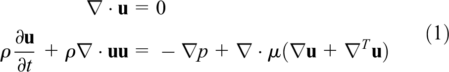
where μ, ρ, g, p, and u denote the viscosity and the density of the fluid, the gravitational acceleration, the pressure, and the velocity vector, respectively. The last term in equation (2) represents the body force due to surface tension where σ is the surface tension coefficient, κ is twice the mean curvature, and n is the unit vector normal to the interface, respectively. The surface tension acts only on the interface as indicated by the three-dimensional delta function, δ, whose arguments x and $x_{f}$ are the points at which the equation is evaluated and a point at the interface, respectively.

It is also assumed that the material properties remain constant following a fluid particle, i.e.

\frac{D ρ}{Dt} = 0; \frac{D μ}{Dt} = 0

(3)

where $\frac{D}{Dt} = \frac{\partial}{\partial t} + u \cdot \nabla$ is the material derivative. The density and viscosity vary discontinuously across the fluid interface and are given by

μ = μ_{i} I + μ_{o} (1 - I); ρ = ρ_{i} I + ρ_{o} (1 - I)

(4)

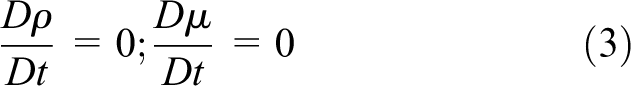
where the subscripts i and o denote the properties of the drop and bulk fluids, respectively, and I is the indicator function defined such that it is unity inside the droplet and zero outside.

The flow equations (equations (1) to (2)) are solved on a stationary staggered Eulerian grid. The spatial derivatives are approximated using second order central finite-differences for all field quantities except for the convective terms that are discretized using a third order QUICK (Quadratic Upstream Interpolation for Convective Kinematics) scheme (Leonard, 1979). Time integration is achieved using a projection method first proposed by Chorin (1968). The numerical method is briefly described here in the framework of the actual Fortran implementation. The method is explicit so that the time-step $Δ t$ is restricted for numerical stability and computed at the beginning of the time-stepping loop as

Δ t = α_{sf} min (\frac{h_{min}^{2}}{6 s_{max}}, {(\frac{h}{U})}_{min})

(5)

where $s_{max}$ is the largest value among the kinematic viscosities of the drop and ambient fluids and $h_{min}$ is the smallest grid size. $(h / U)_{min}$ is the minimum value of grid size h divided by the magnitude of the velocity U in the domain, and $α_{sf}$ is the safety factor taken as 0.9 in this study. Then the increment in velocity vector due to the convection and viscous terms is computed using the quantities evaluated at the previous time level n as

d u = {[\nabla \cdot (uu) + \frac{\nabla \cdot μ (\nabla u + \nabla^{T} u)}{ρ}]}^{n}

(6)

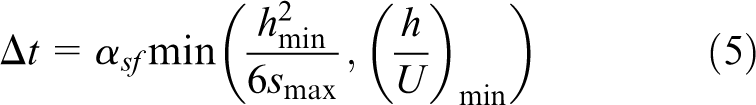
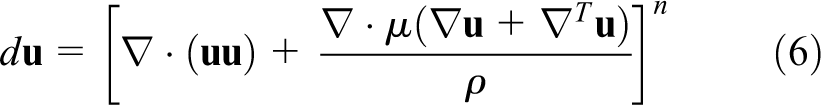
where the convective terms are evaluated using the QUICK scheme (Leonard, 1979) while the viscous terms are approximated using the central differences on the staggered grid. The body force due to surface tension forces is evaluated as

f_{f} = [\int_{A} σ κ n δ (x - x_{f}) dA]

(7)

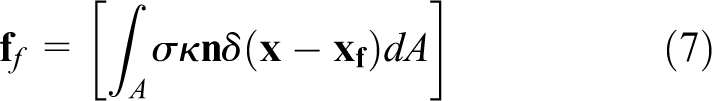
where it is first computed on the Lagrangian grid and is then distributed onto the neighboring Eulerian grid using the Peskin’s cosine distribution function as discussed in detail by Tryggvason et al. (2001). The front is then moved by a single time-step using an explicit Euler methods as

x_{f}^{n + 1} = x_{f}^{n} + u_{f}^{n} Δ t

(8)

where $u_{f}^{n}$ is the velocity interpolated onto the location of the marker point from the Eulerian grid. After this step, the body force due to surface tension forces is added to the buoyancy force and $d u$ . Then the unprojected velocity field $u^{*}$ is computed as

d u = d u + \frac{g Δ ρ^{n}}{ρ^{n}} + \frac{f_{f}}{ρ^{n}},

(9)

u^{*} = u^{n} + Δ td u

(10)

To enforce the incompressibility condition, the pressure field is computed by solving a Poisson equation in the form

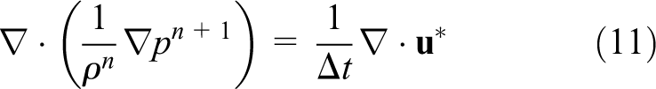
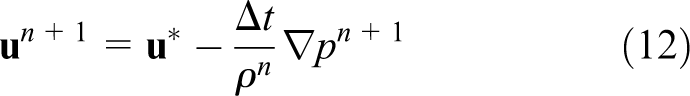
\nabla \cdot (\frac{1}{ρ^{n}} \nabla p^{n + 1}) = \frac{1}{Δ t} \nabla \cdot u^{*}

(11)

The Poisson equation (equation (11)) is solved for the pressure using the HYPRE (High Performance Preconditioners) library (HYPRE Library). Then the velocity field is corrected to satisfy the incompressibility condition as

u^{n + 1} = u^{*} - \frac{Δ t}{ρ^{n}} \nabla p^{n + 1}

(12)

Finally the indicator function is computed using the standard procedure as described by Tryggvason et al. (2001), which requires the solution of a separable Poisson equation in the form

\nabla^{2} I^{n + 1} = \nabla \cdot {(\nabla I)}^{n + 1}

(13)

which is again solved using the HYPRE libarary (HYPRE Library). To evaluate the right hand side of equation (13), unit normal vectors are first computed at the center of each front element, then distributed onto neighboring Eulerian grid points in a conservative manner, and finally the divergence is evaluated using central differences.

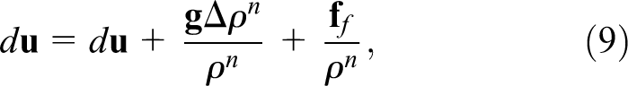
The numerical methods described above is first order accurate in time. However, second-order accuracy is recovered by using a simple predictor-corrector scheme in which the first-order solution at $n + 1$ serves as a predictor that is then corrected by the trapezoidal rule as discussed by Tryggvason et al. (2001).

In the front tracking method, the interface is used to explicitly track the fluid-fluid interface as shown in Figure 1a. The interface consists of Lagrangian points (or marker points) connected by triangular elements as shown in Figure 1b. The Lagrangian points are used to compute the surface tension forces on the interface, which are then distributed as body forces using the Peskin’s cosine distribution function (Peskin, 1977) over the neighboring Eulerian grid cells (Unverdi and Tryggvason, 1992; Tryggvason et al., 2001). The indicator function is computed at each time-step based on the location of the interface using the standard procedure (Unverdi and Tryggvason, 1992; Tryggvason et al., 2001) and is then used to set the fluid properties in each phase according to equation (4). The restructuring is performed by deleting the elements that are smaller than a pre-specified lower limit and by splitting the elements that are larger than a pre-specified upper limit in the same way as described by Tryggvason et al. (2001) to keep the element size nearly uniform. It is critically important to restructure the Lagrangian grid since it avoids unresolved wiggles due to small elements and lack of resolution due to large elements.

Figure 1.

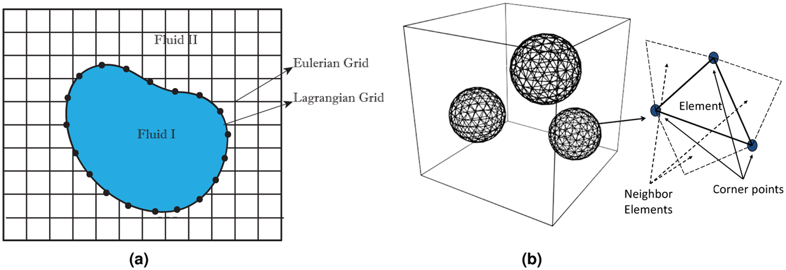
(a) Lagrangian and Eulerian grids in 2D. The flow equations are solved on the fixed Eulerian grid. The interface between different phases is represented by a Lagrangian grid consisting of connected Lagrangian points (marker points). (b) Structure of a 3D interface. Each interface is a collection of triangular elements, which have pointers to the marker points and to the adjacent elements. Marker points are the corner points of an element.

More details about the front tracking method can be found in the original paper by Unverdi and Tryggvason (1992), the review paper by Tryggvason et al. (2001) and the recent book by Tryggvason et al. (2011). See the literature for different applications of the method (Muradoglu and Tasoglu, 2010; Terashima and Tryggvason, 2010; Shin et al., 2011; Muradoglu and Tryggvason, 2014; Izbassarov and Muradoglu, 2015).

4 Parallelization of the front tracking method

In this section we present the parallelization method used for the front tracking method, particularly focusing on the parallelization of the Lagrangian grid. We first derive a data dependency graph for the equations as shown in Figure 2.

Figure 2.

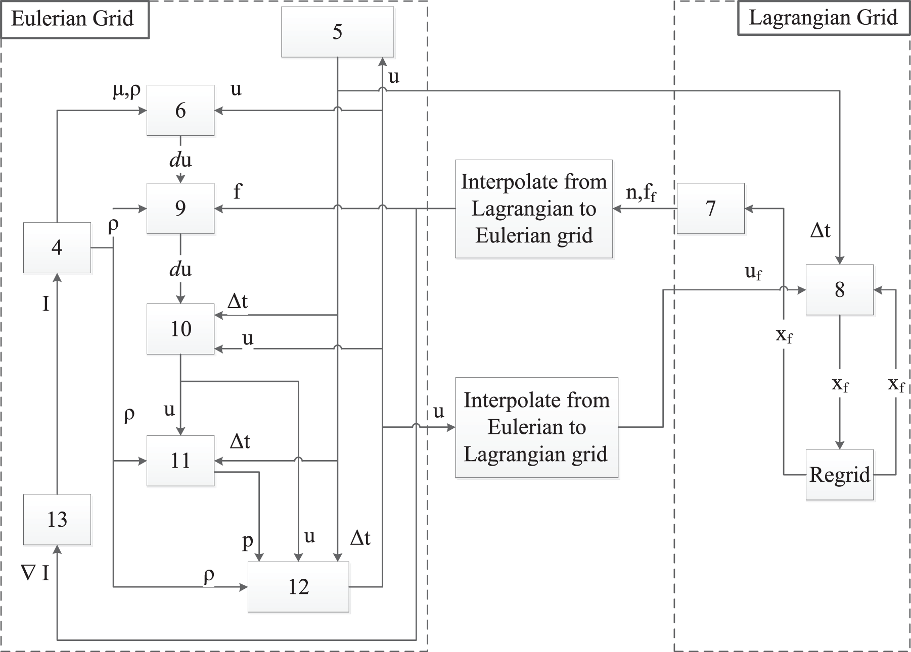
Data dependency among the tasks in the front tracking method (number inside the rectangle indicates the equation number computed in that task).

A gray rectangle in the figure represents a task and the number inside a task indicates which equation it solves. The arrows indicate data dependencies from one task (equation) to another. As Figure 2 suggests all tasks are dependent on the data from other tasks. However, the computations on the Eulerian and Lagrangian grids can be performed in parallel.

We refer to the processes computing on the Eulerian grid as Domain processes and the processes computing on the Lagrangian grid as Front. The Eulerian grid is a structured grid and as a result simple domain decomposition can be easily applied for its parallelization. Each subdomain can be assigned to one MPI-process. Similar to the Eulerian grid, we subdivide the Lagrangian grids into subgrids, and distribute bubbles among the parallel Fronts. The Front, which contains the center of a bubble becomes the owner of that bubble. Each Front is mapped to a number of Domain processes and the Front communicates with only these Domains. An example mapping of 8 Domains to 2 Fronts is shown in Figure 3a.

Figure 3.

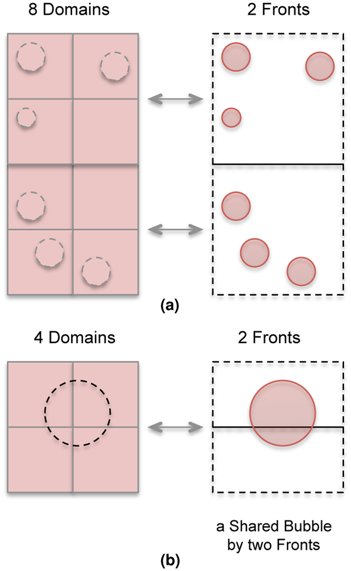
(a) Work division for parallel Fronts where upper 4 Domains are assigned to upper Front and lower 4 Domains are assigned to lower Front. (b) Two parallel Fronts with a shared bubble.

A bubble may move anywhere in the physical domain over time. There is a possibility that a bubble may be lying at the border and be shared by more than one Front as shown in Figure 3b, where a single bubble is shared by 2 Fronts. Shared bubbles complicate parallelization. To update the coordinates of the marker points that do not lie inside the owner Front are needed to be sent and received to or from other Fronts. One approach to deal with such bubbles is to break the bubble into parts and each Front works only on its own portion as discussed by Bunner (2000). This approach is computationally much more complex as it requires matching points and elements at the boundaries to maintain the data coherency. Instead we propose the following two approaches.

Owner-Computes: In this approach, the shared bubble is computed by the owner Front, which contains the center of the bubble and updates the sharers. The responsibilities of the owner include solving the equations, keeping track of the sharers, and sending or receiving the data ( $n, f_{f}$ , and $x_{f}$ ) associated with shared portion of the bubble to or from corresponding sharers. The responsibility of sharers is only to route the shared data of the bubble to the corresponding Domains.

Redundantly-All-Compute: This strategy eliminates the communication of n and $f_{f}$ among the sharers at the cost of redundantly computing a shared bubble by all the sharers. Fronts containing the shared portion of the bubble redundantly perform the computations for the shared bubble. Responsibilities of sharers include solving the equations, keeping track of new sharers, communication with their corresponding Domains, and sending or receiving the shared data $x_{f}$ to or from the sharers. The owner of the shared bubble has the same responsibilities as the sharer with an additional responsibility of sending entire data of the shared bubble to the new sharers.

We analyze these two approaches in terms of their communication overhead and present their implementation in the following sections.

5 Modeling communication

Parallelization of both the Lagrangian and Eulerian grids introduce three types of communication: (1) Front-Domain, (2) Domain-Domain, and (3) Front-Front. In this section, we analytically compute the message sizes and number of messages sent by each of the Front and Domain processes. For the sake of simplicity we assume that the Eulerian grid size is N in the x, y, and z dimensions.

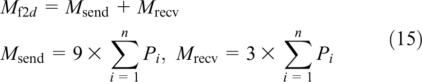
5.1 Front to domain communication

The message size in Front to Domain communication is variable as it depends on the number of bubbles, the deformation in bubbles, and the allowed distance between two points of a bubble. The total number of points in the ith bubble, $P_{i}$ , can be approximately given by

P_{i} = (π r \times \frac{N}{L} \times \frac{1}{\sqrt{a_{min} \times a_{max}})^{2}}

(14)

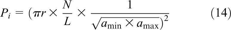
where r is the radius of the bubble and $\frac{N}{L}$ is the ratio of grid size to the length of physical domain. $a_{min}$ and $a_{max}$ are the minimum and maximum limits, respectively, for the distance allowed between two points in an element. The total message size between a Front and all its Domains in a single time-step, denoted by $M_{f 2 d}$ , can be computed by

\begin{matrix} M_{f 2 d} = M_{send} + M_{recv} \\ M_{send} = 9 \times \sum_{i = 1}^{n} P_{i}, M_{recv} = 3 \times \sum_{i = 1}^{n} P_{i} \end{matrix}

(15)

where $M_{send}$ is the data sent and $M_{recv}$ is the data received by the Front. For each point there are point coordinates in the x,y, and z directions and every point coordinate has a corresponding surface tension force and normal vector to the edge of the element. A total of 9 double precision elements per point should be sent to a Domain while only updated point coordinates (3 double precision elements) are received from a Domain. Let $d_{x}$ , $d_{y}$ , and $d_{z}$ be the geometry of the MPI processes for the Domains. For the sake of simplicity if we assume $d = d_{x} = d_{y} = d_{z}$ , then there are $d^{3}$ Domains in total. The number of messages sent and received by the Front in a single time-step would be $2 d^{3}$ because all point coordinates destined to a single Domain could be packed in a single message.

If there are f Fronts and an approximately equal number of Domains are assigned to each Front, then the number of messages and message size per Front are reduced by a factor of f; each Front exchanges $2 d^{3} / f$ messages with size of $M_{f 2 d} / f$ . However, the actual message size per Front can vary based on how bubbles are distributed in the physical domain.

5.2 Domain to domain communication

The message size in this type of communication is fixed and depends on the stationary Eulerian grid size. Every Domain needs to exchange its ghost cells (halos) with its 6 neighbors in the x, y, and z directions. Each message size is $n_{g} \times \frac{N^{2}}{d^{2}},$ , where $n_{g}$ is the depth of the ghost cells and the subdomain size is $\frac{N}{d}$ . Thus the Domain to Domain communication size, $M_{d 2 d}$ , is given by

M_{d 2 d} = 6 \times d \times N^{2} \times (n_{g} \times 14)

(16)

Each Domain needs to send at least 30 messages per time-step. The details are as follows: After receiving of n and $f_{f}$ from the Front, these values are interpolated on the Eulerian grid and needed to be updated on the neighboring Domains. As every Domain communicates with its six neighbors, a total of 6 messages are sent. Ghost cells of flow velocity, u, are communicated with all six neighboring Domains after their computation in equation (10) and equation (12), resulting in another 12 messages. Pressure and density computed in equation (11) and equation (4) result in two more message exchanges with six neighbors.

5.3 Front to front communication

Front to Front communication is required to exchange the point coordinates of the shared bubbles, which were updated by Domains. Front to Front communication is difficult to approximate as it depends on the number of the shared bubbles, the number of Fronts sharing those bubbles and the shared portion of a bubble. Let’s suppose that we have b number of shared bubbles, where each bubble is shared by s number of Fronts. The value of b depends on the total number of Fronts and the movement of bubbles during simulation. There are three types of boundaries between the Fronts as shown in Figure 4: (1) A plane boundary that is between two adjacent Fronts, (2) a line boundary where four neighboring Fronts meet, and (3) a point boundary that is shared by eight neighboring Fronts.

Figure 4.

Three types of Front boundaries: (a) plane boundary - represented by the gray plane, dividing the bubble into two parts, (b) line boundary - is the line where two planes intersect each other, and (c) point boundary - is the point where all three planes intersect.

The probability that a bubble is shared on a certain boundary depends on many variables e.g. the bubble diameter i.e. if a single large bubble is simulated it is expected to be shared on a point boundary. However, here only the probabilities of the boundary types are compared. Probabilities of boundary types are based on the amount of space they occupy in the domain. For example, if a domain is divided into 8 subdomains, then there will be only single point boundary, two line boundaries, and three plane boundaries. If there are 100 bubbles then at maximum only one bubble can be shared on the point boundary. On the other hand, bubbles shared on the lines are more probable than points and the maximum probability is to be shared on a plane boundary. Moreover the many bubble case is considered here so the diameters of the bubbles are expected to be smaller when compared to the domain size. Thus it is more likely that a bubble will be shared on a plane boundary compared to a line or point. As a result, the value of s for a large number of shared bubbles is 2.

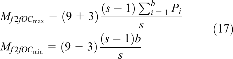
5.3.1 Owner-computes the shared bubble strategy

In the owner-computes strategy the owner of the bubble sends point coordinates, corresponding surface tension force, and normal vector to the sharers and then receives the updated point coordinates from them. The amount of shared points is initially small when a bubble becomes shared and increases as the bubble moves. The amount of shared points starts decreasing when a bubble’s center crosses the boundary and the ownership is transferred to the neighboring Front. In one extreme case (when the center of the bubble is almost at the boundary) the fraction of points in the owner Front will be slightly more than half, quarter, and one eighth of total points for plane, line, and point boundaries, respectively. Thus, $\frac{(s - 1)}{s}$ fraction of the points are exchanged with sharers. In another extreme case, only 1 point from each shared bubble is exchanged. Then, the number of messages exchanged per time-step is $2 (s - 1) b$ . The minimum and maximum communication size is denoted by $M_{f 2 fO C_{\min}}$ and $M_{f 2 fO C_{\max}}$ , respectively, for both sending and receiving the point coordinates per time-step driven from equation (15) for all the Fronts are represented by

\begin{matrix} M_{f 2 fO C_{max}} = (9 + 3) \frac{(s - 1) \sum_{i = 1}^{b} P_{i}}{s} \\ M_{f 2 fO C_{min}} = (9 + 3) \frac{(s - 1) b}{s} \end{matrix}

(17)

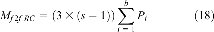
5.3.2 Redundantly-all-compute the shared bubble strategy

Communication in the redundantly-all-compute strategy is different when compared to the owner-computes strategy because communication has to take place among all the Fronts sharing the bubble and each Front has to redundantly send the same point coordinates that were updated in Front to all the other sharers. The number of messages exchanged per time-step is $s (s - 1) b$ . The communication size per time-step for all the Fronts, $M_{f 2 fRC}$ , is given by

M_{f 2 f RC} = (3 \times (s - 1)) \sum_{i = 1}^{b} P_{i}

(18)

5.4 Comparison of communication overheads

Table 1 summarizes the communication overhead for all three types of communication. The number of Domain processes $(d^{3})$ and bubbles $(n)$ are dominant factors in the communication overhead. In the simulation the number of shared bubbles, b, is typically much smaller than the total number of bubbles. Similarly, the number of sharers is smaller than the number of fronts, f or domains, $d^{3}$ . As a result, it is expected that the communication size in Domain to Domain is much larger than Front to Domain, which is also larger than the Front to Front communication. The number of messages is expected to be the highest for Domain to Domain. In Front to Front, the number of messages mainly depends on how many bubbles are shared and the number of sharers.

Table 1.

Number of messages and message sizes for different types of communication with the assumption of uniform distribution of bubbles.

Communication type	Number of messages	Communication size
Front to Domain	$2 d^{3}$	$M_{f 2 d} = (9 + 3) \sum_{i = 1}^{n} P_{i}$
Domain to Domain	$30 d^{3}$	$M_{d 2 d} = 6 \times d \times N^{2} \times (n_{g} \times 14)$
Front to Front
(Owner-computes)	$2 (s - 1) b$	$M_{f 2 fO C_{max}} = (9 + 3) \frac{(s - 1) \sum_{i = 1}^{b} P_{i}}{s}$
(Redundantly-all-compute)	$s (s - 1) b$	$M_{f 2 fRC} = (3 \times (s - 1)) \sum_{i = 1}^{b} P_{i}$

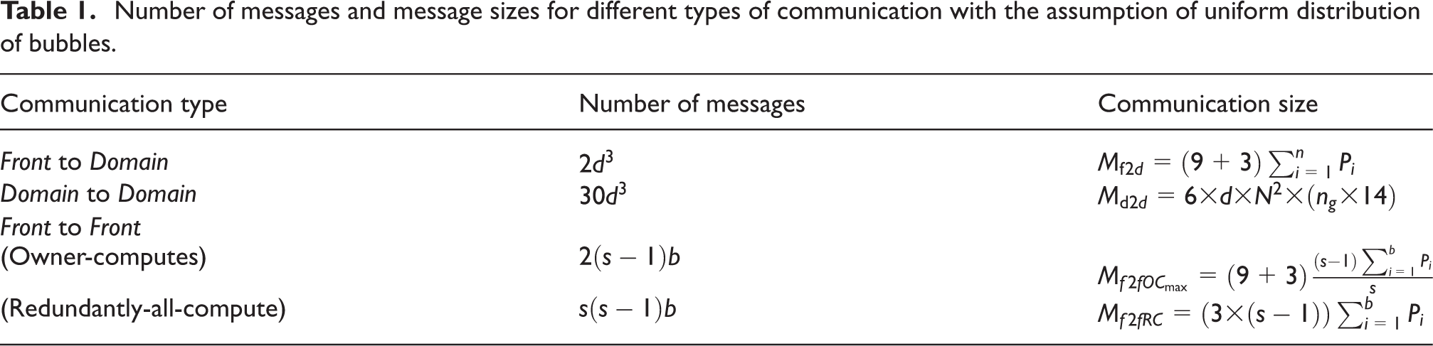
The cost model for the redundantly-all-compute strategy holds at all times because the model is independent of what portion of a bubble is shared. On the contrary we can only approximate the communication cost of the owner-computes strategy. If we take the average of the minimum and maximum communication size into account for owner-computes, then the following observations can be made.

If a bubble is shared at a plane boundary or line boundary, then redundantly-all-compute is advantageous in terms of communication size; owner-computes strategy would exchange 3b and 9b more double precision elements, for planes and lines respectively.

If a bubble is shared at a point boundary, then owner-compute is advantageous in terms of communication size because there are eight sharers.

The number of messages for both strategies are equal when a bubble is shared on a plane boundary but the redundantly-all-compute strategy exchanges more messages when a bubble is shared on a line or a point boundary.

Considering that it is more likely for bubbles to be shared at a plane or line boundary, redundantly-all-compute should perform better because of its smaller overall communication volume. On the other hand, redundantly-all-compute comes at the expense of increased computation at the sharer Fronts.

Based on these observations, there is no clear winner. The best strategy depends on how the bubbles are shared, the balance between the interconnection network and compute capabilities of the underlying machine, and finally how much communication overhead is hidden behind computation. As a result, it is worthwhile to implement both strategies and explore their actual performance.

6 Implementation

The Eulerian grid is partitioned in all three dimensions of space resulting in a number of subgrids (Domains), each of which is executed by a separate MPI process. Every Domain works on its portion of the stationary Eulerian grid while exchanging boundary values with neighboring Domains. The Domain processes are responsible for solving the equations on the Eulerian grid indicated in Figure 2. The Poisson equation for the pressure (equation (11)), and the indicator function (equation (13)) are solved using the HYPRE library (HYPRE Library).

The interpolation of n and $f_{f}$ from the Lagrangian to Eulerian grid and the interpolation of u from the Eulerian to Lagrangian grid mentioned in Figure 2 can be done either in the Domain or in the Front processes. Both these interpolations are done in the Domain to reduce the communication size because the Eulerian grid is denser than the Lagrangian grid. We send $x_{f}$ from the Front to the Domain because it is needed for interpolation. The Domain process also solves equation (8) as it simply updates $x_{f}$ .

In the remainder of this section we present the implementation details for the two parallelization strategies for the Lagrangian grid. It is important to note that we use non-blocking communication calls as much as possible as a result some of the communication cost might be hidden behind computation.

6.1 Parallel front with owner-computes shared bubbles

The design for the parallel Front using the owner-computes strategy is shown in Figure 5a. The inner do-loop executes twice for each time-step to achieve second order accuracy in time. A bubble created initially inside a Front may also be shared with another Front or it may become shared in any time-step. We implement the Find_Shared_Interface subroutine, which iterates over all bubbles and finds the bubbles that are shared among multiple Fronts. 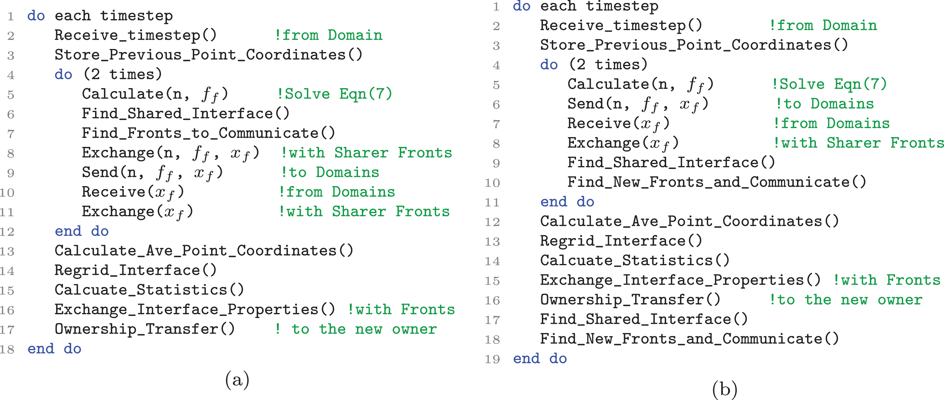The next step is to send and receive the n and $f_{f}$ at the shared point coordinates along with $x_{f}$ to and from the sharers.

Figure 5.

(a) Parallel Front design of owner-computes strategy for the shared bubble. (b) Parallel Front design of redundantly-all-compute strategy for the shared bubble.

Instead of all Fronts communicating with each other we optimize the communication overhead by adding the Find_Fronts_to_Communicate subroutine, which finds and notifies only those Fronts that need to communicate with each other. In this subroutine each Front fills an array, having length equal to the number of Fronts, with a flag to indicate whether it needs to communicate with a specific Front or not. A communication table at each Front process is built using this array and serves as an input to the MPI_AllGather. Based on this communication table all owners exchange $n, f_{f}$ , and $x_{f}$ with sharers in the Exchange $(n, f_{f}, x_{f})$ subroutine and then all Fronts communicate with their corresponding Domains. After receiving the updated point coordinates $x_{f}$ from Domains, sharers in the Exchange $(x_{f})$ subroutine send these updated point coordinates to the owners.

In the Exchange_Interface_Properties subroutine a single Front gather Interface_Properties for all bubbles from their owners and then broadcasts these to all Fronts. At the end of a time-step if the center of the bubble has moved from the owner Front to some other Front then the ownership is transferred to the new Front. When that happens, the Ownership_Transfer subroutine sends all the point coordinates, element corners, neighbors, and surface tension data to the new owner.

6.2 Parallel front with redundantly-all-compute shared bubbles

Figure 5b shows the design for the redundantly-all-compute strategy. During the initialization every Front performs additional work to find the shared bubbles and notifies the sharers to redundantly create that bubble. After creating the shared bubbles redundantly each Front calculates surface tension force and normal vectors at the corresponding point coordinates and sends them to their allocated Domains. After receiving the updated point coordinates $x_{f}$ from the Domains, each Front in the Exchange $(x_{f})$ subroutine send its received portion of the point coordinates to all other sharers so that every Front can have all the relevant point coordinates for the shared bubbles.

As a result of the point coordinate update and movement of a bubble, some portion of a bubble may now be shared with a new Front that was previously not computing the bubble. The Find_Shared_Interface subroutine is called to find the shared bubbles and their sharers. Subsequently in the Find_New_Fronts_and_Communicate subroutine the owner of the bubbles finds the new sharers and sends them all the point coordinates, old point coordinates, element corners, neighbors, and surface tension so that these new sharers can redundantly start computing the shared bubble. Exchange_Interface_Properties works similar to the one in the owner-computes strategy. However, in the Ownership_Transfer subroutine sending a bubble’s data is eliminated because all the Fronts sharing the bubble have already computed that information. Lastly, because averaging and regridding subroutines may introduce new sharers, Find_Shared_Interface and Find_New_Fronts_and_Communicate functions are called again to discover new sharers.

7 Results and discussion

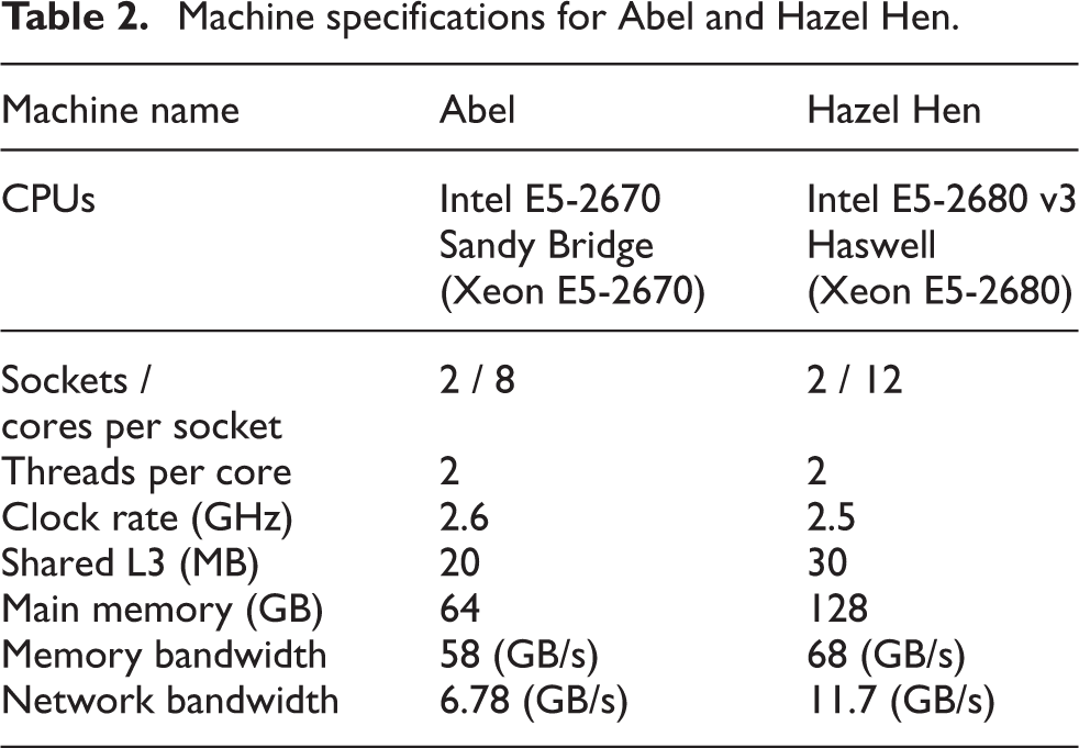
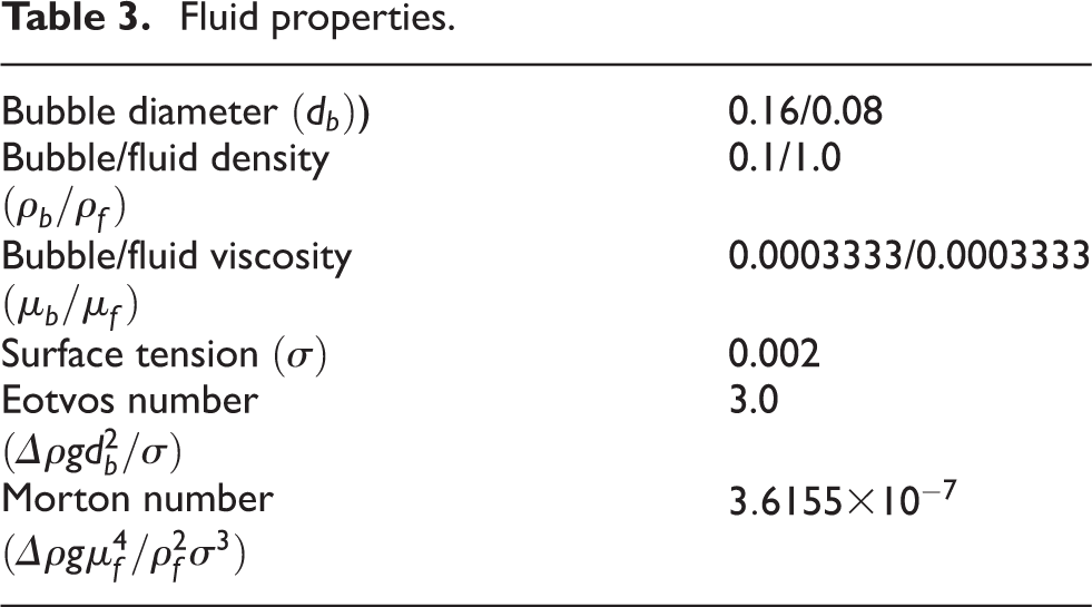
We carry out the performance studies for the parallel front tracking method on two supercomputers. The first one is the Abel cluster located at the University of Oslo and other is the Hazel Hen located at the High Performance Computing Centre, Stuttgart. Specifications of both Abel and Hazel Hen are listed in Table 2. Abel has an FDR (Fourteen Data Rate) Infiniband interconnection network while Hazel Hen has a Cray Aries Dragonfly network. Throughout the performance studies we use 0.058 void fraction and deformable bubbles with fluid properties given in Table 3. Fluid properties are mainly based on the deformable bubble case used by Lu and Tryggvason (2008) and the bubble’s diameter is selected so that a bubble can have a reasonable number of grid points i.e. 28 in this case. We use periodic boundary conditions for all directions and double precision arithmetic in our calculations. In our experiments we found that shared memory parallelism do not perform well as compared to distributed memory parallelism. Using hyper-threading within MPI processes produces optimal performance. This conclusion is aligned with prior work by Reguly et al. (2016). All our experiments use 2 OpenMP (Open Multi-Processing) threads for hyper-threading within each MPI process.

Table 2.

Machine specifications for Abel and Hazel Hen.

Machine name	Abel	Hazel Hen
CPUs	Intel E5-2670	Intel E5-2680 v3
	Sandy Bridge (Xeon E5-2670)	Haswell (Xeon E5-2680)
Sockets /	2 / 8	2 / 12
cores per socket
Threads per core	2	2
Clock rate (GHz)	2.6	2.5
Shared L3 (MB)	20	30
Main memory (GB)	64	128
Memory bandwidth	58 (GB/s)	68 (GB/s)
Network bandwidth	6.78 (GB/s)	11.7 (GB/s)

Table 3.

Fluid properties.

Bubble diameter $(d_{b})$ )	0.16/0.08
Bubble/fluid density	0.1/1.0
$(ρ_{b} / ρ_{f})$
Bubble/fluid viscosity	0.0003333/0.0003333
$(μ_{b} / μ_{f})$
Surface tension $(σ)$	0.002
Eotvos number	3.0
$(Δ ρ {gd}_{b}^{2} / σ)$
Morton number	$3.6155 \times 10^{- 7}$
$(Δ ρ g μ_{f}^{4} / ρ_{f}^{2} σ^{3})$

7.1 Strong scaling

Strong scaling studies enable us to observe the behavior of the code for solving the same problem with more resources. Grid parameters and different input configurations for strong scaling runs are given in Table 4. Domain size is the container size that we are simulating and the mesh resolution is the Eulerian grid that is used in the Domain. The baseline for the speedup is the redundantly-all-compute strategy with two MPI processes one for the Domain and one for the Front.

Table 4.

Strong scaling inputs.

Domain size (x, y, and z)	2 × 2 × 2
Mesh resolution	256 × 256 × 256 (Abel) /
	512 × 512 × 512 (Hazel Hen)
Number of bubbles	216 (Abel) / 1728 (Hazel Hen)
Number of processes (x,y,z) =	2 = 1 × 1 × 1 + 1 × 1 × 1
Domain process geometry +	4 = 2 × 1 × 1 + 2 × 1 × 1
Front process geometry	8 = 2 × 2 × 1 + 2 × 2 × 1
	16 = 2 × 2 × 2 + 2 × 2 × 2
	32 = 4 × 2 × 2 + 4 × 2 × 2
	64 = 4 × 4 × 2 + 4 × 4 × 2
	128 = 4 × 4 × 4 + 4 × 4 × 4
	256 = 8 × 4 × 4 + 8 × 4 × 4
	512 = 8 × 8 × 4 + 8 × 8 × 4
MPI processes/node	16 (Abel) / 24 (Hazel Hen)

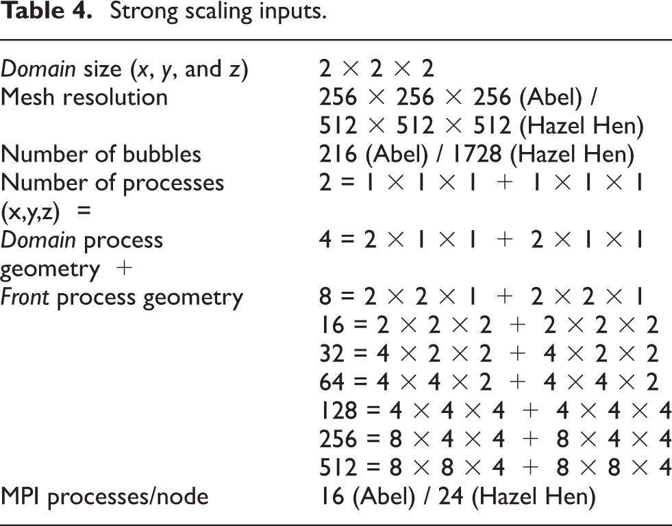
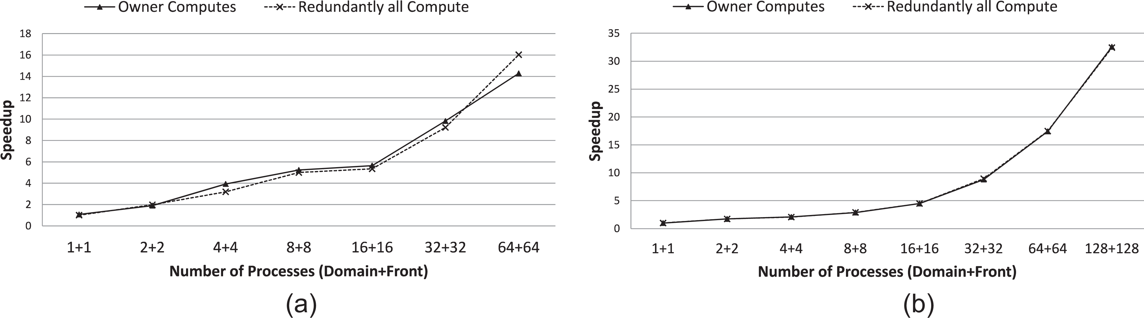
Figure 6 shows the results for the strong scaling. On Abel, for the given mesh size $(256^{3})$ , the best speedup for both strategies is achieved when 64 Domain+64 Front processes are used. The speedup over the baseline with 1+1 processes is 16× for redundantly-all-compute and 14x for the owner-computes strategy. Increasing the MPI processes beyond 128 is not realistic because at that point there are only few data points assigned to each MPI process. On Hazel Hen, we achieve much better scalability because Hazel Hen has a higher network bandwidth, which is 11.7 GB/s, almost twice of that of Abel. The maximum speedup we achieve on Hazel Hen is around 32.5× over 1+1 processes for both strategies. Again here increasing the MPI processes beyond 256 is not realistic.

Figure 6.

Strong scaling speedup (higher is better). (a) Abel. (b) Hazel Hen.

When we compare two parallelization strategies of the Lagrangian grid, the redundantly-all-compute strategy performs better than the owner-computes strategy when the number of processes are large. This is because increasing the number of processes results in more subdomains, thus more boundaries ultimately increasing the number of shared bubbles. For fewer number of processes owner-computes performs better because the communication overhead due to shared bubbles is lower than the extra computation performed by the redundantly-all-compute strategy. These results are in line with our conclusions in communication modeling i.e. the communication overhead due to shared bubble is lower for redundantly-all-compute strategy at the expense of extra computation. The performance gap between the two strategies is small, not visible in the figure, on Hazel Hen as compared to Abel due to the fast interconnection network on Hazel Hen.

7.2 Weak scaling

We conduct a weak scaling study for the front tracking method because high mesh resolutions allow researchers to investigate complex fluid-fluid or fluid-gas interaction problems. Inputs for weak scaling are shown in Table 5. In this study, we fix the amount of computational work assigned to each process in all six inputs: $64 \times 128 \times 128$ grid size to each Domain process and approximately 14 bubbles to each Front process.

Table 5.

Weak scaling inputs.

	Input-1/2/3/4/5/6
Domain size (x, y, z)	2 × 4 × 4/4 × 4 × 4/
	4 × 8 × 4/4 × 8 × 8/
	8 × 8 × 8/8 × 8 × 16
Mesh resolution	256 × 512 × 512/
	512 × 512 × 512/
	512 × 1024 × 512/
	512 × 1024 × 1024/
	1024 × 1024 × 1024/
	1024 × 1024 × 2048
Number of bubbles	864/1728/3456/
	6912/13,824/27,648
Number of processes (x, y, z) =	128 = 4 × 4 × 4 + 4 × 4 × 4/
Domain process geometry +	256 = 8 × 4 × 4 + 8 × 4 × 4/
Front process geometry	512 = 8 × 8 × 4 + 8 × 8 × 4/
	1024 = 8 × 8 × 8 + 8 × 8 × 8
	2048 = 8 × 8 × 16 + 8 × 8 × 16
	4096 = 8 × 16 × 16 + 8 × 16 × 16
MPI processes/node	16 (Abel) / 24 (Hazel Hen)

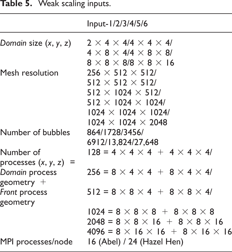
Results for weak scaling are shown in Figure 7. Although the computational work per process stays the same, the time per iteration slowly rises as we scale due to the communication overhead on Abel. On the other hand, both strategies show good scaling on Hazel Hen up to 2048 processes (1024+1024) but time per iteration rises with further increase in the number of processes. Although the number of messages and communication size per process stay the same, the total number of messages and message sizes increase in all three types of communication that leads to network contention. In the implementation we use global synchronizations such as MPI_AllReduce to select the minimum time-step value, MPI_AllGather to assemble the communication matrix in the Front processes, and MPI_Broadcast to send the interface properties to the Front processes. These global synchronizations lower the parallel efficiency beyond 2048 processes. Future work will further improve the communication and synchronization costs by removing some of the global synchronization points.

Figure 7.

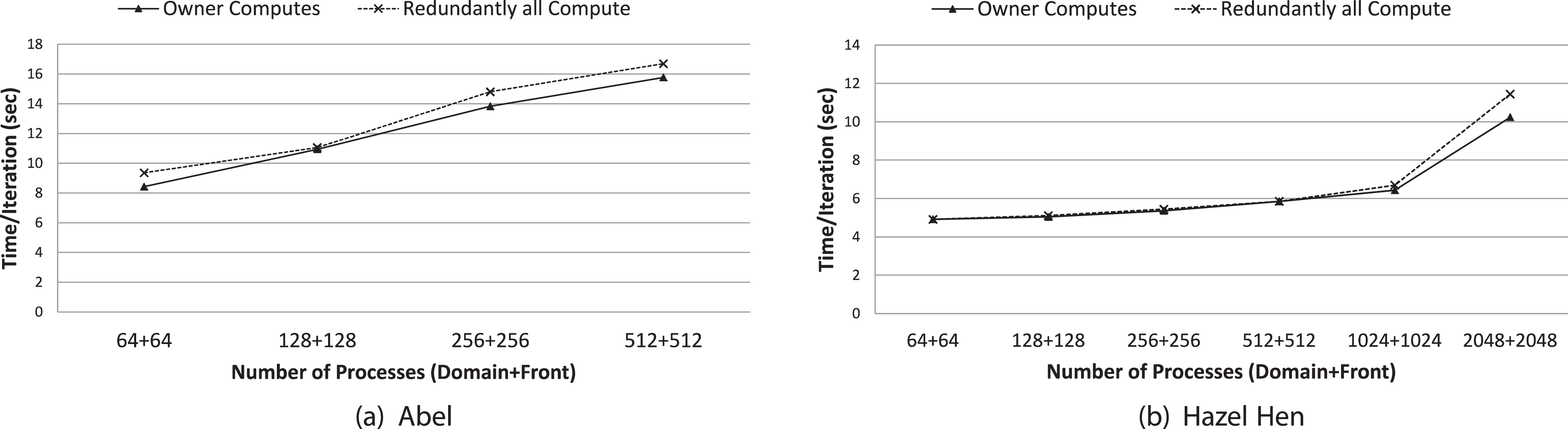
Weak scaling (lower is better).

7.3 Process placement and ratios

We also compare two placement scenarios for the Domain and Front processes. In the first scenario, ‘co-located’, Domains and their corresponding Fronts are placed in the same compute node while in the second scenario, ‘separated’, Domains and Fronts processes are placed in separate compute nodes. For example, consider the case of 8 (4+4), where processes numbered 0–3 are the Domain processes and 4–7 are the Front processes. In the separated scenario we schedule the processes 0–3 to run on the first node and 4–7 on the second node. In the co-located scenario processes 0,2,4,6 are scheduled to run on the first node and 1,3,5,7 on the second node. Note that in both scenarios the same number of resources (cores and nodes) are used to schedule MPI processes. We use “cyclic:cyclic” for co-located and “block:block” for separated in the Slurm (SLURM) task distribution method in the job submission script. As shown in Figure 8 placing Fronts and their corresponding Domains in separated nodes performs better than co-locating them in the same node. The performance improvement becomes clearer as the number of processes is increased. Indeed our communication model suggests that the separated task distribution should perform better because the Domain to Domain communication plus Front to Front communication is more than the Front to Domain communication. For example, consider the (32+32) case. Based on equations (15) to (17), in a single time-step, Domain to Domain communication results in 36.7 MB of data exchange in 960 messages, Front to Front communication results in 5.77 MB of data exchange using 216 messages, and finally Front to Domain communication results in 34.6 MB of data exchange in 64 messages. As a result, placing these two types of processes on different nodes is the best since node to node communication is more costly than within the node communication.

Figure 8.

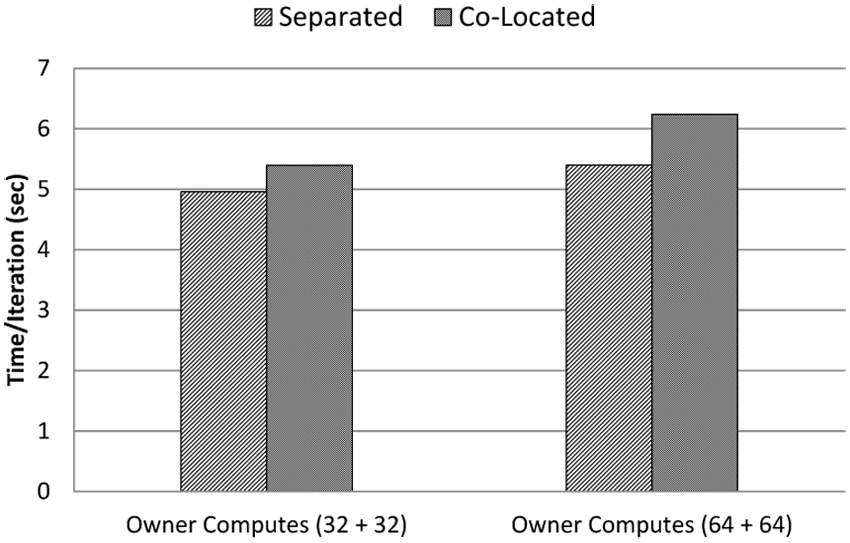
Co-located vs separated Domain and corresponding Front (lower is better).

In Figure 6 we ran the application by assigning one Front to every Domain. Next, we experiment with different Domain to Front ratios to find an optimal value. The ratio between Domain and Front processes should be balanced to avoid underutilization of resources. Computation performed by a Front process is considerably less expensive than a Domain process. Thus sparing more processes for Front than Domain is not beneficial. The result shown in Figure 9 suggests that assigning a single Front to every 4 Domains can achieve almost the same speedup as single Front to single Domain. 2:1 ratio (two Domains for every Front) performs slightly better in some cases, however in strong and weak scaling we did not observe any significant gain for 2:1 ratio over 1:1 because the benefit of additional resources is negated by the additional communication overhead. Although the figure shows only the owner-computes strategy, the Domain to Front ratios for both strategies give similar performance.

Figure 9.

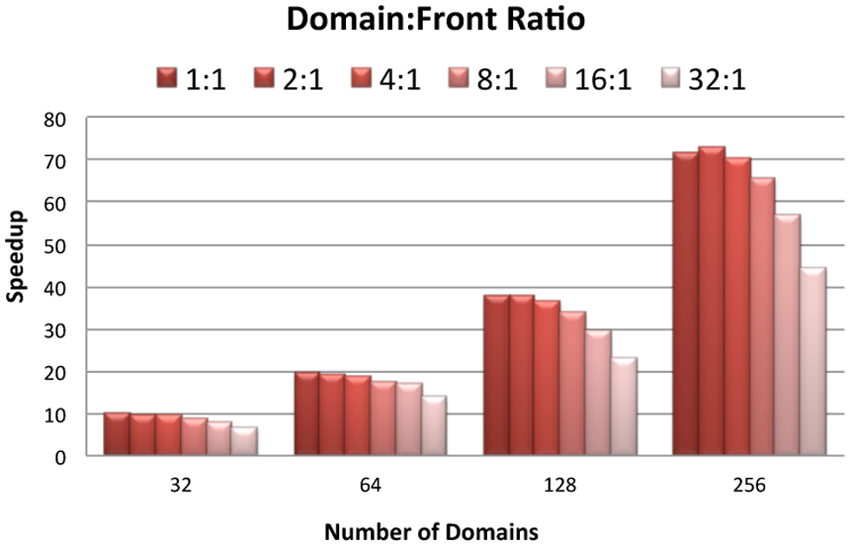
Number of Domains to number of Fronts ratio (higher is better).

8 Conclusions

Eulerian–Lagrangian methods for multiphase flows simulations are more challenging than Eulerian methods to parallelize because the Lagrangian grid is unstructured, movable, and restructures continuously with time and requires coupling with the Eulerian grid. In this work, we focused on the parallelization of the front tracking method that belongs to the family of the Eulerian–Lagrangian approach. The parallelization of the method is necessary to be able to simulate large number of interfaces (bubbles) and to overcome the memory limitation on a single compute node. We implemented and analyzed two different parallelization strategies for the Lagrangian grid, namely owner-computes and redundantly-all-compute. The communication cost model we devised for these parallelization strategies suggests that the best performing strategy depends on the distribution of bubbles in the fluid and the underlying machine specifications.

Our implementation can achieve 32.5x speedup on 256 cores on the Hazel Hen supercomputer and 16x speedup on the Abel supercomputer with 128 cores over the baseline (2 cores) with strong scaling. We conducted the weak scaling study of our code by simulating up to 28 thousand bubbles on $1024 \times 1024 \times 2048$ grid size using about four thousand cores, and achieved very good scaling. The experimental results indicate that owner-computes slightly performs better on weak scaling studies but redundantly-all compute performs better in strong scaling studies. Thus, we expect that on a machine with high compute capability but low network bandwidth, redundantly-all-compute is likely to outperform owner-computes. Finally co-locating Domain processes on the same node performs better than splitting a node between Domain and its corresponding Front processes because the Domain to Domain communication size is significantly more than the Front to Domain communication.

Footnotes

Acknowledgements

We acknowledge PRACE for awarding us access to the Hazel Hen supercomputer in Germany. Lastly we thank Xing Cai from Simula Research Laboratory for his input.

Declaration of Conflicting Interests

The author(s) declared no potential conflicts of interest with respect to the research, authorship, and/or publication of this article.

Funding

The author(s) disclosed receipt of the following financial support for the research, authorship, and/or publication of this article: Authors from the Department of Computer Engineering at Koç University is supported by the Scientific and Technological Research Council of Turkey (TUBITAK), Grant No. 215E193. Authors from the Department of Mechanical Engineering at Koç University is supported by TUBITAK, Grant No. 115M688. We acknowledge PRACE for awarding us access to the Hazel Hen supercomputer in Germany. Lastly we thank Xing Cai from Simula Research Laboratory for his input.

References

Aggarwal

Gada

Sharma

(2013) Parallelization methodology and performance study for level set method based simulation of a 3-D transient two-phase flow. Numerical Heat Transfer, Part B: Fundamentals 63: 327–356.

Alfonsi

Ciliberti

Mancini

. (2014) GPGPU implementation of mixed spectral-finite difference computational code for the numerical integration of the three-dimensional time-dependent incompressible Navier–Stokes equations. Computers & Fluids 102: 237–249.

Ang

Barrett

Benner

. (2014) Abstract machine models and proxy architectures for exascale computing. In: Hardware-Software Co-Design for High Performance Computing, New Orleans, LA, November 2014, pp. 25–32.

Bunner

(2000) Large scale simulations of bubbly flow. PhD Thesis, University of Michigan, USA.

Bunner

Tryggvason

(2002a) Dynamics of homogeneous bubbly flows. Part 1. Rise velocity and microstructure of the bubbles. Journal of Fluid Mechanics 466: 17–52.

Bunner

Tryggvason

(2002b) Dynamics of homogeneous bubbly flows. Part 2. Velocity fluctuations. Journal of Fluid Mechanics 466: 53–84.

Center of Applied Scientific Computing, Lawrence Livermore National Laboratory. HYPRE Library, http://computation.llnl.gov/project/linear_solvers/software.php (2006, accessed 21 April 2016).

Chorin

(1968) Numerical solution of the Navier–Stokes equations. Mathematics of Computation 22: 745–762.

Darmana

Deen

Kuipers

JAM

(2006) Parallelization of an Euler–Lagrange model using mixed domain decomposition and a mirror domain technique: Application to dispersed gas-liquid two-phase flow. Journal of Computational Physics 220: 216–248.

10.

Deckwer

(1992) Bubble Column Reactors. United Kingdom: John Wiley and Sons Ltd.

11.

Demmel

(2013) Communication-avoiding algorithms for linear algebra and beyond. In: IEEE 27th international symposium on parallel and distributed processing (IPDPS2013), Boston, MA, 20–24 May 2013, pp.585–585. IEEE Xplore, IEEE.

12.

Driscoll

Georganas

Koanantakool

. (2013) A communication-optimal N-body algorithm for direct interactions. In: IEEE 27th international symposium on parallel and distributed processing (IPDPS2013), Boston, MA, 20–24 May 2013, pp.1075–1084. IEEE Xplore, IEEE.

13.

Esmaeeli

Tryggvason

(1996) An inverse energy cascade in two-dimensional, low Reynolds number bubbly flows. Journal of Fluid Mechanics 314: 315–330.

14.

Fix

Glimm

. (2005) A TSTT integrated frontier code and its applications in computational fluid physics. Journal of Physics: Conference Series 16: 471–475.

15.

Furusaki

Fan

Garside

(2001) The Expanding World of Chemical Engineering. 2nd ed. London: Taylor and Francis.

16.

George

Warren

(2002) A parallel 3D dendritic growth simulator using the phase-field method. Journal of Computational Physics 177: 264–283.

17.

Glimm

Grove

. (2000) Robust computational algorithms for dynamic interface tracking in three dimensions. SIAM Journal on Scientific Computing 21(6): 2240–2256.

18.

Glimm

Grove

. (2001) A critical analysis of Rayleigh–Taylor growth rates. Journal of Computational Physics 169: 652–677.

19.

Glimm

Grove

Lindquist

. (1988) The bifurcation of tracked scalar waves. SIAM Journal on Scientific and Statistical Computing 9(1): 61–79.

20.

Glimm

Grove

Zhang

(2002) Interface tracking for axisymmetric flows. SIAM Journal on Scientific Computing 24: 208–236.

21.

Intel Corporation. Intel Xeon Processor E5-2670, http://ark.intel.com/products/64595/Intel-Xeon-Processor-E5-2670-20M-Cache-2_60-GHz-8_00-GTs-Intel-QPI (2012, accessed 9 January 2017).

22.

Intel Corporation. Intel Xeon Processor E5-2680 v3, http://ark.intel.com/products/81908/Intel-Xeon-Processor-E5-2680-v3-30M-Cache-2_50-GHz (2014, accessed 9 January 2017).

23.

Izbassarov

Muradoglu

(2015) A front-tracking method for computational modeling of viscoelastic two-phase systems. Journal of Non-Newtonian Fluid Mechanics 223: 122–140.

24.

Kuan

Sim

Hassan

. (2013) Parallel Eulerian–Lagrangian method with adaptive mesh refinement for moving boundary computation. In: 51st AIAA aerospace sciences meeting including the new horizons forum and aerospace exposition, aerospace sciences meetings, Grapevine, USA, 7–11 January 2013, paper no. AIAA 2013-0370, pp. 1–23. Reston, VA, USA: American Institute of Aeronautics and Astronautics.

25.

Leonard

(1979) A stable and accurate convective modelling procedure based on quadratic upstream interpolation. Computer Methods in Applied Mechanics and Engineering 19(1): 59–98.

26.

(1993) Study of three-dimensional Rayleigh–Taylor instability in compressible fluids through level set method and parallel computation. Physics of Fluids 5: 1904–1913.

27.

Tryggvason

(2008) Effect of bubble deformability in turbulent bubbly upflow in a vertical channel. Physics of Fluids 20: (040701-1)–(040701-6).

28.

Muradoglu

Tasoglu

(2010) A front tracking method for computational modeling of impact and spreading of viscous droplets on solid walls. Computers & Fluids 39(4): 615–625.

29.

Muradoglu

Tryggvason

(2014) Simulations of soluble surfactants in 3D multiphase flow. Journal of Computational Physics 274: 737–757.

30.

Nkonga

Charrier

(2002) Generalized parcel method for dispersed spray and message passing strategy on unstructured meshes. Parallel Computing 28: 369–398.

31.

Peskin

(1977) Numerical analysis of blood flow in the heart. Journal of Computational Physics 25: 220–252.

32.

Reddy

Banerjee

(2015) GPU accelerated VOF based multiphase flow solver and its application to sprays. Computers & Fluids 117: 287–303.

33.

Reguly

Mudalige

Bertolli

. (2016) Acceleration of a full-scale industrial CFD application with OP2. IEEE Transactions on Parallel and Distributed Systems 27(5): 1265–1278.

34.

Shin

Yoon

Juric

(2011) The local front reconstruction method for direct simulation of two- and three-dimensional multiphase flows. Journal of Computational Physics 230(17): 6605–6646.

35.

Auble

Bartkiewicz

Christiansen

. (2013, accessed 20 February 2017).

36.

Terashima

Tryggvason

(2010) A front tracking method with projected interface conditions for compressible multi-fluid flows. Computers & Fluids 39(10): 1804–1814.

37.

Tryggvason

Bunner

Esmaeeli

. (2001) A front tracking method for the computations of multiphase flow. Journal of Computational Physics 169: 708–759.

38.

Tryggvason

Scardovelli

Zaleski

(2011) Direct Numerical Simulations of Gas-Liquid Multiphase Flows. Cambridge, UK: Cambridge University Press.

39.

Unat

Chan

Zhang

. (2015) Exasat: An exascale co-design tool for performance modeling. International Journal of High Performance Computing Applications 29(2): 209–232.

40.

Unverdi

Tryggvason

(1992) A front-tracking method for viscous, incompressible, multi-fluid flows. Journal of Computational Physics 100: 25–37.

41.

Wang

Chang

Kale

. (2006) Parallelization of a level set method for simulating dendritic growth. Journal of Parallel and Distributed Computing 66: 1379–1386.

42.

You

Demmel

Czechowski

. (2015) CA-SVM: Communication-avoiding support vector machines on distributed systems. In: IEEE 29th international symposium on parallel and distributed processing (IPDPS2015), Hyderabad, India, 25–29 May 2015, pp.847–859. IEEE Xplore, IEEE.