The ELAPS framework: Experimental Linear Algebra Performance Studies

Abstract

In scientific computing, optimal use of computing resources comes at the cost of extensive coding, tuning, and benchmarking. While the classic approach of “features first, performance later” is supported by a variety of tools such as Tau, Vampir, and Scalasca, the emerging performance-centric approach, in which both features and performance are primary objectives, is still lacking suitable development tools. For dense linear algebra applications, we fill this gap with the Experimental Linear Algebra Performance Studies (ELAPS) framework, a multi-platform open-source environment for easy, fast, and yet powerful performance experimentation and prototyping. In contrast to many existing tools, ELAPS targets the beginning of the development process, assisting application developers in both algorithmic and optimization decisions. With ELAPS, users construct experiments to investigate how performance and efficiency depend on factors such as caching, algorithmic parameters, problem size, and parallelism. Experiments are designed either through Python scripts or a specialized Graphical User Interface (GUI), and run on a spectrum of architectures, ranging from laptops to accelerators and clusters. The resulting reports provide various metrics and statistics that can be analyzed both numerically and visually. In this article, we introduce ELAPS and illustrate its practical value in guiding critical performance decisions already in early development stages.

Keywords

Performance dense linear algebra experimentation algorithm selection performance prediction

1. Introduction

The field of high-performance computing is largely concerned with optimal resource utilization. Since performance depends on the choice of algorithms, parameters, libraries, and even computing environment, maximizing efficiency is a task that comes at the cost of extensive coding, tuning, and benchmarking. Many existing tools—an overview is provided in the following—are designed to assist developers in analyzing existing codes, exposing hot spots, bottlenecks, communication patterns, and other possible causes for low efficiency and/or scalability. To instead support dense linear algebra developers in performance-related decisions right from the early stages of development—even before the actual coding—we propose a rich and flexible environment for rapid algorithm and performance experimentation.

The Experimental Linear Algebra Performance Studies (ELAPS) framework allows users to create “experiments” to explore multiple algorithms and algorithmic variants, to test different parallelization strategies, to compare alternative libraries, to investigate the impact of caching, and to tune algorithmic parameters. Experiments are built by combining one or more constructs commonly encountered in linear algebra computations, and are specified either through Python scripts or a specialized and intuitive Graphical User Interface (GUI). They are then executed either locally or through batch-job systems, on hardware ranging from laptops to accelerators and multi-core nodes of clusters and supercomputers. Finally, their results can be visualized and analyzed interactively in terms of various performance metrics and statistics.

Since its development, ELAPS is used both in classroom and in research, to equally teach and investigate a variety of performance-related characteristics of matrix computations. It has made experimentation considerably faster and more portable, and eliminated the need for debugging of handwritten benchmarks.

In this article, in Section 3, we illustrate the features offered, and in Section 4, briefly present its intuitive and easy-to-use interface, and detail how the framework is realized. In Section 5, by means of four scenarios arising in actual applications, we then show how to construct experiments to efficiently make well-grounded performance-oriented decisions. Finally, we present a productivity study in Section 6, and conclude with a summary and an overview of future developments in Section 7.

2. Related work

In the typical development of scientific software, performance-related issues are tackled only at later stages, once the code already includes most desired features. To optimize the performance of an already existing (portion of) code by detecting hot spots and bottlenecks, many application-level tools, such as Performance Application Programming Interface (PAPI) (Browne et al., 2000), Tau (Shende and Malony, 2006), Intel VTune Amplifier (Intel (b)), Vampir (Nagel et al., 1996), and Scalasca (Geimer et al., 2010), profile and collect data—either online or postmortem—from explicit executions; collectively, they offer support for the whole range of architectures, from single compute nodes to the largest supercomputers. In contrast to these tools, which operate on existing codes, ELAPS supports performance-oriented decision-making right from the early stages of software development, even before coding starts.

In scenarios in which the central performance optimization problem boils down to a search in a large, possibly high-dimensional parameter space, a popular approach is to rely on “auto-tuning.” On the one hand, domain-specific libraries such as ATLAS (Whaley and Dongarra, 1998) and FFTW (Frigo and Johnson, 2005) perform an automatic search—with or without explicit timing—to deliver hardware-specific code; on the other hand, general-purpose languages and libraries, such as Active Harmony (Ţăpuş et al., 2002), Atune-IL (Schaefer et al., 2009), and Chapel (Chen and Hollingsworth, 2013), make the exploration of a parameter space an integral part of the computing environment. A solution that combines automation with machine learning techniques to offer online selection of algorithms is proposed in Hurault et al. (2014). In contrast with such (semi-)automated solutions, which are applicable to well-defined and understood optimization problems (the options, ranges, and values to be considered need to be clearly exposed), ELAPS’s objective is to enable broad and interactive experimentation to explore alternative solutions and gain early performance insights.

A multitude of works are devoted entirely to optimizing the performance of specific applications, libraries, or even single operations. Here, we mention three examples from the field of linear algebra: The optimization of the algorithmic block size for Linear Algebra PACKage (LAPACK)’s routines (Whaley, 2008), the comparison of LAPACK’s symmetric tridiagonal eigensolvers (Demmel et al., 2008), and the study of algorithms for the reduction to tridiagonal form (Bientinesi et al., 2011). A recurring aspect in all such works is the performance studies of certain LAPACK routines; such studies, for which researchers had to write their own performance benchmarks, can be considerably simplified by the use of ELAPS.

3. Experiments

While performance experiments come in all kinds of shapes and sizes, many of them can be described by a few common features. Within the ELAPS framework, we combine and generalize such features to provide a versatile central concept of “experiment.” In this section, we discuss these basic features guided by deliberately simple examples. (More complicated examples arising in actual applications are presented in Section 5.)

We begin with a most elementary experiment: Measuring the performance of the matrix–matrix product kernel dgemm.

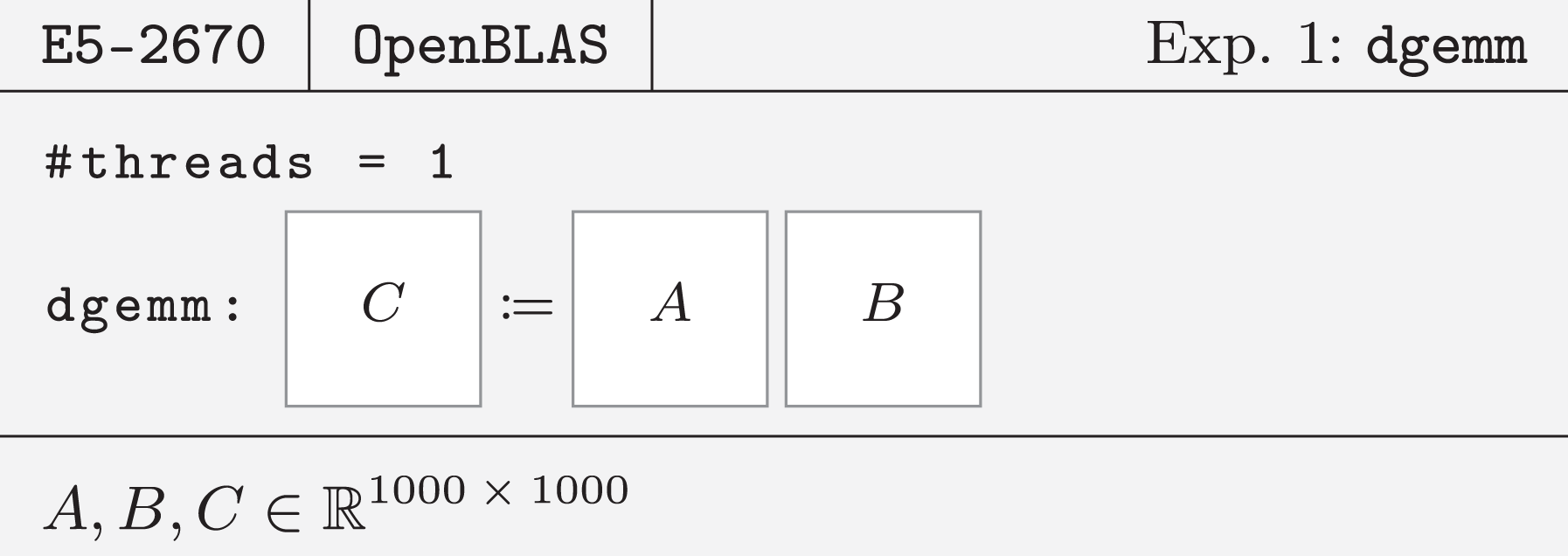
As shown schematically above, this experiment runs on one core of an Intel Sandybridge E5-2670 processor, using the OpenBLAS library (Xianyi), and executes the double precision kernel dgemm once on random square matrices of size 1000 × 1000. Although simple, similar experiments are commonly used to determine the attainable peak performance of a given processor.

When combined with additional information on the hardware and the kernel’s complexity, the raw timing (in cycles) from this experiment leads to a number of metrics, which yield more insights into how efficiently the CPU is used.

Metric	Value
Cycles	272,551,028
Time (ms)	104.8
Gflops/s	19.1
flops/cycle	7.3
efficiency (%)	91.7

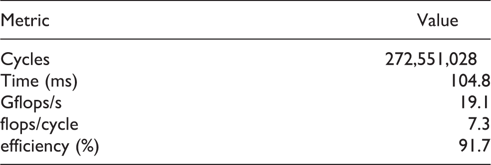
Furthermore, if available, the PAPI (Browne et al., 2000) provides access to useful hardware counters.

Metric	Counter name	Value
Level 1 cache misses	PAPI_L1_TCM	32,933,961
Conditional branches mispredicted	PAPI_BR_MSP	3941

With ELAPS, all these metrics are readily available and easily extensible.

3.1. Repetitions and statistics

Multiple executions of a kernel often result in fluctuating timings; the reasons for such differences include library initialization overhead, cache locality, and system jitter. As customarily done, in ELAPS, this issue is addressed by repeating each experiment several times while collecting statistics. As an example, let us consider an experiment that repeats the kernel execution 10 times on the same input matrices (i.e. the same memory locations):

This second experiment produces 10 measurements, from which we derive statistics as those presented in Figure 1: We chose to visualize all data points (all), the mean and a band of one standard deviation (std), a box plot (box), and a violin plot (violin). It is worth pointing out that whenever multiple repetitions are executed and timed, the first one almost inevitably represents an outlier; for the most part, this phenomenon is connected to the initialization of the kernel library, but it is also due to the loading and caching of data and instructions. In general, a more accurate representation of the effective performance is obtained by dropping the first measurement of the lot. In Figure 1, one can appreciate how significantly the first repetition affects various statistics, and most noticeably the minimum (exposed in the violin plot), mean, and standard deviation.

Figure 1.

Performance statistics from 10 repetitions of dgemm.

In order to avoid the impact of “first-execution” outliers, in all following examples and studies, we always discard the measurement from the first repetition.

3.2. Data placement: Varying operands

In experiment 2, the matrices A, B, and C were reused across repetitions, causing them to stay in cache; this scenario is also known as “warm data.” Depending on the application, the assumption of warm data may or may not be realistic; to reflect this in our experiments, we allow to “vary” the operands (i.e. use different memory locations) individually in each repetition. Furthermore, in ELAPS, one can freely control the relative position of varying operands: They can be stacked horizontally or vertically (indicated by a subscript ↓), with or without an arbitrary offset.

In the following experiment, while A and B are fixed and quite small, C varies in each repetition (hence the subscript in C _rep) and is therefore never cached (“cold data”).

In Figure 2, we present the results of experiment 3 and another experiment in which the matrices A, B, and C are all fixed. The performance loss due to the enforced out-of-cache scenario for C is clearly visible.

Figure 2.

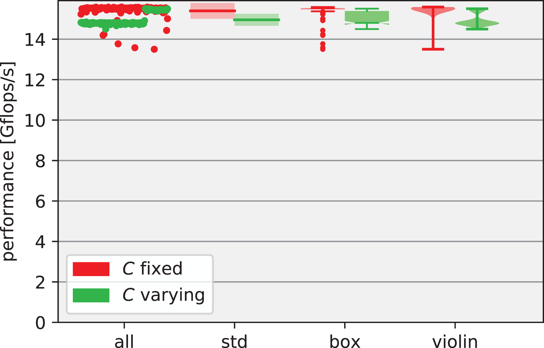
Influence of data locality on dgemm.

3.3. Sequences of kernels

In addition to isolated kernels, allows to experiment with sequences of calls. Let us use the solution of a linear system as an example: The problem

is typically solved by first LU-decomposing A (dgetrf), and then solving two triangular linear systems (dtrsm). The process—which is also implemented in LAPACK’s dgesv—is replicated in experiment 4.¹

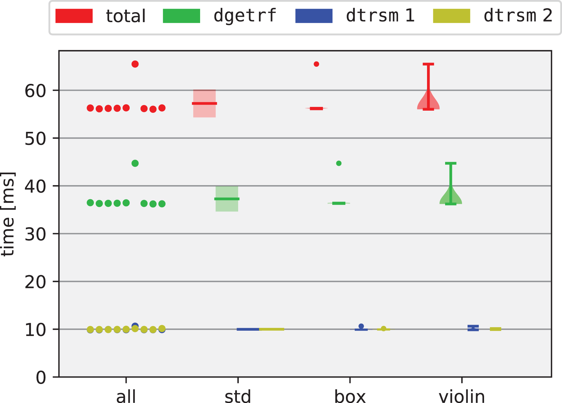
For this experiment, Figure 3 shows both the total execution time and the time spent in each individual kernel. It is easy to see that for 200 right-hand sides, the LU decomposition dgetrf is responsible for more than 60% of the total execution time, while each of the dtrsm’s only contribute less than 20%.

Figure 3.

Breakdown of the timings for the solution of a linear system.

3.4. Parameter range

So far, we only considered experiments in which the sizes of the kernel operands were fixed. In many practical experiments, however, one wants to study the performance of a routine over a range of parameters. In the following example, we use the routine dgesv, which solves a linear system directly, to solve problems of size n with 500 right-hand sides, where n ranges from 50 to 2000 in steps of 50.

Performance results from experiment 5 are shown in Figure 4; the plot displays the increase in performance for increasing problem size, as typical for dense linear algebra kernels.

Figure 4.

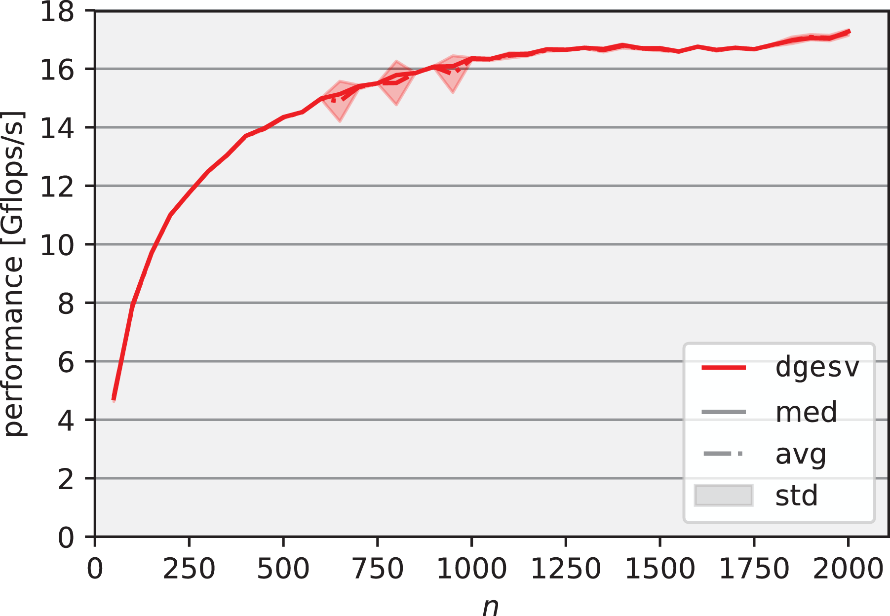
Solution of linear systems: performance.

3.5. Threads range

Scalability studies are extremely common examples of experiments that make use of ranges. In the following experiments, we compute the eigenvalue decomposition of a symmetric matrix (of fixed size) using 1 up to 8 threads, and compare LAPACK’s solvers dsyev, dsyevx, dsyevr, and dsyevd (see Anderson et al. (1999) for details on these routines).

As one can appreciate from Figure 5, ELAPS makes it easy to set up, execute, and compare the results of multiple experiments with varying degrees of parallelism.

Figure 5.

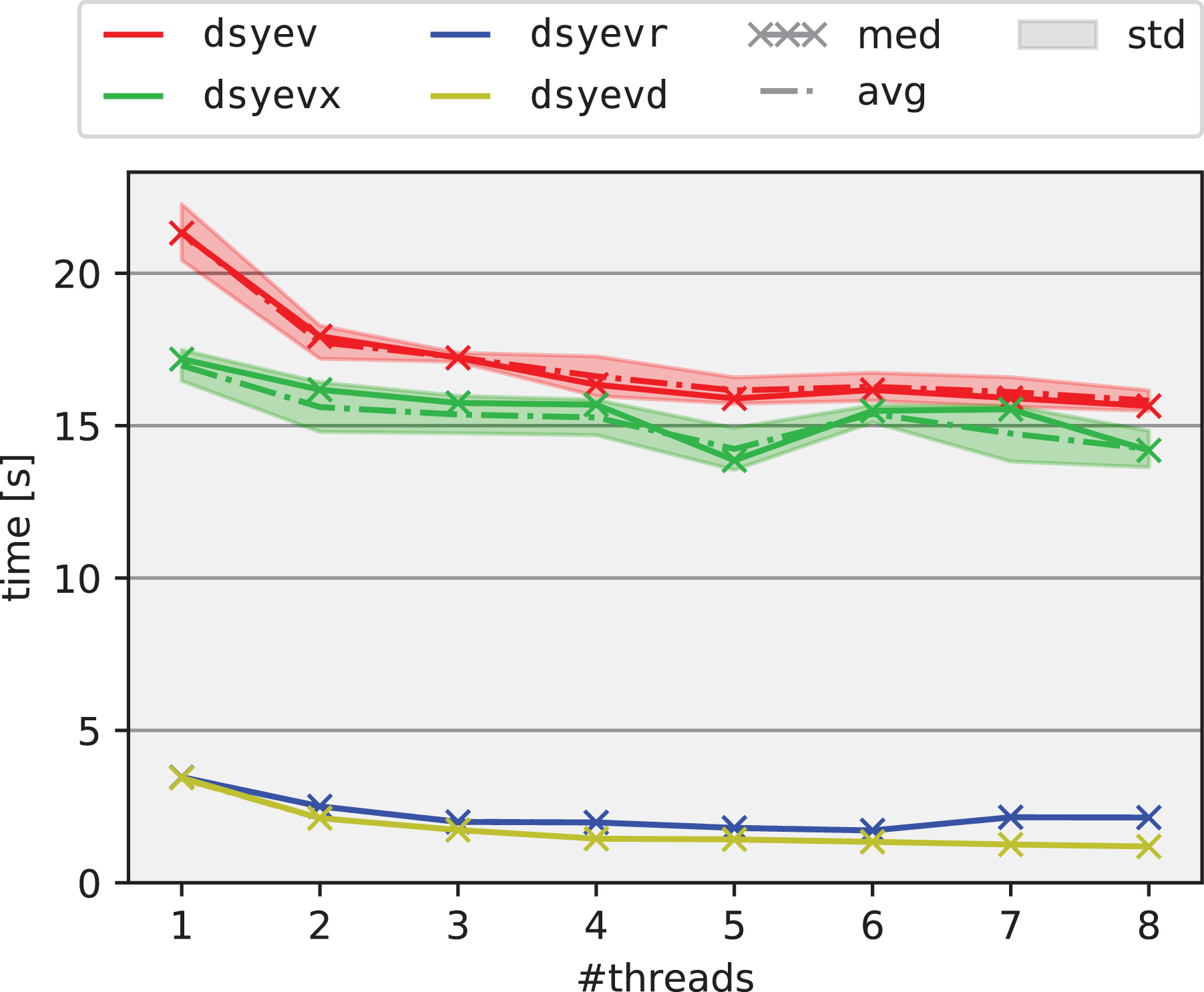
Scalability of LAPACK’s symmetric dense eigensolvers on random matrices.

3.6. Sum- and OpenMP-range

In loop-based algorithms, the total execution time is often more meaningful than an iteration-by-iteration breakdown. For this purpose, in addition to the “parameter range” described in the previous subsection, ELAPS also provides a “sum-range,” which yields the total contribution of the loop. For instance, experiment 7 models the inversion of a lower triangular matrix² of size 1000 via a blocked algorithm that traverses the matrix in steps of a fixed block size b.

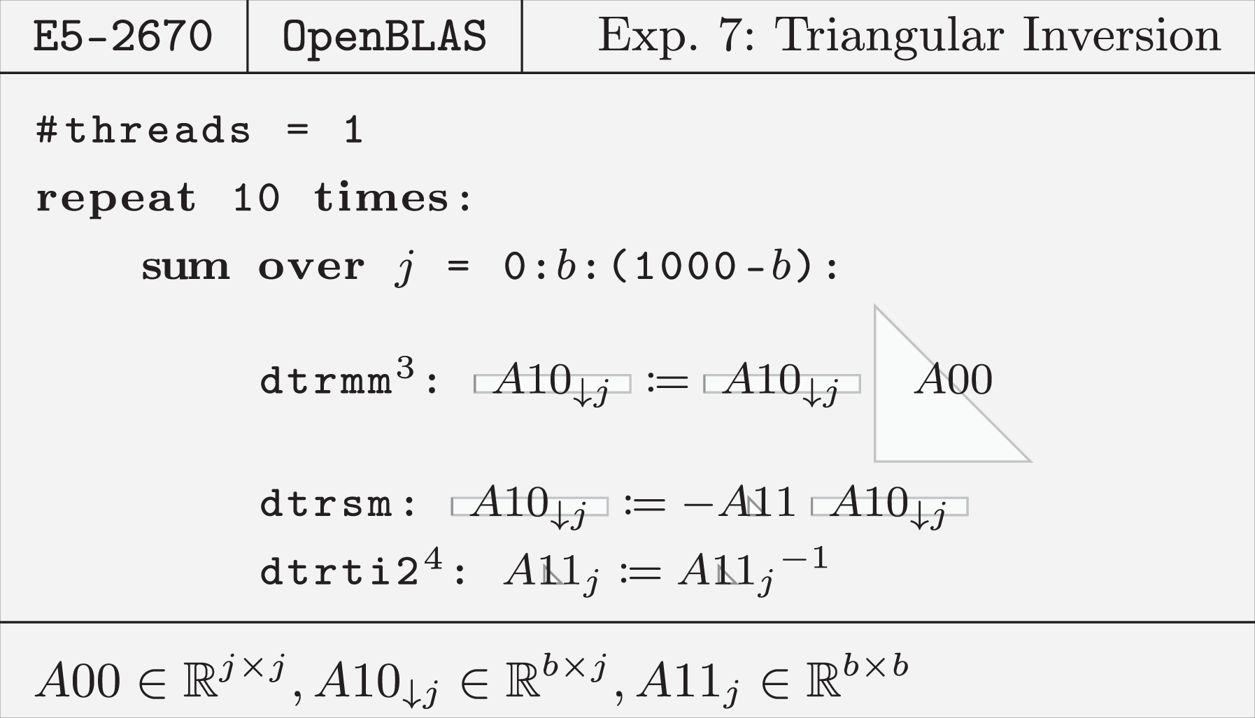
Figure 6 reports the performance attained by this algorithm for different block sizes b; the maximum is observed for b = 100. The choice of parameters represents an important step to tailor algorithms for a given architecture; for instance, the tuning of block sizes is required by many of the algorithms included in LAPACK (Anderson et al., 1999; Whaley, 2008). Notice that a simpler and finer-grained experiment to optimize the block size is obtained by combining the sum range with a parameter range for b.

Figure 6.

Influence of block size on triangular inversion.

OpenMP-range multi-threading can typically be exploited in two different ways, namely, either invoking a multi-threaded library (such as OpenBLAS) or through OpenMP. To investigate these alternatives, in experiments 8 and 9, we implement the solution of a triangular linear system with a tall and skinny right-hand side (1) with OpenBLAS’s threaded dtrsm kernel and (2) as a series of parallel dtrsv’s⁵ using ELAPS’s OpenMP-range.

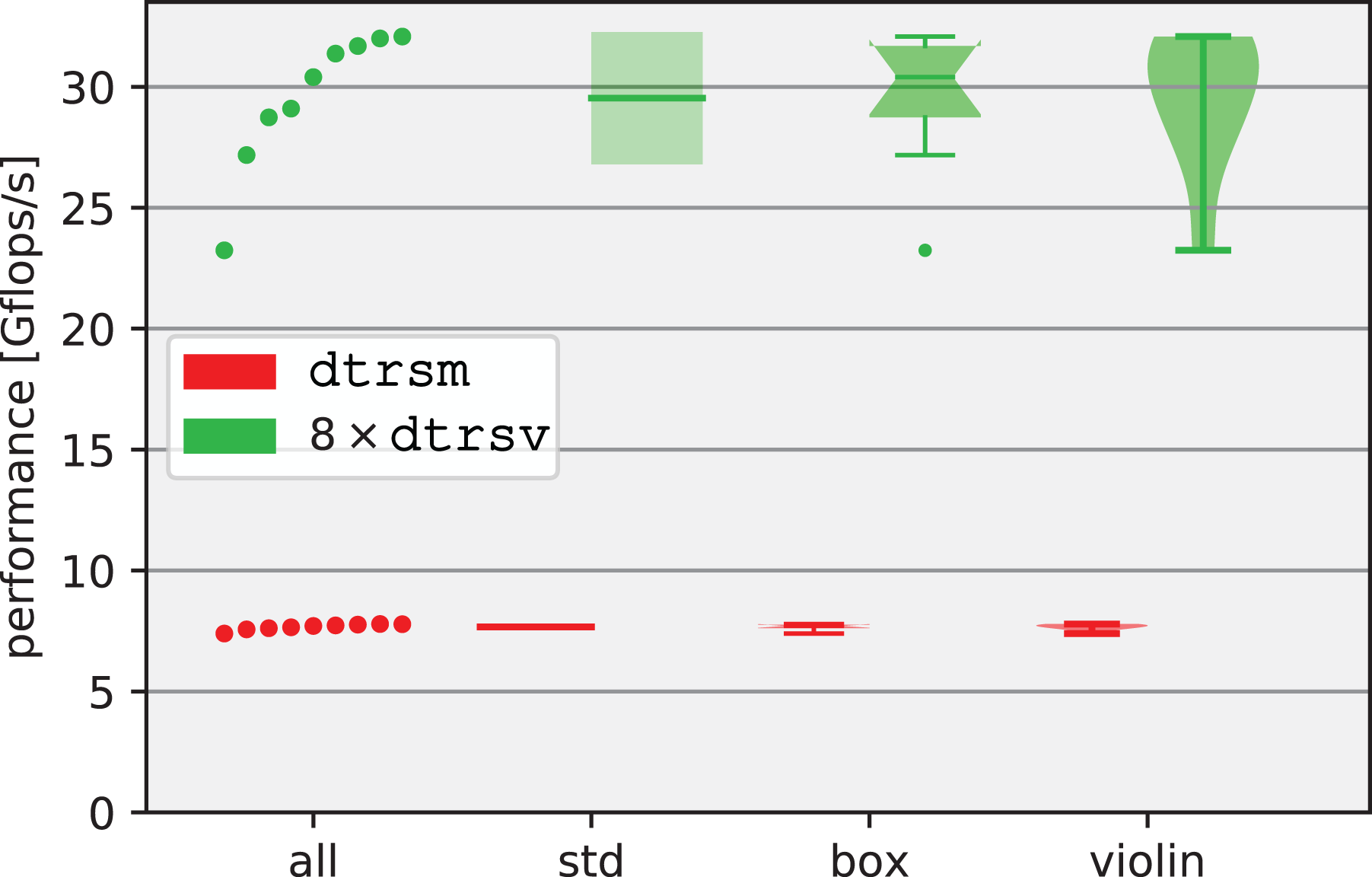
The results in Figure 7 suggest that the parallel dtrsv’s are considerably faster than the threaded dtrsm’s, indicating that OpenBLAS is not optimally parallelized for such extremely skewed matrix sizes.

Figure 7.

Performance of threaded dtrsm versus parallel dtrsv.

4. The ELAPS framework

The ELAPS framework is built to support performance experiments combining the features and scenarios described in Section 3. In this section, we present the structure of the framework, focusing on the aspects that make it general and intuitive, yet powerful. A more user-oriented guide can be found as part of its documentation on GitHub: http://github.com/HPAC/ELAPS.

As shown in Figure 8, ELAPS is structured in three layers.

The first, “bottom” layer is written in C/C++ and contains the Sampler, a low-level command line tool responsible for executing and timing individual kernels. The Sampler has to be compiled for each specific combination of hardware and libraries (the only stage in which the user needs to configure the system); ELAPS can interface with any number of Samplers.

The second, “middle” layer is the Python library elaps, which centers around the class Experiment that implements the previously introduced experiments. An Experiment can be executed on different Samplers, both locally or through batch-job systems. The outcome is a Report, which provides not only structured access to the individual measurements, but also functionality to analyze different metrics and statistics.

This layer also includes the plot module, which is based on the matplotlib library, and is used to easily visualize Reports in graphical form.⁶

The third, “top” layer adds a graphical user interface, written in PyQt4, to both design Experiments in the PlayMat and study Reports and plots in the Viewer.

Figure 8.

Structure of the ELAPS framework.

The design of these three layers is discussed in the next subsections.

4.1. The Sampler

The Sampler is a low-level performance measurement tool tailored to dense linear algebra operations at the core of the ELAPS framework. This tool, earlier versions of which were already utilized by Peise and Bientinesi (2012) and Peise et al. (2015), makes it possible to measure the performance of individual kernel executions, implementing the following workflow:

read from standard input a list of calls, that is, kernel names with corresponding lists of arguments;

execute the specified calls, thereby measuring their performance in terms of CPU cycles, and optionally through performance counters provided by the PAPI;

print the measured performance numbers to the standard output.

While reading the list of kernels from the standard input, the Sampler accepts several special commands: go executes, measures, and reports the results of all previously read calls; {omp and }, respectively, start and end a list of calls to be executed as parallel OpenMP tasks; set_counters sets the PAPI counters for the next set of executions.

The Sampler accepts kernels and arguments in a format that agrees with the conventions used by standard libraries such as Basic Linear Algebra Subroutines (BLAS) and LAPACK: Each argument is passed by reference, and is of type char *, int *, float *, or double *.

In a dense linear algebra kernel, these arguments are of one of two types.

Scalar arguments point to scalar values, some of which may influence the kernel’s behavior and control flow. Examples include: flag arguments (e.g. side, transA), size arguments (e.g. m, n), scalars (e.g. alpha, beta), and leading dimensions (e.g. ldA, ldB).

Within the Sampler, scalar argument values are stored consecutively in an array.

Data arguments point to memory regions that hold the mathematical objects (such as vectors or matrices) involved in the kernel call. Generally,⁷ the actual contents of these arguments do not affect the control flow; nonetheless, these arguments may still have a significant impact on performance, depending on their location in the memory hierarchy.

The Sampler has two mechanisms to treat data arguments:

Named variables are designated memory regions referenced by a variable names. A set of features to allocate ( xmalloc ⁸), compute offsets into ( xoffset) and free (free) such variables give users full control over where operands are stored in relation to each other.

Dynamic memory offers a fast way to pass “unnamed” memory regions as data arguments. Within one call, all such regions are guaranteed to be disjoint; across calls, however, the same memory regions may be reused arbitrarily.

To set up the contents of data arguments, the Sampler provides a set of simple utility-type kernels: xmemset fills every entry in a buffer with a single value, xgerand fills it with random values (uniform in ]0, 1[), and xporand generates a random symmetric (or Hermitian) positive definite matrix. Furthermore, xreadfile and xwritefile, respectively, read matrices from and write them to binary files.

4.2. The elaps package

The middle layer of the ELAPS framework centers around the experimental features introduced in Section 3, encoded in the Python class Experiment. Instances of this class form the starting point for performance experiments; executing them using Samplers ultimately leads to Reports, which can be analyzed with respect to a variety of metrics and statistics.

4.2.1. Experiments

Experiment instances are both a static description of experiments, which are easily stored to and loaded from strings and files for portability, but also feature functionality to support their design and handling.

The kernel configurations at the center of each experiment are its connection to libraries such as BLAS or LAPACK. While the interfaces of such libraries aim to be general by accommodating multiple functionalities, precisely because of their generality they are often unintuitive and hard to memorize. To counter this problem, elaps uses optional “Signatures” to annotate kernels, thereby providing possible value ranges and semantic connections between arguments. In the end, these Signatures allow Experiments to expose feasible values for arguments (such as trans or uplo) and automatically derive connected arguments such as operand sizes and leading dimensions, both within a single kernel and across multiple kernels. As an example, Figure 9 shows ELAPS’s built-in Signature for dtrsm.

Figure 9.

ELAPS Signature for dtrsm.

The execution of an Experiment is initiated by the submit method, which first generates the sequence of kernel calls for the Sampler and a shell script for its execution, and then either executes this script locally or submits it to a batch-job system.

4.2.2. Execution on Samplers

In this section, we describe how the Experiment features are translated into commands for the Sampler.

As input, the Sampler expects a raw list of kernel invocations. To produce this list, all ranges and repetitions in an Experiment are completely unrolled, thereby evaluating any symbolic (range-dependent) variables. The OpenMP-range is translated directly to the Sampler’s {omp and} commands. Using the parameter range to vary the number of library threads requires to interface with said library; to avoid library-dependent kernels and Sampler features, we do so through environment variables (e.g. OPENBLAS_ NUM_THREADS) and by starting the sampler separately for each thread count.

Data arguments in kernels are allocated as named variables in the Sampler at the beginning of the input. Arguments that vary with repetitions or the sum/OpenMP-range (i.e. they point to different locations) are first allocated as a single large block and then subdivided by calculating appropriate offsets, resulting in individual variables for each repetition and range iteration.

Finally, PAPI counters are also set at the beginning through the set_counters command.

4.2.3. Reports

Each Experiment execution results in a report file that, when read into elaps, turns into a Report instance. This object serves as a structured representation of the obtained measurements with respect to the underlying Experiment: Raw measurements are accessed through the hierarchy “parameter-range value → repetition → sum/OpenMP-range value → kernel” and yield the cycle count or PAPI counter measurements. Separately, a “reduced” view on the results accumulates the sum/OpenMP-range and the kernels according to the experiment semantic.

To turn these structured yet raw measurement results into more meaningful quantities, metrics combine them with the kernels’ Floating Point Operation (FLOP) counts and information on the execution environment. The easily extensible set of metrics ranges from “execution time in seconds” to “Gflops/s” and “efficiency.”

While a metric converts measurements values one-by-one, results from multiple repetitions are combined by statistics, such as “minimum,” “maximum,” “median,” or “standard deviation.” As motivated in Section 3, the results from the first repetitions are optionally discarded to hide overhead effects and make statistics more representative of in-application invocations.

4.2.4. Plotting

ELAPS’s plot module generates matplotlib figures from the structured data in Reports under consideration of both metrics and statistics. Depending on the type of experiment, it automatically generates appropriate bar or line plots that are easily exported to various file formats.

4.3. The graphical user interface

ELAPS’s Experiment and Report Python classes establish a flexible and powerful foundation for performance evaluations at a scripting level. In order to enable performance experimentation in an explorative fashion and to facility more intuitive interaction, ELAPS features a graphical user interface. As shown in Figure 8, this interface consists of two components: While the PlayMat serves as a “playing mat” to develop Experiments, the Viewer interactively visualizes Reports.

The PlayMat, shown in Figure 10(a), allows interactive access to the full functionality of an Experiment. To further guide the user, among other things, it visualizes the Experiment’s kernels based on their Signatures (similar to how they are presented in this article) and automatically calculates matrix sizes and (if desired) deducible arguments, such as leading dimensions. It furthermore offers kernel documentations as tootips, provides progress tracking of executing Experiments and can load completed Reports directly in the Viewer.

Figure 10.

ELAPS’s graphical user interface. ELAPS: Experimental Linear Algebra Performance Studies.

The Viewer, shown in Figure 10(b), is an interactive means to analyze and compare Reports. It provides all metrics applicable to the selected Reports, and its statistical plots are easily manipulated and exported.

5. Application examples

In this section, we demonstrate the use of the ELAPS framework in several application examples. For this purpose, we deliberately chose a wide range of hardware systems and kernel libraries.

5.1. Algorithm selection: Tensor contractions

Let us consider the tensor contraction (in Einstein notation)

C_{a b c} := A_{a k} B_{k c b}

with $A \in ℝ^{1250 \times 750}$ , $B \in ℝ^{750 \times 500 \times n}$ , and $C \in ℝ^{1250 \times n \times 500}$ , where n is between 100 and 1000. Using an explicit index notation, C is computed as

\forall a, \forall b, \forall c . C [a, b, c] := \sum_{k} A [a, k] \cdot B [k, c, b]

and can be visualized as follows:

A natural approach to efficiently compute such tensor contractions is to utilize the highly optimized dgemm kernel. For contraction (2), there are two ways of casting the computation as a series of dgemm’s:

An inspection of these algorithms reveals that they both execute a dgemm of fixed size on varying data; in particular, the number of invocations in algorithms “∀b” and “∀c” (respectively, (4) and (5)) are, respectively, n and 500. By virtue of this observation, experiments 10 and 11 only perform 10 repetitions, thus reducing the experimentation time; while the results will not be meaningful estimates for the total execution time, they will expose the same computational efficiency (expressed in Gflops/s) as the full algorithms. Furthermore, since algorithm “∀b” operates on matrices of fixed size and independent of n, in experiment 10, we also avoid the use of the parameter range.

We perform experiments 10 and 11 on a 16-core IBM PowerPC A2 node of the IBM BlueGene installation JUQUEEN at the Jülich Supercomputing Center, Jülich, Germany linked to IBM’s optimized ESSL library. Only the Sampler is executed on this compute node, running the lightweight CNK operating system; it is accessed by elaps from a Red Hat Enterprise Linux 6.6 front-end node through the LoadLeveler batch-job system.

Figure 11 suggests that neither of the two algorithms is optimal for all cases: While for a small dimension n, algorithm “∀b” is better, algorithm “∀c” dominates for large n. Interestingly, the crossover point is not at n = 500, where both algorithms work with matrices of equal size, but already around n = 300.

Figure 11.

Comparison of dgemm-based algorithms for tensor contraction (2).

5.2. Library selection: Sylvester equation

Choosing the right library can be a crucial step in attaining high performance. In this section, we demonstrate its importance by considering the triangular Sylvester equation

to be solved for X, which is central to problems in control theory. In addition to LAPACK’s dtrsyl, several other libraries offer a kernel with the same interface. In our tests, we consider

LAPACK 3.5 (Anderson et al., 1999) linked to OpenBLAS 0.2.14 (Xianyi);

RECSY 0.01 (Jonsson and Kågström, 2003) linked to OpenBLAS;

libFLAME ⁹ 5.1.0-18 (Quintana-Ortí and van de Geijn, 2003; Zee, 2009) linked to OpenBLAS; and

Intel’s commercial Math Kernel Library (MKL) 11.0 (Intel a).

To compare these libraries, we launch experiment 12 on a 10-core Intel IvyBridge E5-2680 v2 processor with Samplers linked to the above-mentioned libraries. This machine, which is part of a compute cluster, is accessed through the Platform LSF 9.1.2 batch-job system with both the front-end (elaps) and back-end (the Samplers) running Scientific Linux 6.6.

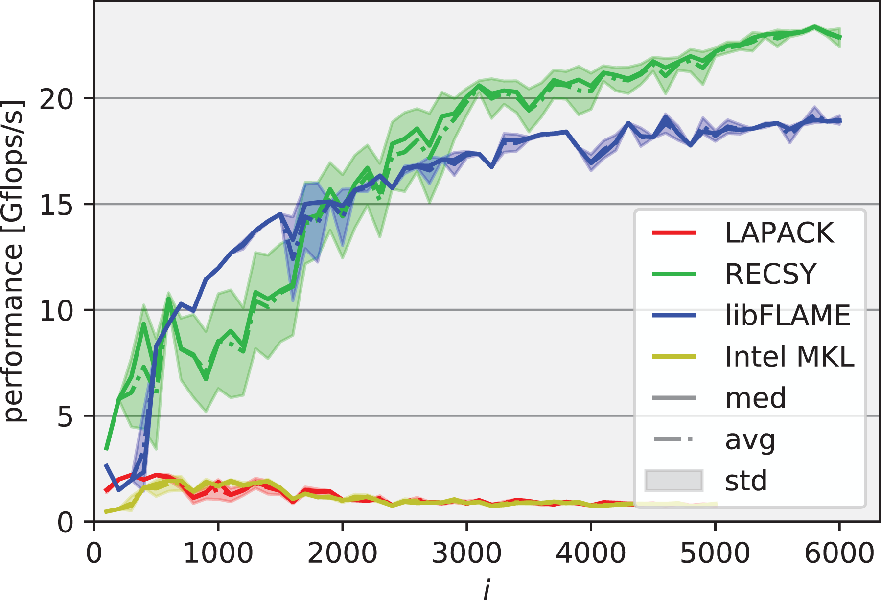
Figure 12 shows the performance attained by the different libraries. LAPACK, which only provides an unblocked algorithm for dtrsyl, reaches 2 Gflops/s for small problems but eventually falls below 1 Gflops/s. The specialized RECSY library on the other hand attains the best performance of up to 22.9 Gflops/s. libFLAME is initially competitive with RECSY but eventually plateaus at 18.9 Gflops/s. Surprisingly, the otherwise very efficient MKL seems poorly optimized for this problem and is as fast as LAPACK.

Figure 12.

Comparison of libraries for the triangular Sylvester equation.

5.3. Multi-threading: Sequence of LUs

In a certain type of electronic structure calculations (Bauer and Blügel, 2013), one has to solve a series of fairly small linear systems. As already mentioned, a possible approach involves the LU decomposition (dgetrf) and two triangular linear systems (dtrsm) for each matrix; since each system only involves two right-hand sides, the cost for the dtrsm’s is entirely negligible.

On multi-core machines, the sequence of LUs can be parallelized at the granularity of one matrix via a multi-threaded dgetrf kernel, or by assigning different matrices to different threads via OpenMP (hybrid solutions are also possible). Performance-wise, there are arguments both in favor and against each of these two alternatives: Using BLAS’s internal parallelism ensures that only one kernel uses the CPU’s caches at a time; on the other hand, OpenMP’s parallelism increases the amount of work that the CPU’s cores can perform simultaneously.

The next three experiments use ELAPS’s sum range and OpenMP range constructs to model the scenarios in which (1) a multi-threaded kernel is used, (2) OpenMP runs sequential kernels in parallel, and (3) OpenMP runs multi-threaded kernels in parallel.¹⁰ Each of them measures the time it takes to LU-decompose an increasing number of square matrices of size 800.

These three experiments are executed on a MacBook Pro running OS X 10.9.4 with a quad-core Intel Haswell i7-4850HQ CPU (Turbo Boost disabled) using Apple’s Accelerate framework; both the Sampler and elaps run on the same platform.

Figure 13 indicates that of the two “pure” approaches, when more than eight LUs are performed (i.e. more than the CPU has hardware threads), OpenMP with single-threaded kernels outperforms Accelerate’s parallel kernel. However, the mixed approach, in which Accelerate uses up to eight threads, while OpenMP is allowed to schedule the LU decomposition tasks, is even more efficient, reaching up to 75 Gflops/s.

Figure 13.

Multithreading paradigms for a sequence of LUs.¹³

5.4. Algorithmic optimization: Genome wide association studies

Genome wide association studies (GWAS) investigate how human traits (e.g. eye color or genetic diseases) are related to certain locations in the human genome (Boerwinkle et al., 1986; Yu et al., 2006). Computationally, GWAS can be cast as a sequence of generalized least squares (GLS) problems

where $M \in ℝ^{n \times n}$ is symmetric positive definite, $X_{i} \in ℝ^{n \times p}$ , $y \in ℝ^{n}$ , and $b_{i} \in ℝ^{p}$ with 1000 ≤ n ≤ 5000, p ≤ 20 and $i \in {1, \dots, m}$ , where m can be in the millions.

A straightforward implementation of this equation (e.g. using R or MATLAB) might compute each b_i individually by solving equation (7) from right to left, as modeled in this next experiment (with n = 1000 and p = 4):

For experiment 15, we choose a 60-core Intel Xeon Phi coprocessor using Intel MKL. ELAPS’s python library and the PlayMat are run on this system’s Host processor (Scientific Linux 6.6); only the Sampler is executed natively on the coprocessor.

Figure 14 shows both the execution time of experiment 15, as well as a breakdown thereof. The runtime is clearly dominated by the dposv and dtrsm kernels involving M.

Figure 14.

Timing breakdown for a sequence of GLS solves. GLS: generalized least squares.

From a first analysis of these two kernels, one realizes that the dposv ( $y : = M^{- 1} y$ ) is independent of the loop index i, thus it can be taken out of the loop and computed just once. This modification reduces dposv’s contribution to the total runtime by a factor of m, effectively shifting the bottleneck onto dtrsm.

A further analysis reveals that all the dtrsm linear systems involve the same matrix M; this observation suggests to combine the right-hand sides $X_{i} \in ℝ^{m \times 4}$ for all m iterations into a single large matrix $X \in ℝ^{1000 \times 4 m}$ . The following experiment solves a linear system with this matrix as the right-hand side with a single invocation of dtrsm:

For the selected range of m, the runtime of this experiment is around 115 ms, i.e., already more than one order of magnitude less than the previous experiment. Furthermore, for larger problems, the dtrsm kernel can make good use of the coprocessor’s many cores and reaches over 550 Gflops/s. For an in-depth study of performance optimizations for GWAS, we refer the reader to (Fabregat-Traver et al., 2014) and (Fabregat-Traver and Bientinesi, 2014).

6. Productivity study

Ultimately, ELAPS’s main purpose is to increase the productivity of application developers by providing a simple, yet powerful, performance experimentation framework for dense linear algebra operations. In order to evaluate the productivity gain (over traditional, handwritten performance experiments) achieved when using ELAPS, we conducted a productivity study. Specifically, we chose 10 individuals with considerably different backgrounds in linear algebra and high-performance computing, ranging from novice (approaching BLAS and LAPACK for the first time), to expert (developer of linear algebra libraries), yet all without prior experience with ELAPS.

The test subjects were asked to repeat the same performance study twice—first with ELAPS, then using C and any visualization tool (gnuplot, Python, MATLAB, etc.)—and to report both the time investment and the overall development experience. The specific task was to replicate the tensor contraction performance study detailed in Section 5, generate a figure similar to Figure 11, illustrate the fluctuations in the measurements, and identify the crossover (if any) between the two algorithmic alternatives. The subjects chose their own hardware and software setup.

Across the board, the subjects reported a productivity boost. Despite the fact that the study was first performed with ELAPS—including the solution-independent problem analysis and understanding—in all cases it was reported that with ELAPS the process was faster. The speedups ranged between 4× and 9×, and the average productivity boost was of a factor of 6. In particular, the experiment setup, execution, and evaluation in ELAPS took on average around 10–12 min (including familiarization with the user interface), while the handwritten benchmarks and their evaluation took most subjects more than 1 h.

The participants stressed that the increase in productivity was not only due to the simple experiment setup in the PlayMat, but also to the Viewer as an intuitive and powerful post-processing and visualization tool. They furthermore pointed out the ease with which experiments are modified to inspect different performance aspects. Finally, the participants felt that their own individual setups were far more prone to errors and required extensive testing, while ELAPS allowed them to ignore such “mundane task.”

7. Conclusion

We introduced the ELAPS framework, a set of tools and features to easily experiment and interact with dense linear algebra operations. Similar to how high-level frameworks such as MATLAB and Mathematica enable fast prototyping of new ideas, ELAPS enables the fast investigation of performance-related aspects of linear algebra algorithms; this is achieved by allowing users to easily design, execute, measure, and analyze algorithms. In contrast to the traditional “features first, performance later” approach, this investigation takes place before any actual coding, and serves to gain insights towards high-performance implementations.

Throughout this article, we applied ELAPS to a wide range of scenarios, including parameter optimization (Section 3), algorithm selection (Sections 3 and 5), library comparison (Section 5), and parallelism and library threading (Sections 3 and 5). We demonstrated the framework’s flexibility by linking it with seven kernel libraries, and by executing experiments on five different platforms, including a Xeon Phi coprocessor and two batch-job systems. In summary, ELAPS covers many aspects of shared-memory optimizations, a critical step towards achieving large-scale performance.

Having established the foundations of a framework for rapid experimentation, we foresee many opportunities for extensions. In particular, we envision (1) coverage of a broader range of architectures, including GPUs and ARM-based CPUs, (2) support for metrics related to data movement and energy consumption, and (3) interfaces for kernels and paradigms of distributed-memory libraries such as ScaLAPACK (Blackford et al., 1997) and Elemental (Poulson et al., 2013).

Footnotes

Software

ELAPS is open source (BSD license) and available on GitHub:

Acknowledgements

The authors would like to thank their colleagues in the HPAC research group for many fruitful discussions and valuable feedback, and the Jülich Supercomputing Centre (JSC) for providing access to JUQUEEN.

Declaration of Conflicting Interests

The author(s) declared no potential conflicts of interest with respect to the research, authorship, and/or publication of this article.

Funding

The author(s) disclosed receipt of the following financial support for the research, authorship, and/or publication of this article: This work was supported by the Deutsche Forschungsgemeinschaft (DFG) through grant GSC 111 and the Deutsche Telekom Stiftung.

Notes

References

Anderson

Bai

Bischof

. (1999) LAPACK Users’ Guide, 3rd ed. Philadelphia, PA: Society for Industrial and Applied Mathematics. ISBN 0-89871-447-8 (paperback).

Bauer

DSG

Blügel

(2013) Development of a relativistic full-potential first-principles multiple scattering Green function method applied to complex magnetic textures of nano structures at surfaces. PhD Thesis, Jülich. Available at: http://publications.rwth-aachen.de/record/229375. Druck-Ausgabe: 2013. - Online-Ausgabe: 2014; Zugl.: Aachen, Techn. Hochsch., Diss., 2013. (accessed 8 March 2018).

Bientinesi

Igual

Kressner

. (2011) Condensed forms for the symmetric eigenvalue problem on multi-threaded architectures. Concurrency and Computation: Practice and Experience 23(7): 694–707.

Blackford

Choi

Cleary

. (1997) ScaLAPACK Users’ Guide. Philadelphia, PA: Society for Industrial and Applied Mathematics. ISBN 0-89871397-8 (paperback).

Boerwinkle

Chakraborty

Sing

(1986) The use of measured genotype information in the analysis of quantitative phenotypes in man. I. Models and analytical methods. Annals of Human Genetics 50(Pt 2): 181–194.

Browne

Dongarra

Garner

. (2000) A portable programming interface for performance evaluation on modern processors. International Journal of High Performance Computing Applications 14(3): 189–204. DOI: 10.1177/ 109434200001400303.

Chen

Hollingsworth

(2013) Towards fully automatic auto-tuning: leveraging language features of chapel. International Journal of High Performance Computing Applications 27(4): 394–202. DOI: 10.1177/1094342013493198.

Demmel

Marques

Parlett

. (2008) Performance and accuracy of LAPACK’s symmetric tridiagonal eigensolvers. SIAM Journal on Scientific Computing 30(3): 1508–1526. DOI: 10.1137/070688778.

Fabregat-Traver

Bientinesi

(2014) Computing petaflops over terabytes of data: the case of genome-wide association studies. ACM Transactions on Mathematical Software (TOMS) 40(4): Article 27:1–27:22.

10.

Fabregat-Traver

Aulchenko

Bientinesi

(2014) Solving sequences of generalized least-squares problems on multi-threaded architectures. Applied Mathematics and Computation 234: 606–617.

11.

Frigo

Johnson

(2005) The design and implementation of FFTW3. Proceedings of the IEEE 93(2): 216–231. Special issue on “Program Generation, Optimization, and Platform Adaptation.”

12.

Geimer

Wolf

Wylie

BJN

. (2010) The Scalasca performance toolset architecture. Concurrency and Computation: Practice and Experience 22(6): 702–719. DOI: 10.1002/cpe.v22:6.

13.

Hurault

Baek

Casanova

(2014) Selecting linear algebra kernel composition using response time prediction. Software: Practice and Experience 45(12): 1659–1676. DOI: 10.1002/spe.2307.

14.

Intel (a) Math Kernel Library (MKL). Available at: https://software.intel.com/en-us/intel-mkl (accessed 8 March 2018).

15.

Intel (b) VTune Amplifier. Available at: https://software.intel.com/en-us/intel-vtune-amplifier-xe (accessed 8 March 2018).

16.

Jonsson

Kågström

(2003) RECSY – a high performance library for Sylvester-type matrix equations. In: Kosch

Böszörményi

Hellwagner

(eds), Euro-Par 2003 Parallel Processing, Lecture Notes in Computer Science, vol. 2790. Springer Berlin Heidelberg, pp. 810–819. DOI: 10.1007/978-3-540-45209-6_111.

17.

Nagel

Arnold

Weber

. (1996) VAMPIR: visualization and analysis of MPI resources. Supercomputer 12: 69–80.

18.

Peise

Bientinesi

(2012) Performance modeling for dense linear algebra. In: Proceedings of the 2012 SC Companion: High Performance Computing, Networking Storage and Analysis (PMBS12), SCC ‘12. Washington, DC, USA: IEEE Computer Society, pp. 406–416.

19.

Peise

Fabregat-Traver

Bientinesi

(2015) On the performance prediction of BLAS-based tensor contractions. In: Jarvis

Wright

Hammond

(eds), High Performance Computing Systems. Performance Modeling, Benchmarking, and Simulation, Lecture Notes in Computer Science, vol. 8966. Cham, Switzerland: Springer International Publishing, pp. 193–212.

20.

Poulson

Marker

van de Geijn

. (2013) Elemental: a new framework for distributed memory dense matrix computations. ACM Transactions on Mathematical Software 39(2): 13:1–13:24. DOI: 10.1145/2427023.2427030.

21.

Quintana-Ortí

van de Geijn

(2003) Formal derivation of algorithms: the triangular Sylvester equation. ACM Transactions on Mathematical Software 29(2): 218–243. DOI: 10.1145/779359.779365.

22.

Schaefer

Pankratius

Tichy

(2009) Atune-IL: an instrumentation language for auto-tuning parallel applications. In: Sips

Epema

Lin

(eds), Euro-Par 2009 Parallel Processing, Lecture Notes in Computer Science, vol. 5704. Springer Berlin Heidelberg, pp. 9–20. DOI: 10.1007/978-3-642-03869-3_5.

23.

Shende

Malony

(2006) The Tau parallel performance system. International Journal of High Performance Computing Applications 20(2): 287–311. DOI: 10.1177/1094342006064482.

24.

Ţăpuş

Chung

Hollingsworth

(2002) Active harmony: towards automated performance tuning. In: Proceedings of the 2002 ACM/IEEE conference on supercomputing, SC ‘02, Baltimore, Maryland, 16–20 November 2002, pp. 1–11. Los Alamitos, CA, USA: IEEE Computer Society Press. Available at: http://dl.acm.org/citation.cfm?id=762761.762771 (accessed 8 March 2018).

25.

Whaley

(2008) Empirically tuning LAPACK’s blocking factor for increased performance. In: Computer science and information technology, 2008. IMCSIT 2008. International multiconference on. Amsterdam, The Netherlands, 22-27 Jul 2008, pp. 303–310. IEEE. DOI: 10.1109/IMCSIT.2008.4747256.

26.

Whaley

Dongarra

(1998) Automatically tuned linear algebra software. In: Proceedings of the 1998 ACM/IEEE conference on supercomputing, SC ‘98, Orlando, Florida, 7–13 November 1998, pp. 1–27. Washington, DC, USA: IEEE Computer Society. ISBN 0-89791–984-X. Available at: http://dl.acm.org/citation.cfm?id=509058.509096 (accessed 8 March 2018).

27.

Xianyi

OpenBLAS. Available at: http://www.openblas.net/ (accessed 8 March 2018).

28.

Pressoir

Briggs

. (2006) A unified mixed-model method for association mapping that accounts for multiple levels of relatedness. Nature Genetics 38(2): 203–208.

29.

Zee

FGV

(2009) libflame: The Complete Reference. Morrisville, North Carolina: Lulu Press, Inc. October 2011. Available at: http://www.cs.utexas.edu/∼flame/web/libflame.pdf (accessed 8 March 2018).