






Abstract
Numerical weather prediction (NWP) has proven to be computationally challenging due to its inherent multiscale nature. Currently, the highest resolution global NWP models use a horizontal resolution of 9 km. At this resolution, many important processes in the atmosphere are not resolved. Needless to say, this introduces errors. In order to increase the resolution of NWP models, highly scalable atmospheric models are needed. The non-hydrostatic unified model of the atmosphere (NUMA), developed by the authors at the Naval Postgraduate School, was designed to achieve this purpose. NUMA is used by the Naval Research Laboratory, Monterey as the engine inside its next generation weather prediction system NEPTUNE. NUMA solves the fully compressible Navier–Stokes equations by means of high-order Galerkin methods (both spectral element as well as discontinuous Galerkin methods can be used). NUMA is capable of running middle and upper atmosphere simulations since it does not make use of the shallow-atmosphere approximation. This article presents the performance analysis and optimization of the spectral element version of NUMA. The performance at different optimization stages is analyzed using a theoretical performance model as well as measurements via hardware counters. Machine-independent optimization is compared to machine-specific optimization using Blue Gene (BG)/Q vector intrinsics. The best portable version of the main computations was found to be about two times slower than the best non-portable version. By using vector intrinsics, the main computations reach 1.2 PFlops on the entire IBM Blue Gene supercomputer Mira (12% of the theoretical peak performance). The article also presents scalability studies for two idealized test cases that are relevant for NWP applications. The atmospheric model NUMA delivers an excellent strong scaling efficiency of 99% on the entire supercomputer Mira using a mesh with 1.8 billion grid points. This allows running a global forecast of a baroclinic wave test case at a 3-km uniform horizontal resolution and double precision within the time frame required for operational weather prediction.
Keywords
1. Introduction
Numerical weather prediction (NWP) has always been considered one of the important computationally intensive uses of supercomputers. Nevertheless, there is a big gap between the size of the available supercomputers and the amount of computing power that is used for operational weather prediction. State-of-the-art operational deterministic weather forecasts typically use about 1000 processors (Bauer et al., 2015) with a global resolution of 9 km, whereas the biggest available supercomputers offer more than 1 million processors allowing more than
In this article, we show that the non-hydrostatic unified model of the atmosphere (NUMA) (Giraldo and Restelli, 2008; Giraldo et al., 2013; Kelly and Giraldo, 2012) is capable of simulating a global baroclinic wave test case within the time frame required for operational weather prediction at 3 km resolution using a uniform global mesh with 31 layers in the vertical direction. We achieve this performance with double precision and without making use of the commonly used shallow atmosphere approximation; in fact, NUMA (within the NEPTUNE modeling system) was the only model studied by NOAA in the HIWPP study that did not use the shallow atmosphere approximation (Whitaker, 2015). Using the deep atmosphere equations instead allows our simulations to include middle and upper atmospheric processes which are important for long-term (seasonal) weather and climate predictions. Furthermore, our code does not assume any special alignment of its mesh with the horizontal and vertical direction which allows the simulation of arbitrary steep terrain. It was possible to reach the desired resolution thanks to a careful optimization of the code and an excellent strong scaling efficiency of 99% on the entire 3.14 million threads of the supercomputer Mira using a mesh with 1.8 billion grid points. To the best of our knowledge, this article not only presents the first atmospheric model that is capable of reaching the envisioned resolution within operational requirements but also presents the first published strong scalability study up to petascale of fully compressible three-dimensional (3-D) global simulations.
Related work
There has been a lot of work on code optimization and strong scaling efficiency studies before. All weather prediction models have a long history of code optimizations (Wedi et al., 2015). However, not many atmospheric models have shown the capability of making efficient use of entire supercomputers at petascale. Yang et al. (2016) present strong scaling efficiency of 67% at 2 km resolution on the entire 10 M cores of the Sunway TaihuLight supercomputer with a sustained performance of 7.95 PFlops. Johnsen et al. (2013) present strong scaling efficiency of about 65% at almost 300 TFlops sustained performance on the Cray machine Blue Waters for a hurricane simulation using 4 billion grid points. Wyszogrodzki et al. (2012) present strong scaling up to
Outside the atmospheric community, there are a large number of publications on code optimization. It is beyond the scope of this article to give a complete overview of all publications on code optimization. Some outstanding examples for the Blue Gene (BG) architecture are given by Rossinelli et al. (2013) and Rudi et al. (2015). An important example for incompressible Navier–Stokes equations is given by Tufo and Fischer (1999).
Our article is organized as follows. The numerical methods are introduced in Section 2. Section 3 presents the two test cases considered for the studies of this article, Section 4 describes the mesh generation with the p4est library, and Section 5 gives some important technical details about the supercomputer Mira that we use for this work. A theoretical performance model is presented in Section 6. The code optimizations are presented in Section 7 and scalability results are shown in Section 8.
2. Numerical methods
NUMA solves the compressible Navier–Stokes equations which can be written as (see e.g. Müller et al., 2013)

where t is the time,
In the following subsections, we illustrate the main steps of the numerical solution of these equations using a spectral element method. In the last subsection of this section, we describe two different numerical possibilities to organize the data of our simulation. The two methods are identified as continuous Galerkin (CG) storage and discontinuous Galerkin (DG) storage (Abdi and Giraldo, 2016).
2.1. Spatial discretization
In order to discretize equation (1), we introduce a mesh of elements. An example for a two-dimensional (2-D) cross section of our mesh is illustrated in Figure 1(a). Inside each element, we approximate the solution


Illustration of a sample 2-D cross section containing 16 elements
with

where
The goal is now to insert equation (2) into equation (1) and solve it for the values of

where
The spatial derivatives in the divergence of the flux tensor

The products of the values of
The basis functions
2.2. Time discretization
In order to keep communication between different processors simple, we use explicit time integration in the horizontal direction. If the vertical resolution is of the same order of magnitude of the horizontal resolution, we use a fully explicit Runge–Kutta scheme with five stages and third order. In each of those five stages, we need to evaluate the right-hand side of equation (4) and communicate the values of the grid points along the process boundaries (blue lines in Figure 1(a)).
If the vertical resolution is much finer than the horizontal resolution, we organize our mesh in such a way that all the vertical columns of our elements are always computed in the same MPI process. This allows us to make implicit corrections along the vertical columns after an explicit step of a leap-frog scheme. We call this approach 1D-implicit–explicit (IMEX) (Giraldo et al., 2013). The time step is restricted in this case by the sound waves in the explicitly treated horizontal direction. The time step has to be small enough to make sure that horizontal sound waves cannot travel further than the shortest distance between the nodal points in Figure 1(a).
2.3. Filter
Spectral element methods require stabilization (Marras et al., 2015a). NUMA allows for the use of different stabilization schemes that range from subgrid-scale models (Marras et al., 2015b) to low-pass filters (Boyd–Vandeven). In this article, we use a Boyd–Vandeven filter. The main idea of this filter is to perform a spectral transformation of the nodal values
2.4. CG and DG storage
Each MPI process needs to own a copy of values at the grid points along the process boundaries. This is illustrated in Figure 1(b) by drawing a gray gap between the different processes. There is only one copy in memory for interior grid points even if they are located on a boundary between different elements (green lines in Figure 1(b)). We call this approach CG storage because it requires the solution to be continuous and works only for CG methods.
Another possibility to organize the data is to always store the values along element boundaries for each neighboring element separately (Figure 1(c)). We call this approach DG storage because it allows the use of DG methods. We compare the performance of these two approaches in a simple performance model in Section 6. For more details about the efficient implementation of CG and DG methods, we refer to Abdi and Giraldo (2016).
3. Test cases
Two test cases are considered in this article. One test case is the baroclinic wave instability problem on the sphere by Jablonowski and Williamson (2006). This problem is classically used to test the dynamical core of global circulation models (also in HIWPP, cf. Schneider, 2014). It is initialized by a zonal band of high wind speed in the midlatitudes (jet stream). A Gaussian perturbation of the zonal wind is added. This perturbation leads to wave-like meridional perturbations of the jet stream (Figure 2). After some time, the flow pattern looks similar to the polar front jet stream of the real atmosphere. The spherical mesh that is used in this article is based on a cubed-sphere mesh. The implementation of NUMA recognizes the mesh only through the curved elements generated by p4est in Cartesian coordinates. NUMA could easily handle any other spherical mesh without any impact on the performance measurements in this article.
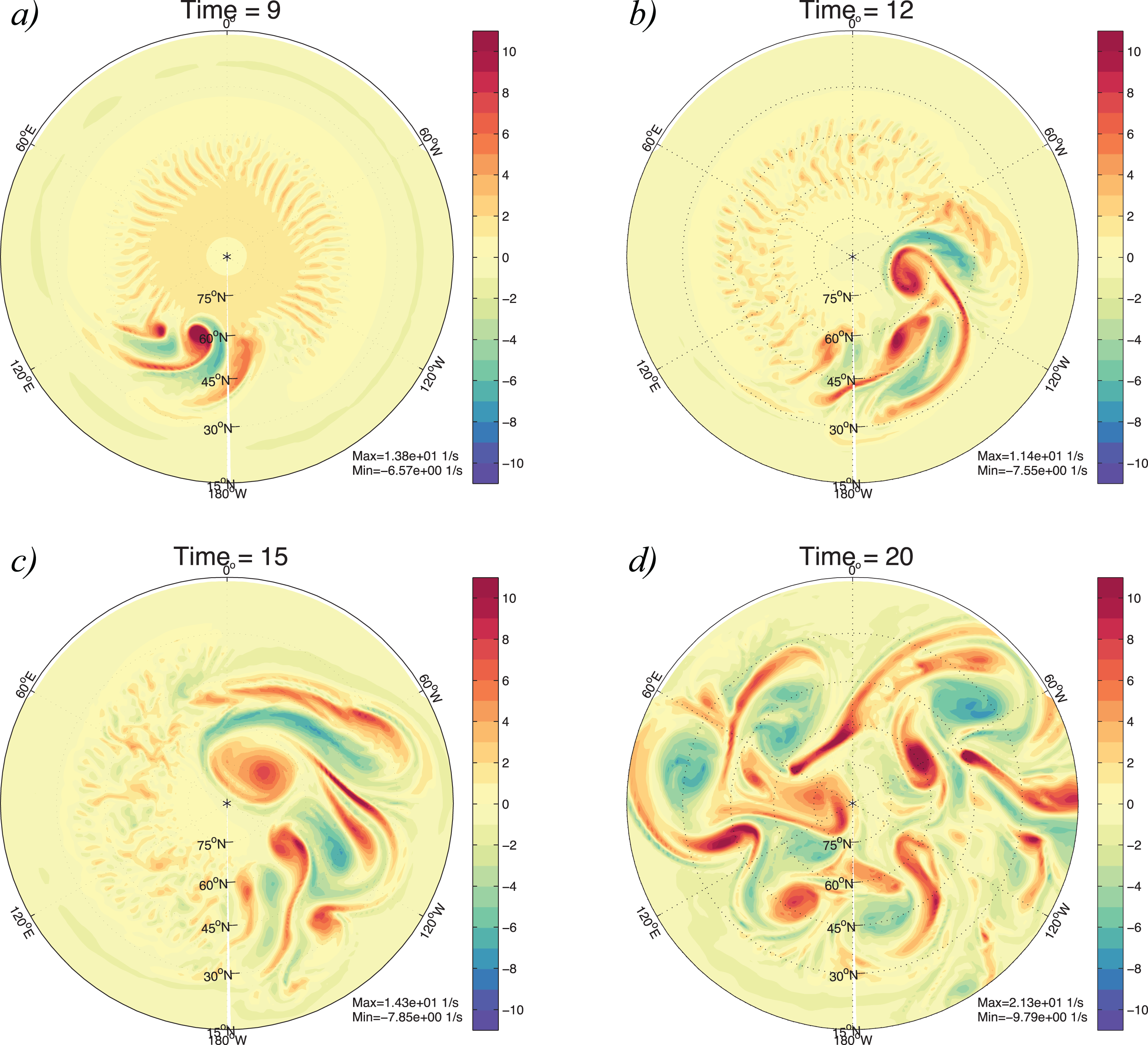
Baroclinic instability simulation at 9, 12, 15, and 20 days using a horizontal resolution of 50 km and a vertical resolution of 1 km. Shown is a top-view looking down onto the northern hemisphere. Plotted is the vertical component of the vorticity
The other test case is a 3-D rising thermal bubble in a box of 1000 m in each direction. This test case is initialized with a temperature perturbation in a neutrally stratified atmosphere. The precise definition and analysis of the full simulation is reported by Kelly and Giraldo (2012).
Both test cases are important for NWP applications. Operational weather prediction needs to cover the global circulation on the entire Earth like in the baroclinic wave test case. In order to use a higher resolution, for specific localized features of the atmosphere like hurricanes, one needs to run the simulation in limited area mode like in the 3-D rising thermal bubble test case.
4. Mesh generation and load balancing
The data structures and algorithms for parallel mesh generation, partitioning, and load balancing used in our simulations were provided by the p4est library. The p4est library has been used for efficient and scalable parallel adaptive mesh refinement for 2-D advection on the sphere (Burstedde et al., 2014), in other applications such as mantle convection and seismic wave propagation (Burstedde et al., 2010), and as a backend for the deal.II finite element library (Bangerth et al., 2015). Our present article is the first time that p4est is used for full 3-D atmospheric simulations. This article does not make use of the adaptive mesh refinement but it uses the p4est library to generate the grid for the simulations. This approach makes it possible to easily add adaptive mesh refinement in future work.
The p4est library represents 2-D and 3-D domains via a two-level structure, with a macro mesh and a micro mesh. The macro mesh is a conformal quadrilateral or hexahedral mesh, which is encoded as an unstructured mesh that is reproduced on each MPI process. Each element in the macro mesh is then treated as the root of a partitioned quadtree or octree, which recursively refines the macro element isotropically to create a micro mesh. The tree structure is represented in memory as a list of the leaves of the tree, ordered by the Morton curve (also known as the z-curve). This ordering induces a space filling curve that visits the centers of the leaves; while this curve is not a continuous space filling curve, it has many of their nice properties. One important property is that partitioning a domain by dividing the Morton curve into continuous segments creates subdomains that are fairly compact, with low surface-to-volume ratios (Hungershöfer and Wierum, 2002). This means that partitioning by this method keeps the intra-process communication during simulations low. A full description of p4est’s forest-of-quadtree and forest-of-octree data structures and algorithms can be found in the study by Burstedde et al. (2011).
When used in its raw form, the neighborhood information of an element in the micro mesh (i.e. which elements are adjacent) takes
The numerical methods in our simulations involve 3-D computations, but the vertical direction is treated differently from the other two: its grid resolution requirements are different, and achieving efficiency in the IMEX time evolution scheme (and other calculations that are performed only in the vertical direction) requires that vertical columns of elements and degrees of freedom be contiguous in memory. A forest-of-octrees approach would be ill-suited for these constraints. First, octree refinement is isotropic: the aspect ratio of a macro element is inherited by all of the micro elements created by refinement. This means that the relationship between horizontal and vertical resolution would have to be respected at the macro mesh level, increasing the macro mesh’s complexity. Second, the 3-D Morton curve does not respect the need to keep vertical columns contiguous: elements in a column would be separated in memory and, without care, would even be placed in separate partitions.
For these reasons, we want to use a forest-of-quadtrees approach to generate and partition vertical columns but to handle the elements within each column using a different approach. An extension to the p4est library, which was first used in the context of ice sheet modeling (Isaac et al., 2015b), provides the necessary data structures and interface. This extension is a set of “p6est” data types and functions (so named because it uses aspects of the 2-D “p4est” interface and the 3-D “p8est” interface). Essentially, it treats each vertical column as a list, from the bottom to top, of the elements created by recursive bisection of the full column and uses the existing 2-D p4est routines to manage the partitioning of columns and intercolumn interactions. A more complete description of this approach can be found in the study by Isaac (2015: Ch. 2). The p6est mesh format is illustrated in Figure 3.
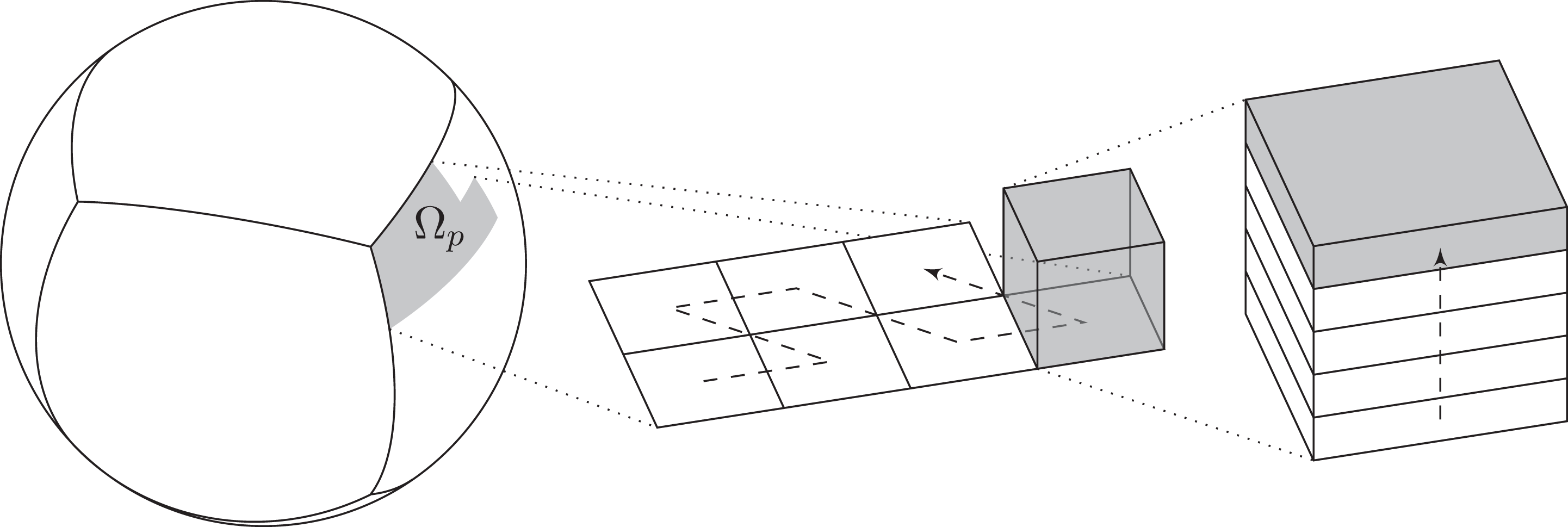
An illustration of meshing with the p6est extension of the p4est library. A macro mesh represents the cubed-sphere domain (left), division of the Morton curve creates the partitions for each MPI process, the columns in the
As the elements within a column are defined by recursive bisection, p6est was designed for meshes with
It should be noted that, although mesh adaptivity is not used in this work, the p6est data structures support bimodal local mesh adaptivity: elements may be independently refined in the vertical direction, and each column can be independently refined into four smaller columns.
5. Blue Gene/Q Mira
The simulations presented in this article were performed on the supercomputer Mira of the Argonne National Laboratory. Mira is an IBM BG/Q system offering 49,152 computational nodes. Each of these nodes has 16 cores resulting in a total number of 786,432 cores. Each core has a quad floating point unit. This permits running up to four MPI processes or up to four OpenMP (OMP) threads on each core. The maximum total number of hardware threads is therefore 3,145,728.
Important for the performance of our code is the memory architecture of Mira. Each computational node has 16 GB of random access memory (RAM). The processor receives its data from RAM through two levels of cache. Each core has its own level 1 (L1) cache of 16 KB, while the L2 cache of Mira is shared among all 16 processors of the computational node and has a size of 32 MB.
In addition to these two levels of cache, each core has an L1 cache prefetch (L1P) of 4 KB (Chung et al., 2012). Whenever the data needed for the simulation cannot be found in the L1 cache (L1 cache miss), the computer checks if this data are available in L1P. This is always done for an entire cache line of 128 bytes (16 double precision floating point numbers). If the requested cache line is not in L1P, it goes on and looks in L2 cache and eventually in the RAM for this data. The prefetcher of the BG/Q keeps track of previous cache misses. The stream prefetcher of the BG/Q establishes a stream if consecutive cache lines are requested, that is, L1P loads the next cache lines even when no cache miss occurs. If this consecutive data are actually needed by the code, this can save a lot of runtime. However, if the data are not used consecutively by the code, the prefetcher will read a lot of data from L2 cache without ever using it. This can produce a huge number of unnecessary cache misses.
Important for our optimizations is also the vector unit. The registers of Mira have a length of 256 bits offering space for four double precision floating point numbers. This allows performing up to eight double precision fused multiply-add floating point operations per core within the same clock cycle. Each core can perform one floating point instruction and one integer instruction per clock cycle. Load and store instructions take each one cycle of the integer unit.
6. Performance model
Making a theoretical performance model allows us to estimate the expected performance and to compare different numerical methods without fully optimizing them in our code. We created the performance model by counting all floating point operations as well as memory read and write accesses throughout our entire code. The optimal runtime is then computed by using the roofline model for the arithmetic intensity of the counted values. The results of this theoretical model are presented in Tables 1 to 3. We do this for three possible implementations: our CG version avoids having multiple copies of data in memory wherever possible (as in Figure 1(b)). The only variables that still require multiple values at the same physical locations are the metric terms in equation (5). The CG/DG version uses the same approach like the CG version for dynamically changing variables but allows additional copies of the data at element boundaries (Figure 1(c)) for data related to the reference atmosphere that does not change throughout the simulation. The DG version allows multiple copies of the data along element interfaces (Figure 1(c)) for all variables.
Theoretical amount of floating point operations and memory traffic for the rising thermal bubble test case at polynomial degree

CG: continuous Galerkin; DG: discontinuous Galerkin; BG: Blue Gene.
aThe effect of random memory access for CG is not taken into account in these results. All the numbers given in this table are summed over the entire simulation on 768 BG/Q nodes. The simulations use an effective resolution of 1.30 m in x- and y-direction and an effective resolution of 0.89 m in z-direction which leads to a total number of
Like Table 1 but including an estimate for the effect of random memory access due to CG storage if the previously computed elements are no longer available in cache.

CG: continuous Galerkin; DG: discontinuous Galerkin.
Theoretical amount of floating point operations and memory traffic for the baroclinic instability test case.a

CG: continuous Galerkin; DG: discontinuous Galerkin.
aThese results are calculated for 972 BG/Q nodes. The simulations use an effective horizontal resolution of 21.3 km and an effective vertical resolution of 1.0 km which leads to a total number of
Table 1 shows the expected number of floating point operations and total memory read and write traffic throughout the entire simulation for the rising thermal bubble test case. The additional copies of data along the element interfaces in DG storage lead to a significant increase in the number of floating point operations as well as memory traffic and to a significant reduction of arithmetic intensity. Our results for arithmetic intensity show that all of our cases are memory bound (see roofline plots in Figure 5). The optimal runtime in Table 1 is the runtime that we expect if we manage to reach 100% of the theoretical peak memory bandwidth as given by the STREAM benchmark in the study by Morozov et al. (2013). The percentage of the theoretical peak performance of the processor is also given in Table 1 for this optimal runtime. Our CG-only version gives us the best performance in all of these results.
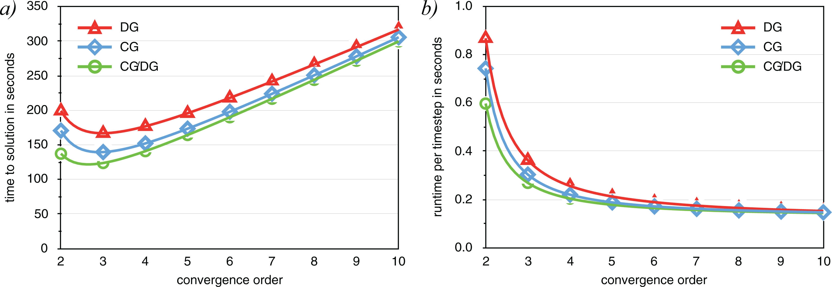
Time to solution (a) and runtime per time step (b) as a function of convergence order
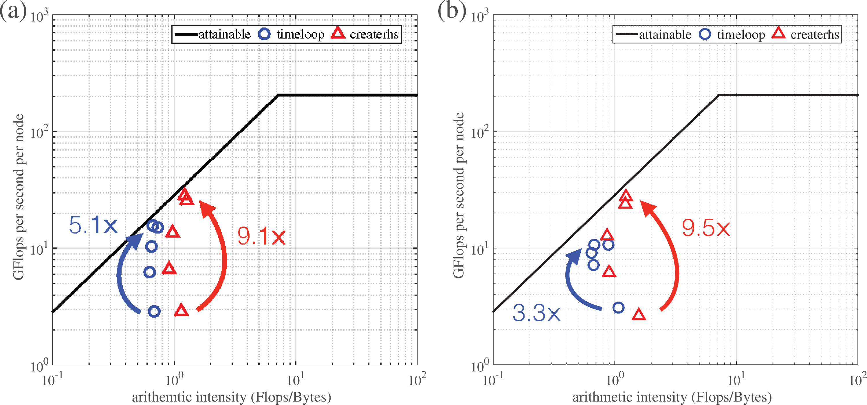
Roofline plot for the different versions shown in Tables 5 and 6 for (a) the rising thermal bubble test case and (b) for the baroclinic instability test case. For the identification of the different versions, we refer to the data in the tables. The arrows illustrate the performance improvement between the slowest and fastest version.
CG storage has a big disadvantage that we have not included in Table 1: we have to perform the computations of equation (5) on a per element basis while data stored in CG storage are not arranged on a per element basis. This leads to noncontiguous memory access that appears to be random. Having random memory access will not affect the results in Table 1 if most of the data is already in L2 cache. Therefore, the results of Table 1 will still be correct if the number of elements per compute core is small. Our goal for the rising thermal bubble problem is to use a very high grid resolution which produces much more data than we can fit into L2 cache. In this case, we expect to get a much better estimate for the performance of our code by assuming that none of the data is already in L2 cache and by counting the full cache lines in those cases where CG storage requires us to access only a small portion of that cache line. The results including this estimate for the effect of random memory access are shown in Table 2. Including the effect of random memory access does not change the number of floating point operations but it leads to a significant increase in memory traffic. This makes DG storage now the version with the highest arithmetic intensity and therefore the best percentage of the theoretical peak performance of the processes. The overall runtime of the entire simulation is still slower for DG storage due to the increased number of floating point operations. The winner in terms of overall runtime is our CG/DG version.
All of the results presented so far have been obtained for
Table 3 shows the results of our theoretical performance model for the baroclinic instability test case. As described in the introduction, our final goal is to run this test case at 3 km resolution on the entire supercomputer Mira. This setup gives us only 20 elements per hardware thread which makes it possible to fit most of the data in each time step into L2 cache. For this reason, we do not estimate the effect of random memory access in this case. Our CG and CG/DG versions are again significantly faster than our DG version. We will use the CG/DG version for our optimizations in the next section because this version gives us a significant advantage for the rising thermal bubble test case in Table 2.
7. Code optimizations
The goal of this section is to present the optimization steps of our CG storage version of NUMA for
Pseudocode of the main structure of our code NUMA. The part of the code highlighted in blue needs to be computed element-wise. The rest (black lines) can be computed for each grid point separately. MPI communication is highlighted in red.

We tried to optimize all parts of our code. We found create_rhs (the computation of the right-hand side in equation (4), see also Code example 1) to be the only function that contains enough floating point operations to allow significant optimizations.
Tables 5 to 8 show performance measurements for different versions of create_rhs. The different versions are explained in Table 4. For the rest of this section, we simply refer to the different versions in these tables. Versions MPI1 to OMP are measured by using the Hardware Performance Monitoring Toolkit. Version T gives theoretical expectations from our performance model as presented in the previous section. As in Table 2, we include here our estimate for random memory access for the rising thermal bubble test case. Version O is another theoretical result that is obtained by making some further optimizations. These optimizations consist of avoiding some unnecessary memory access and minimizing memory access by computing metric terms in equation (5) in each stage of our time integration method. This leads to a significant increase in the number of floating point operations but more importantly it allows a significant reduction in memory traffic. We will try these optimizations in our future work.

BG: Blue Gene; OMP: OpenMP.
aVersion PORT is the best portable version that we could achieve. Version BG/Q is the best version that we could get by using BG/Q vector instructions without OMP and version OMP is the best result with OMP. The versions T and O are theoretical results based on counting memory access by hand and estimating the runtime by using the memory bandwidth according to the STREAM benchmark results by Morozov et al. (2013).
Performance measurements for create_rhs (the computation of the right-hand side in equation (4), see also Code example 1) with the Hardware Performance Monitor Toolkit for the rising thermal bubble test case and the different versions of our code as described in Table 4.a

BG: Blue Gene; FMA: fused multiply-add.
aWe use the setup as described in Table 1. The column “runtime” shows the overall time spent in create_rhs (over all 690 time steps (3450 executions of create_rhs)). All measurements were obtained by taking the average values over four arbitrary nodes. We refer to the main text for the explanation of the other columns.
Performance measurements for the rising thermal bubble test case like in Table 5 but for the entire time loop.

BG: Blue Gene; FMA: fused multiply-add.

BG: Blue Gene; FMA: fused multiply-add.
Performance measurements for the entire time loop like in Table 6 but for the baroclinic instability test case.a

BG: Blue Gene; FMA: fused multiply-add.
aEven though only create_rhs is changed between the different simulations in this table, the runtime saved for the entire time loop is larger than the time saved in create_rhs. The reason for this behavior is that the reduced runtime of create_rhs leads to an improved synchronization between different MPI processes which reduces the time spent in MPI communication.
All of the measurements in Tables 5 to 8 are taken over the entire simulation. The column “% peak” gives the percentage of the theoretical peak performance of the processor. The column “% max.” shows how close this part of the code is to the maximum performance according to the roofline model for the given arithmetic intensity. The column “vect.” shows how many percent of all floating point operations are vectorized. The column “FMA” gives the percentage of fused multiply-add operations among all floating point operations. We have not estimated the optimal number of fused multiply-add operations in our performance model. For this reason, we leave the column “fma” empty for the versions T and O. The column “mix” shows the percentage of floating point instructions among all instructions.
We made simulations with a fairly high polynomial order of
We computed the derivatives of equation (5) in versions MPI1 and MPI4 for each of the five variables of
The rest of our optimizations can be categorized into three main topics which we discuss in the following subsections: compiler optimizations, BG/Q vector intrinsics, and OMP. At the end of this section, we give a short description of possible next steps for further optimization.
7.1. Compiler optimization
To improve the performance while retaining portability, we worked first on enabling better optimization through the compiler. We spent some time on finding the best level of compiler optimization for each function of our code. We found a few functions for which level 3 optimization gave us wrong results. This is not surprising because level 3 compiler optimization is not IEEE compliant.
Many of our operations in create_rhs looked initially like Code example 2. The operations were computed for each grid point of the element separately which makes it impossible for the compiler to vectorize the code. This explains the very low fraction of vectorized operations in versions MPI1 and MPI4 (column “vect.” in Tables 5 to 8).
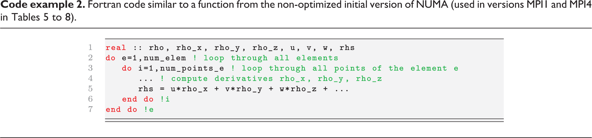
To improve vectorization, we changed our code in such a way that the operations are performed for the entire element at once (Code example 3). Our measurements for version PORT show that this simple modification leads to a significant improvement of the vectorization.
Like Code example 2 rewritten for improved compiler vectorization (used in version PORT).

7.2. BG/Q vector intrinsics
To make even better use of the vector unit, we rewrote our function create_rhs by using BG/Q vector intrinsics (Code example 4). This gave us another significant speedup (version BG/Q). This brings create_rhs to an excellent level of about 80% of the maximum attainable performance according to the roofline model (column “% max.” in Tables 5 and 7 and Figure 5).
Like Code example 2 rewritten with vector intrinsics (used in versions BG/Q and OMP).

Measurements showed that about 13% of all loads hit L2 cache and about 7% hit L1P. These fairly large numbers seem to be due to the random memory access that CG storage produces. Optimal would be if the prefetcher could bring all data into L1 cache before it is needed. We tried different prefetching strategies and handwritten prefetching but could not improve the performance compared to the default strategy. According to our performance model, we still expect CG storage to be significantly faster compared to DG storage even though CG storage makes prefetching very difficult.
7.3. OpenMP
OMP allows a reduction in the number of MPI processes. This leads for CG storage to a reduced amount of work for some parts of the code (namely the black text in Code example 1). However, we need to be very careful to avoid race conditions. In create_rhs, race conditions can occur in the summation over all the elements in equation (4). Using OMP atomic statements made our code too slow. The best solution that we could find was to reorder the elements inside each MPI process in such a way that different OMP threads can never compute neighboring elements at the same time. To ensure this, we need to synchronize all threads by using an OMP barrier after each element computation. These barriers slow down create_rhs by less than 10% (version OMP). Nevertheless, we obtain in the case of the baroclinic instability a noticeable improvement on the runtime of the entire simulation due to the reduced amount of work for the IMEX corrections in the vertical direction. We obtained the best performance by using 4 OMP threads per MPI process (2, 8, 16, and 64 OMP threads per MPI process were slower).
Comparing our final version OMP with our theoretical results (version T) shows reasonably good agreement (Tables 6 and 8). The number of floating point operations in our theoretical performance model has been tuned to agree with our overall measurements of version OMP in order to take compiler optimizations into account.
7.4. Next steps
The roofline plots in Figure 5 show that our optimizations have given us a massive improvement in the number of gigaflops per second per node which has brought us very close to the maximum attainable performance at the given arithmetic intensity. Our measurements show also that our final version OMP achieves an excellent level of vectorization (98.6% of all floating point operations are vectorized). The main remaining bottleneck of our optimized code is the low arithmetic intensity and the low instruction mix (Tables 5 to 8). As mentioned in Section 5, each load and store instruction takes one cycle of the integer unit. This explains the low instruction mix and demonstrates that our code could perform a lot more floating point operations while still achieving the same performance. In order to improve performance further, we need to increase arithmetic intensity by reducing the overall amount of memory traffic. We have found some unnecessary memory access which we will remove in our future work and we have found that we could reduce memory traffic by recomputing the metric terms in equation (5) in each stage of our time integration method. These optimizations have been included in our performance model and are shown in version O in Tables 5 to 8. According to our performance model, we should be able to achieve another factor 2 of speedup for create_rhs. This should bring us to about 35% of the theoretical peak performance of the processor. Recomputing the metric terms in each time integration stage should also improve the very low percentage of floating point instructions among all instructions (column “mix” in Tables 5 to 8). We will try these optimizations in our future work.
8. Strong scaling results
We present in this section strong scaling results up to the entire machine Mira for the baroclinic wave test case (Figures 6, 7, and 9) and the rising thermal bubble test case (Figures 8 and 10). All these results use version OMP from Section 7.
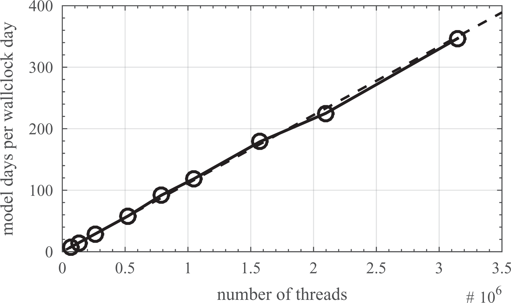
Strong scaling for the baroclinic wave test case with polynomial order
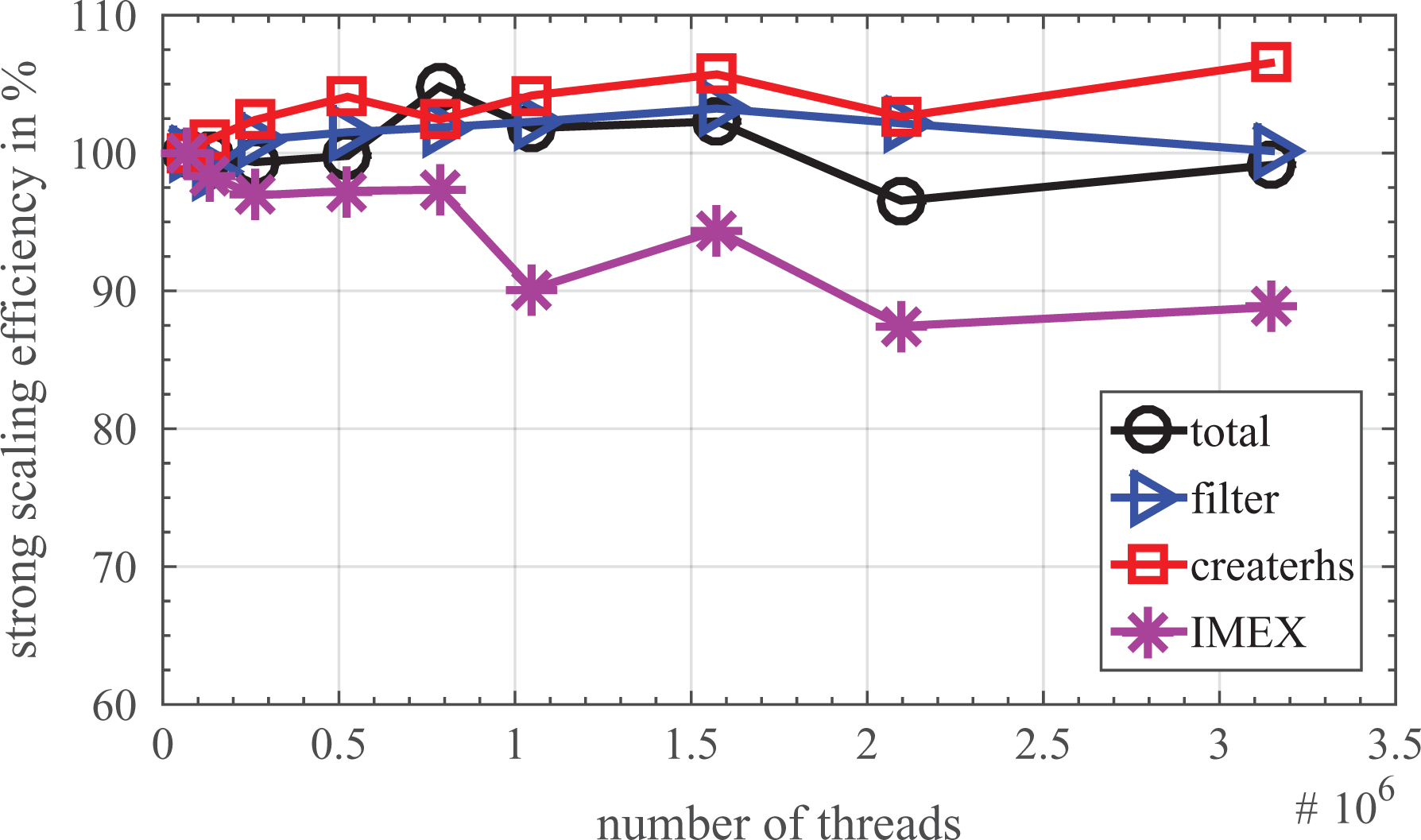
Strong scaling efficiency over base run on
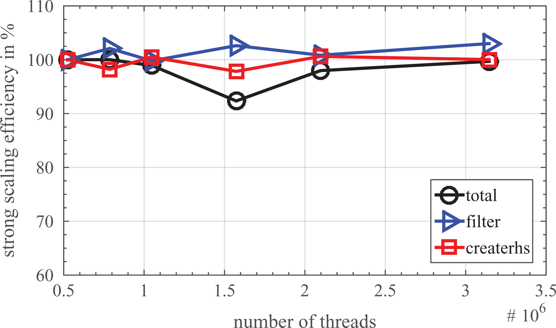
Strong scaling efficiency over base run on
The runtime of the entire simulation for the baroclinic wave test case is shown in Figure 6. The dynamics of a 1-day forecast needs to be finished within less than about 4.5 min runtime (more than 320 model days per wall clock day). We reach this goal on the entire machine Mira for our 3.0 km uniform horizontal resolution simulation of the baroclinic wave test case which takes 4.15 min runtime per 1 day forecast (346.6 model days per wall clock day).
The strong scaling efficiency of the simulations in Figure 6 is shown in Figure 7 for the different parts of the code. The entire code reaches a strong scaling efficiency of 99.1% on the entire machine Mira. The parts create_rhs and filter show a scaling efficiency of more than 100%. This is not surprising because the problem fits better into L2 cache with increasing number of threads and at the same time the time spent in our OMP barriers is decreasing. The IMEX part gives us the lowest scaling efficiency. We still need to understand the reason for this behavior.
The lowest scaling efficiency for the entire simulation is obtained for
The strong scaling efficiency of the rising thermal bubble test case is shown in Figure 8. We achieve 99.7% strong scaling efficiency on the entire machine for this case. We use a much larger total number of grid points of about 43 billion grid points for this case because we plan to use our code for hurricane and cloud simulations at this kind of problem size. We have not optimized the memory usage of our code. The smallest number of threads that can handle this problem is currently
The percentage of the theoretical peak performance in terms of floating point operations is shown in Figures 9 and 10. Not surprisingly, we obtain the best performance for our optimized part create_rhs. For the baroclinic wave test, create_rhs reaches 1.21 PFlops (12.1% of peak) and for the rising thermal bubble test, it reaches 1.28 PFlops (12.8% of peak) on the entire machine. The sustained performance of the entire simulation is at 0.55 PFlops for the baroclinic wave test and at 0.70 PFlops for the rising thermal bubble test on the entire machine Mira.
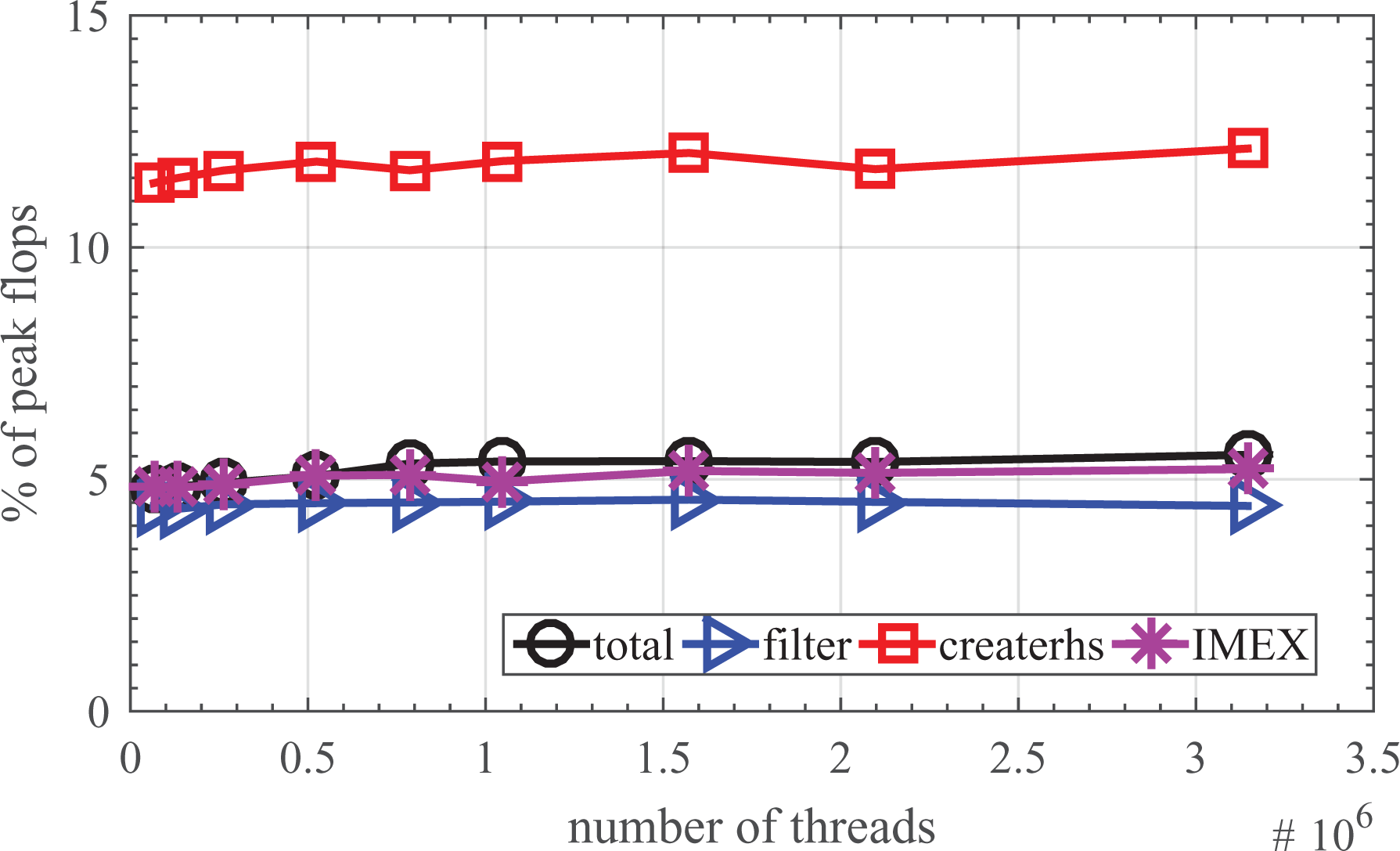
Percentage of theoretical peak performance in terms of floating point operations for the baroclinic wave test case like in Figure 6.

Percentage of theoretical peak performance in terms of floating point operations for the rising thermal bubble test case like in Figure 8.
9. Conclusions
In this article, we present the optimization and performance analysis of the atmospheric model NUMA. Our optimizations have improved the performance of the main computational kernel create_rhs of our code by a factor of almost 10 and have brought us very close to the maximum attainable performance due to the peak memory bandwidth (Figure 5). These optimizations allow us to perform most of the computations at 1.2 PFlops on the entire supercomputer Mira by using BG/Q vector intrinsics. The sustained performance of the entire simulation is at 0.70 PFlops for a rising thermal bubble test case using explicit time integration. We have not optimized all parts of the code yet. For the baroclinic wave test, the non-optimized computations for the implicit part of the time integration lead to a slightly lower sustained performance of 0.55 PFlops. We expect to improve our performance significantly by optimizing the remaining non-optimized parts of our code. The best portable version of the main computations was found to be about two times slower than the best non-portable version. We used the IBM XL compiler in this work. We expect the comparison between portable and non-portable optimizations to be very different on other architectures due to the availability of different compilers.
We have shown that NUMA achieves a near perfect strong scaling efficiency of 99.7% for the rising thermal bubble test case using 43 billion grid points on the entire 3.14 million threads of Mira. For the baroclinic wave test case on the sphere, we obtain a strong scaling efficiency of 99.1% using a mesh with 1.8 billion grid points. This allows us to compute a 1-day forecast at 3.0 km resolution within 4.15 min runtime and fulfils the requirements for operational weather prediction (less than 4.5 min runtime for the dynamics of a 1-day forecast).
As explained in the introduction, we expect this massive increase in resolution to be a major step toward more accurate weather forecasts. Nevertheless, the demand to increase the resolution of NWP models does not end at 3 km resolution (Bauer et al., 2015). The demand for better performance is even more severe when high resolution climate prediction is considered. Climate prediction requires forecast periods of more than 100 years. To simulate such a long period of time at a resolution of 3 km would still require about 1 year of runtime on the entire machine Mira when tracers and physics parameterizations are taken into account. For this reason, we need to continue to work on improving the performance of our code and to optimize it for next generation supercomputers.
Our analysis in this article shows that we need to reduce the amount of memory traffic to further improve our performance. It should be possible to achieve this by recomputing metric terms in each stage of our time integration method. For this reason, we expect to improve our sustained performance of the entire simulation beyond 1 PFlops. This should allow us to reach a uniform horizontal resolution close to 2 km within operational requirements. The next goal will be the optimization of our code for the upcoming next generation supercomputer Aurora at the Argonne National Laboratory. We hope to be able to reach 1 km resolution for global NWP once Aurora is available and once our code is fully optimized for that machine.
Footnotes
Authors’ note
Michal A Kopera is now affiliated to Department of Earth and Planetary Science, University of California, Santa Cruz, CA, USA.
Acknowledgements
The authors would like to thank Vitali Morozov at the Argonne National Laboratory for his support in analyzing the performance of our code with the Hardware Performance Monitor Toolkit. AM, MK, and SM are grateful to the National Research Council of the National Academies.
Declaration of Conflicting Interests
The author(s) declared no potential conflicts of interest with respect to the research, authorship, and/or publication of this article.
Funding
The author(s) disclosed receipt of the following financial support for the research, authorship, and/or publication of this article: This work was supported by the Office of Naval Research (PE-0602435 N), the Air Force Office of Scientific Research (Computational Mathematics program), and the National Science Foundation (Division of Mathematical Sciences; 121670). This research used resources of the Argonne Leadership Computing Facility, which is a DOE Office of Science User Facility supported under Contract DE-AC02-06CH11357.