Parallelization of the solve phase in a task-based Cholesky solver using a sequential task flow model

Abstract

We describe the parallelization of the solve phase in the sparse Cholesky solver SpLLT when using a sequential task flow model. In the context of direct methods, the solution of a sparse linear system is achieved through three main phases: the analyse, the factorization and the solve phases. In the last two phases, which involve numerical computation, the factorization corresponds to the most computationally costly phase, and it is therefore crucial to parallelize this phase in order to reduce the time-to-solution on modern architectures. As a consequence, the solve phase is often not as optimized as the factorization in state-of-the-art solvers, and opportunities for parallelism are often not exploited in this phase. However, in some applications, the time spent in the solve phase is comparable to or even greater than the time for the factorization, and the user could dramatically benefit from a faster solve routine. This is the case, for example, for a conjugate gradient (CG) solver using a block Jacobi preconditioner. The diagonal blocks are factorized once only, but their factors are used to solve subsystems at each CG iteration. In this study, we design and implement a parallel version of a task-based solve routine for an OpenMP version of the SpLLT solver. We show that we can obtain good scalability on a multicore architecture enabling a dramatic reduction of the overall time-to-solution in some applications.

Keywords

Sparse Cholesky backward substitution forward substitution SPD systems runtime systems OpenMP

1. Introduction

In this study, we are solving the linear system

A x = b

where A is a large sparse symmetric positive-definite matrix. In order to do this, we use a direct method where the solution process consists of three main steps: the analyse, the factorization and the solve phases. We use a Cholesky factorization given by

P^{T} A P = L L^{T}

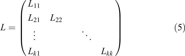
where L is a sparse lower triangular matrix, and P is a permutation matrix needed to preserve the sparsity. Since L is triangular, the solution can be obtained using a forward substitution step

L y = P b

followed by a backward substitution step

L^{T} z = y

so that $x = P^{T} z$ is the solution to the system in equation (1). Note that, although the factor L has a sparse structure, it is usually denser than A because of fill-in. The purpose of the analyse phase is to determine precisely the structure of L and to find a pivot order for limiting the fill-in. The returned permutation matrix P reduces the storage for the factor as well as the number of floating-point operations for factorization and solution.

In this article, we concentrate on the steps in equations (3) and (4). Most work on sparse solvers concentrates on the factorization in equation (2) because that is the most costly step of the solution process. As a consequence, the solve phase is often not as optimized as the factorization in the state-of-the-art solvers, and opportunities for parallelism are often not exploited in this phase. However, in some applications, the time spent in the solve phase is comparable to or even greater than the time for the factorization, and the user could dramatically benefit from a faster solve routine. This is the case, for example, for a conjugate gradient (CG) solver using a block Jacobi preconditioner. The diagonal blocks are factorized once only, but their factors are used to solve subsystems at each CG iteration.

Runtime systems such as StarPU (Augonnet et al., 2011), OpenMP and PaRSEC (Bosilca et al., 2013) provide a high-level API for implementing task-based algorithms where the directed acyclic graph (DAG) of tasks can be represented using different models. The most user-friendly model is the sequential task flow (STF) supported by the vast majority of runtime systems. Alternative models include the parametrized task graph (PTG) model supported by only a few runtime systems such as PaRSEC. Although the PTG model can offer some benefits in terms of performance over the STF model, it is generally much more difficult to use in practice especially in the context of sparse algorithms where the task dependency pattern is very irregular.

When using runtime systems, the runtime system is responsible for handling the DAG on the target architecture by managing the data dependencies, data coherency and task scheduling. One main advantage of this compared to using low-level synchronization mechanisms lies in the fact that it offers better portability and maintainability of the code. Furthermore, we conducted extensive experiments on using runtime systems in previous work for a sparse Cholesky factorization. We used both the STF model (Duff et al., 2018) and the PTG model (Duff and Lopez, 2018), in the context of the SpLLT solver, and we showed it was efficient in terms of performance when running on multicore architectures compared to the state-of-the-art solver HSL_MA87 from the Harwell Subroutine Library (HSL) (http://www.hsl.rl.ac.uk/).

In this article, we extend our approach to the solve phase in SpLLT and design DAG-based algorithms for implementing the parallel version of the forward and backward substitutions. Our implementation relies on an STF model, and the parallelization is achieved using the tasking features available in the OpenMP standard. We experimentally show that, using our DAG-based approach, we are able to obtain much better performance for computing the forward and backward substitutions on multicore architectures compared to the state-of-the-art solvers PARDISO, PaStiX and HSL_MA87.

In Section 2, we discuss the solve phase for dense systems, since we will use similar kernels in our sparse solve phase. We then describe the sparse solve algorithm in Section 3 before considering how to implement this in parallel in Section 4. We present our experimental results in Section 5 where we illustrate the scalability both with respect to the number of cores and to the number of right-hand sides (nrhs). We also compare our code with other state-of-the-art codes. Finally, we present some conclusions in Section 6.

2. DAG-based dense forward and backward substitutions

In this section, we discuss in detail the forward and backward substitutions for the case of dense matrices. For the sake of clarity and without loss of generality, we do not include the permutation matrix in this section. When performing these operations, we first partition the lower triangular dense factor $L \in ℝ^{n \times n}$ into blocks as:

L = (\begin{matrix} L_{11} \\ L_{21} & L_{22} \\ ⋮ & ⋱ \\ L_{k 1} & L_{k k} \end{matrix})

where $L_{i i} \in ℝ^{n b \times n b}$ are lower triangular matrices for $1 \leq i < k$ , and $L_{k k}$ is also a square lower triangular matrix but with dimension $n - (k - 1) n b \leq n b$ .

We first discuss the forward substitution in Section 2.1 before considering the backward substitution in Section 2.2.

2.1. Forward substitution

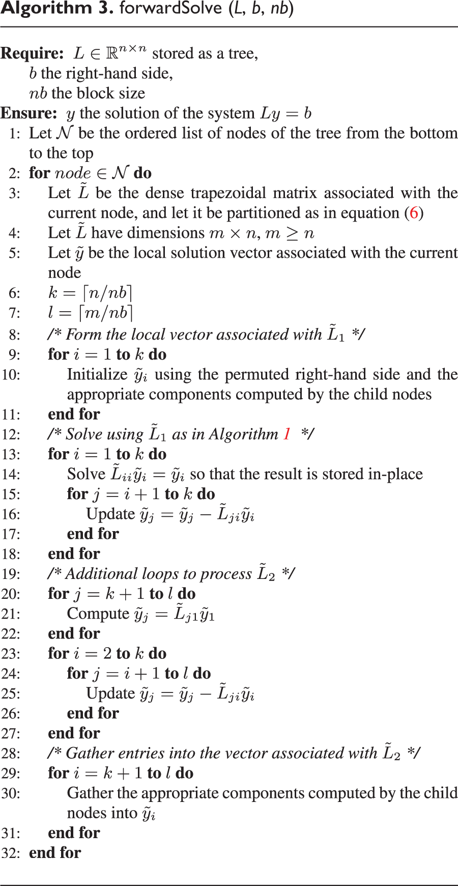
Consider first the forward substitution in equation (3) that we present in Algorithm 1.

Algorithm 1.

forwardSolve (L, b, nb)

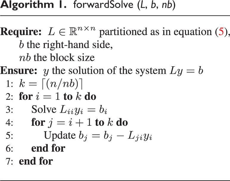
Algorithm 1 shows that the forward substitution requires two computational kernels. The first kernel at line 3 corresponds to the classical triangular solve, that is referred to hereafter as the solve kernel, denoted by dtrsv in the BLAS (Blackford et al., 2002). We note that the solve kernel is different from the above-mentioned solve phase and is indeed just part of this phase. The second kernel at line 5 is the update of the right-hand side by performing a matrix–vector product, which is referred to hereafter as the update kernel, dgemv in BLAS parlance.

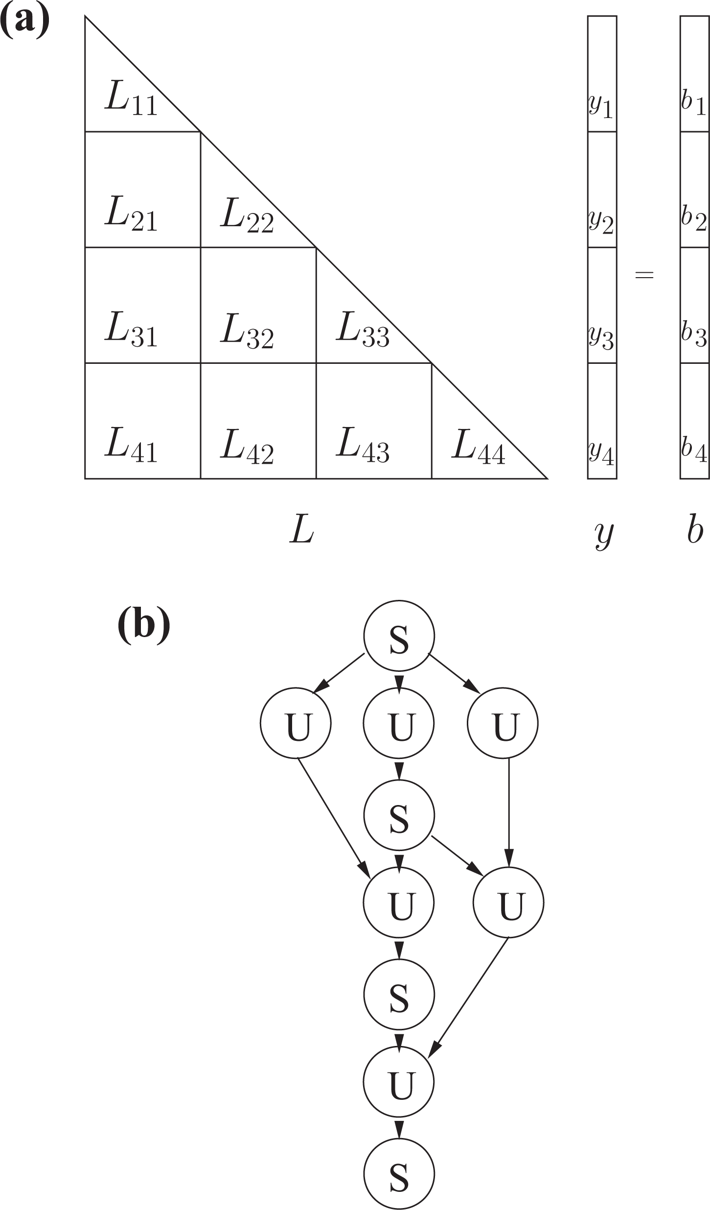
From Algorithm 1, we note that the update follows the solution of part of the right-hand side and triggers the solution of another part of b. That is, there is a dependency between the update and the solve. We can generate a DAG to show the dependencies in Algorithm 1. To illustrate this, we consider the case $k = 4$ and present the associated DAG in Figure 1(b).

Figure 1.

DAG associated with the forward solve on a partitioned L, as presented in Algorithm 1, with $k = 4$ . The nodes labelled S correspond to a call to the solve kernel (line 3), and the nodes labelled U correspond to a call to the update kernel (line 5). (a) Partitioned matrix and (b) associated DAG. DAG: directed acyclic graph.

The DAG starts by solving the equation $L_{11} y_{1} = b_{1}$ , represented by the top node S. Once, y ₁ is computed, an update of b can be performed. The updates to b ₂, b ₃ and b ₄ correspond to different parts of b, and they can all be performed in any order. The update of b ₃ using y ₁ and the update of b ₃ using y ₂ have to be completed before solving $L_{33} y_{3} = b_{3}$ . However, as the destination space is the same for both updates, these two operations cannot be performed at the same time. We see from the DAG in Figure 1(b) that some parallelism can be exploited in the updates to the right-hand side.

2.2. Backward substitution

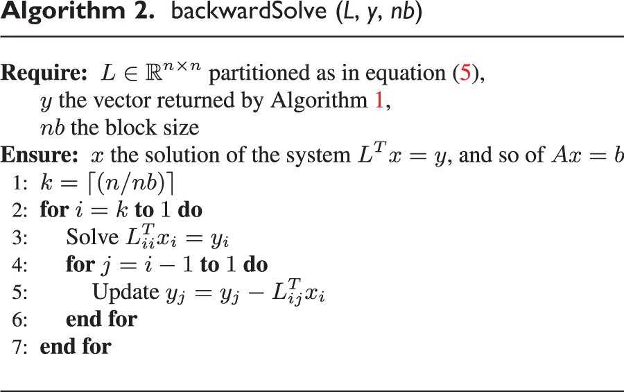
Once the forward substitution has returned the vector y, the solve phase performs a backward substitution to solve equation (4). In this equation, we use the transpose of L to compute the solution vector x. However, this substitution does not really differ from the previous one, only the loop order is changed, as shown in Algorithm 2. Similar to the forward substitution, this algorithm requires two computational kernels, the solve kernel and the update kernel, which give the same DAG as shown in Figure 1(b).

Algorithm 2.

backwardSolve (L, y, nb)

3. DAG-based solve in sparse case

In this section, we extend the algorithms presented in Section 2 to the sparse case. We now consider A as a sparse matrix of dimension n × n. The first step for solving equation (1) in SpLLT is the analysis of the pattern of the matrix A in order to reduce the fill-in in L during the factorization. This approach to solving sparse systems is well–documented, and we refer the reader to Duff et al. (2017) for the details. This step can use an ordering algorithm such as AMD (Amestoy et al., 1996) or Metis (Karypis and Kumar, 1998). The analysis then generates a tree representation for the factorization process. We first present the internal representation of the L factor in SpLLT and then discuss the design and implementation of the forward and backward substitutions.

3.1. Internal representation of the L factor

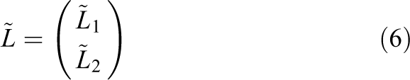
At the root node of the tree, that part of the L factor is held as a dense lower triangular matrix, and we will partition it as in equation (5). For the other tree nodes, the L factor is stored as a dense trapezoidal matrix, $\tilde{L}$ , that can be written as a square lower triangular matrix ${\tilde{L}}_{1}$ stacked over a rectangular matrix ${\tilde{L}}_{2}$ , namely

\tilde{L} = (\begin{matrix} {\tilde{L}}_{1} \\ {\tilde{L}}_{2} \end{matrix})

In the parlance of tree-based factorizations, the block ${\tilde{L}}_{1}$ corresponds to variables that are fully summed, that is to say variables that are appearing for the last time and do not appear at any ancestor nodes in the tree, so the corresponding unknowns can be solved as in Algorithm 1. The entries in ${\tilde{L}}_{2}$ are then used to perform updates to the variables that will later be fully summed at the parent or ancestor nodes of the tree. We can use these dependencies to generate a DAG for the whole solve phase that allows us to use inter-level parallelism. That is, a task at a node can be processed before some of the tasks for its children as long as the task has all its dependencies satisfied. We emphasize in passing two properties of the tree. Firstly, the rows within a block in ${\tilde{L}}_{2}$ may match rows of more than one block in the parent. Secondly, one row in the fully summed part of a node can be shared with more than one child node.

We illustrate this in Figure 2, where the factor L consists of three nodes. The parts of the DAG associated with the leaves of the tree are very similar to the DAG shown in Figure 1. We label the blocks from the leaves to the root. If there are rows in common between blocks $b l k_{7}$ and $b l k_{15}$ then there will be a dependency between y ₂ and y ₇. Moreover, we observe that there is at least one row present in all three nodes, so that the solve using the corresponding block in the parent node requires the updates from both the children. Note that the first solve task in the root node has no dependency with its children. The resulting internode parallelism means that the solve of the corresponding part of the solution vector, y ₅, can be executed before the tasks at the child nodes complete.

Figure 2.

Tree representation of the sparse triangular factor L and its associated DAG for the forward solve. The matrix corresponding to each node is partitioned into blocks of size nb, as in equation (5). The nodes labelled S correspond to a call to the solve kernel (line 3), and the nodes labelled U correspond to a call to the update kernel (line 5). (a) Partitioned L matrix and (b) associated DAG. DAG: directed acyclic graph.

For efficient implementation of the forward substitution, we must modify Algorithm 1 to take account of three elements. Firstly, the L factor is spread over the nodes of the tree. Secondly, the shape of the $\tilde{L}$ associated with each node of the tree is trapezoidal, except for the root. Thirdly, ${\tilde{L}}_{2}$ is composed of rows that have discontinuous indices in L so that indirect addressing is required.

3.2. Dense kernels and data movement

Our construction of the tree representation of the factor L is such that the rows of a node may not correspond to contiguous entries in b. However, the computational kernels do not handle indirect addressing. This leads to data movement between the global vector and a local vector so that the data are contiguous in the local vector. Thus, a local vector is associated with each node of the tree and is split into two parts: the part associated with ${\tilde{L}}_{1}$ consists of a contiguous portion of the global solution vector, whereas the second part is a workspace. One way in which we avoid indirect addressing is to use the right-hand side vector permuted according to the pivot ordering. That is to say that, for the forward substitution, we work from the vector Pb in equation (3). Thus, the part of the vector corresponding to the triangular block ${\tilde{L}}_{1}$ will be contiguous in the global vector and so we can work directly on this when solving for the fully summed variables. We believe this to be a novel feature for the sparse solve phase. We do not actually permute the right-hand side prior to the forward substitution but only when the entries of the right-hand side are needed by the solve kernel.

3.2.1. Forward solve and forward update kernels

We illustrate the two parts of $\tilde{L}$ and the movement or equivalence of global and local vectors in Figure 3. As mentioned earlier, the part of $\tilde{y}$ corresponding to ${\tilde{L}}_{1}$ is identical to the appropriate part of the global vector so no indirect addressing is required. The remaining part of $\tilde{y}$ is a workspace local to the node. This workspace is related to the global vector through indirect addressing corresponding to row indices in the blocks of ${\tilde{L}}_{2}$ . The first part of the local vector is set with the appropriate entries of Pb. In addition, both parts of the local vector may require a gather operation with workspaces of the children of the node. That is, when a row of $\tilde{L}$ is present in a child of the node and the associated block in the child is processed, there is an update of the local vector of $\tilde{L}$ using some entries from the child workspace. In Figure 3, we show in the dark shaded areas the solution for the fully summed variables that involve the block ${\tilde{L}}_{1}$ with the blocks y_i and $y_{i + 1}$ computed in-place. Since ${\tilde{L}}_{2}$ is composed of rows whose indices in y are discontinuous, indirect addressing is required in order to map these components into the contiguous local vector. These are then used for computing the matrix vector product ${\tilde{L}}_{3 j} {\tilde{y}}_{j}$ , with $j = 1, 2$ , and the resulting vector is subsequently scattered directly into the parent local vector. This is also a novel feature of the code.

Figure 3.

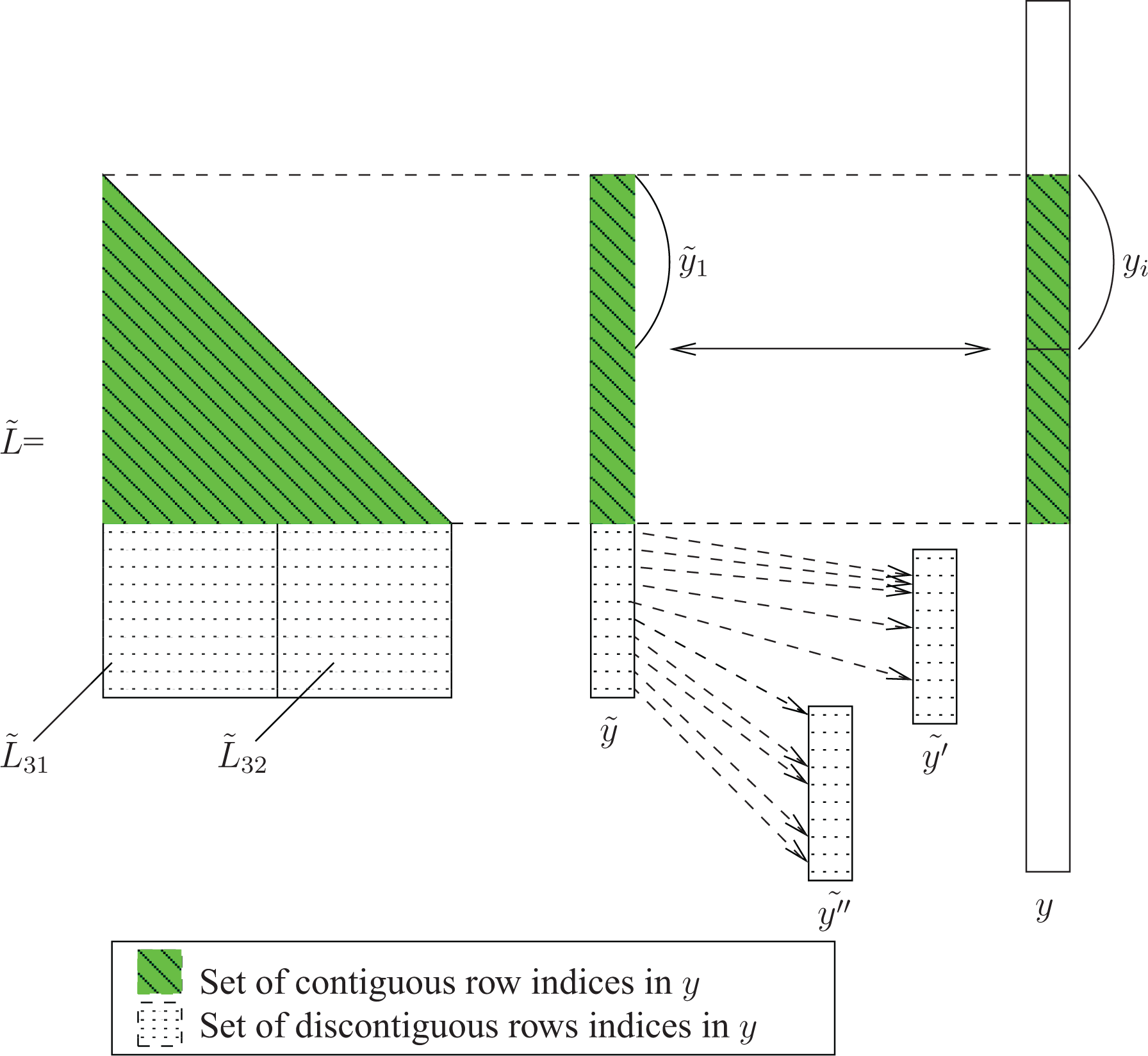
Data movement required by the computation of ${\tilde{L}}_{31} {\tilde{y}}_{1}$ and ${\tilde{L}}_{32} {\tilde{y}}_{2}$ during the forward solve of a node $\tilde{L}$ .

3.2.2. Backward solve and backward update kernels

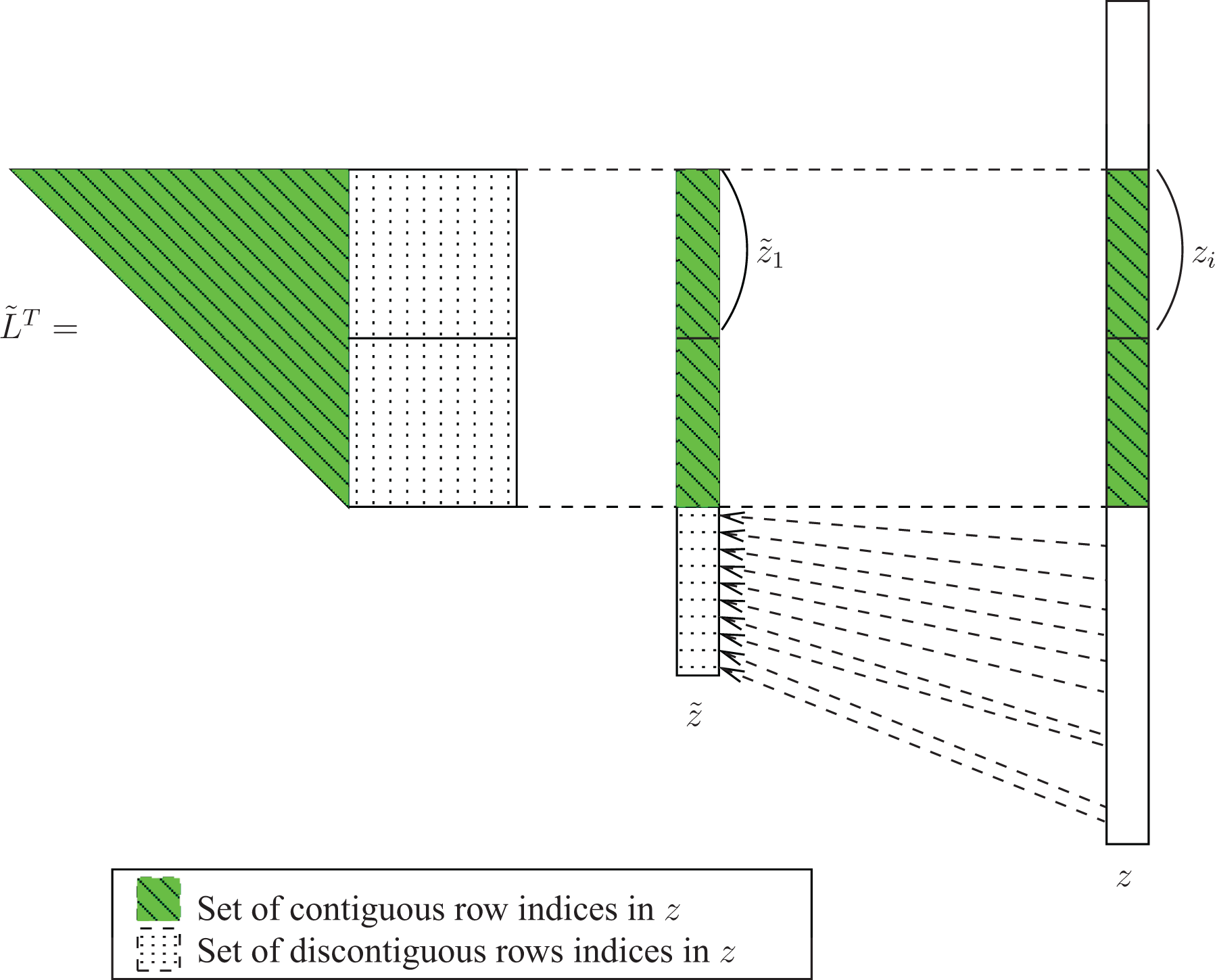
The backward substitution shares the same data locality issues as for the forward substitution. Consider the same node as in Figure 3 with its associated dense lower trapezoidal matrix $\tilde{L}$ . In order to update the solution vector $z = P x$ from equation (4) with ${\tilde{L}}_{2}^{T}$ , the backward update kernel has first to gather the corresponding components of z into a local vector, denoted by $\tilde{z}$ in Figure 4. Then, the update of z is performed by the computation of ${({\tilde{L}}_{31})}^{T} {\tilde{z}}_{3}$ and ${({\tilde{L}}_{32})}^{T} {\tilde{z}}_{3}$ . Each triangular solve computes part of Px. That is, the result of the triangular solve is then permuted to obtain the solution vector x.

Figure 4.

Data movement required by the computation of ${({\tilde{L}}_{31})}^{T} {\tilde{z}}_{3}$ and ${(L_{32})}^{T} {\tilde{z}}_{3}$ during the backward solve of a node $\tilde{L}$ .

3.3. Sequential sparse forward solve algorithm

Moving from the dense forward solve in Algorithm 1 to the sparse case requires several changes. Firstly, as shown in Figure 2, the L factor is now a tree, where the nodes are associated with trapezoidal matrices, and has internode dependencies. Secondly, as shown in Figures 3 and 4, processing ${\tilde{L}}_{2}$ leads to indirect addressing. We present the sequential sparse solve in Algorithm 3. This algorithm takes as input the same parameters as Algorithm 1, except that the representation of the factor L is a list of nodes of the tree. The forward substitution operates over the nodes from the leaves to the root of the tree. For each node, we have the associated dense matrix $\tilde{L}$ , as written in equation (6), and a local vector $\tilde{y}$ . We start by forming the part of $\tilde{y}$ associated with ${\tilde{L}}_{1}$ . That is, we gather the corresponding components of Pb with the contributions of the children of the node. This operation overwrites the content so that we avoid resetting the local vector. Then, ${\tilde{L}}_{1}$ is processed as in Algorithm 1. An additional loop is introduced in Algorithm 3 to process ${\tilde{L}}_{2}$ . This step is done so that the result of the first update of each ${\tilde{y}}_{j}$ , with $j \in {i + 1, \dots, l}$ , overwrites its content. Finally, we sum the contribution from the children to the local vector.

Algorithm 3.

forwardSolve (L, b, nb)

The backward substitution algorithm is very similar but, in this case, we use the L factor starting with the root node and working down the tree to the leaf nodes.

4. Parallel implementation of the solve phase

As mentioned in Section 1, the parallel implementation of our task-based algorithms, introduced Section 3, is achieved using a runtime system which is responsible for executing the DAG in parallel on the target architecture. This involves enforcing data dependencies to ensure the correctness of the execution and managing the task scheduling for efficiently exploiting the resources. This design strategy has the advantage of producing a code that is portable and easy to maintain.

For our implementation, we decide to rely on an STF model for its greater usability than the PTG model in the context of complicated algorithms such as sparse forward and backward substitutions. The difficulties for exploiting a PTG model compared to the STF model were exposed in previous work for the parallelization of the factorization phase in SpLLT (Duff and Lopez, 2018). The simplicity of the STF model lies in the fact that the parallel code is very similar to the sequential one. In this model, the tasks are submitted to the runtime system following the sequential algorithm and for each task, the manipulated data must be associated with a data access such as Read (R), Write (W) and Read–Write (RW) depending on the operations performed on the data. Using the task submission order and data access information, the runtime system is capable of building the DAG such that the sequential consistency is guaranteed during the parallel execution. Finally, we choose to use the OpenMP standard for our implementation, because we observed in previous work that it comes with a slightly lower overhead for the task management than a runtime system with many extra features such as StarPU (Duff et al., 2018).

In the following, we first show how the data dependency is determined using the representation of the factor L, and then, we describe the task management with OpenMP.

4.1. Data dependencies of a task

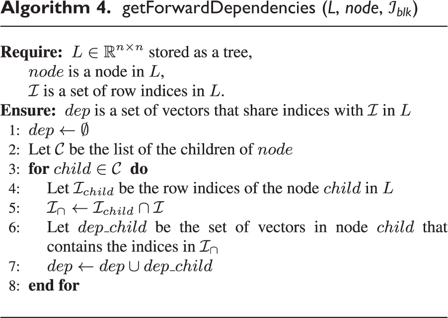
From the DAG as presented in Figure 2(b), we associate a task with a computational kernel that takes as input a block within a node of the tree and the related part of the input and output vector. The sparse aspect requires an additional task that handles the indirect addressing. This task forms the local vector by adding the contributions of the children. The submission of the tasks related to the forward substitution is presented in Listing 1. The computational operations within a node in Algorithm 3 are now considered as tasks that are submitted to the runtime system. We provide in addition the access mode to the data in each task to enable the runtime system to detect the dependencies between tasks.

Listing 1.

Task-based implementation of Algorithm 3.

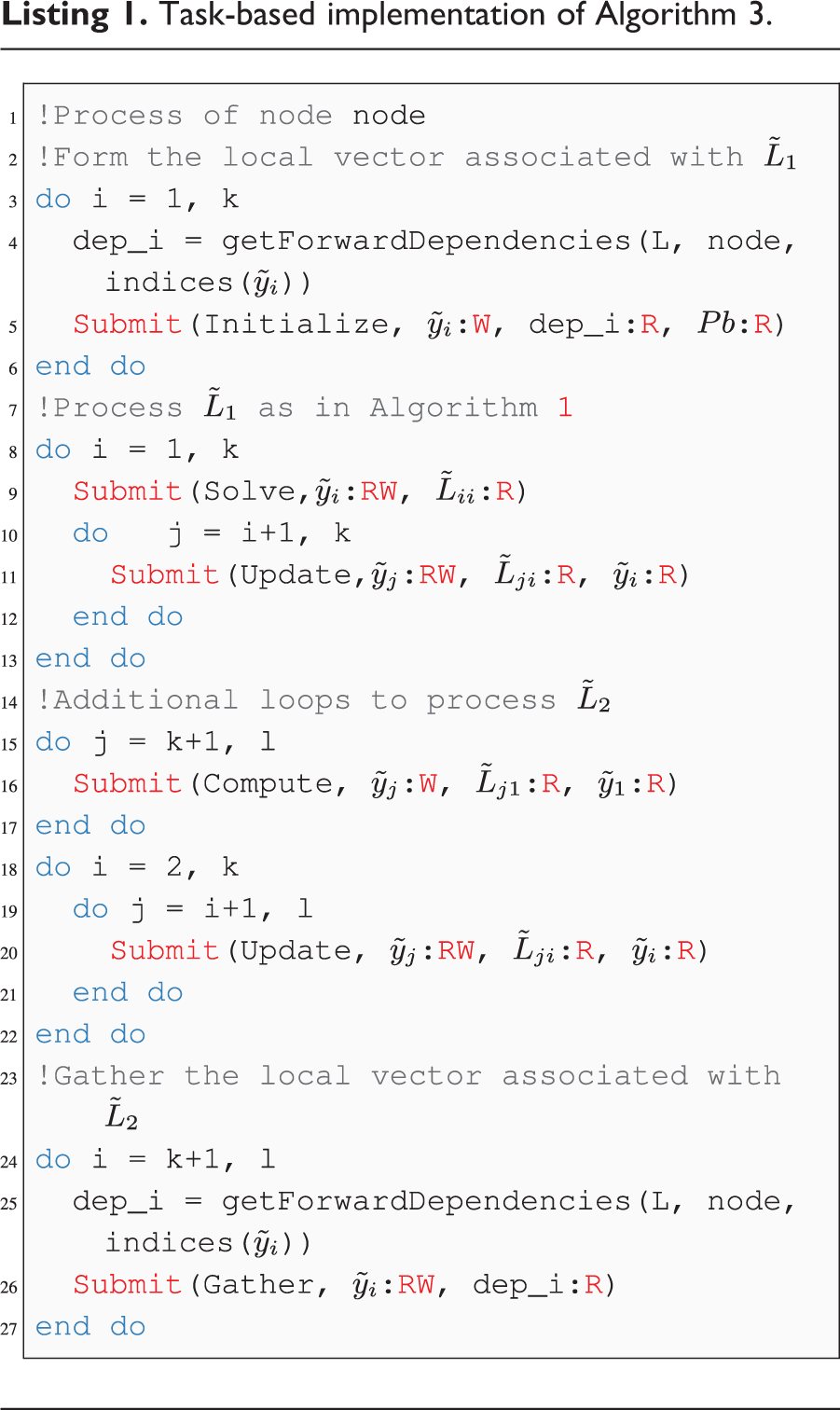
The data accessed local to a node, in lines 9, 11, 16 and 20, is similar to the dense case in Algorithm 1 and is independent of the pattern of the matrix. However, the sparse aspect requires gathering entries from a set of local vectors that share rows with the local vector, ${\tilde{y}}_{i}$ , of the node. We refer, hereafter, to this set as the data dependencies for ${\tilde{y}}_{i}$ , denoted by $d e p_{i}$ . Once the data dependencies are computed in line 4, a task is submitted in line 5 that overwrites ${\tilde{y}}_{i}$ with the appropriate part of Pb added to the contributions coming from the vectors in dep_i. On the other hand, in line 26, the submitted task modifies ${\tilde{y}}_{i}$ by gathering the contributions coming from the vectors in $d e p_{i}$ obtained in line 25.

We show how $d e p_{i}$ is computed in Algorithm 4. As in lines 4 and 25 of Listing 1, the initial parameters are the row indices of ${\tilde{y}}_{i}$ and the node that owns it. This algorithm creates dep by visiting the children of the node in line 3. For each child node of node, the part of the local vector that shares at least one row index with ${\tilde{y}}_{i}$ is considered as a data dependency. Note that, in practice, we compute this list once before the solve, and we use the list during the forward and backward substitutions. This saves computations when the solve phase is done multiple times.

Algorithm 4.

getForwardDependencies (L, node, $I_{b l k}$ )

The submission of the tasks for the backward substitution is similar to the forward substitution, except for the computations of the data dependencies, where the role of child nodes is replaced by the ancestor nodes.

4.2. Management of the tasks

Our implementation uses the runtime system OpenMP, Release 4.5. This release offers a runtime system that schedules the execution of tasks with dependencies. There are several ways to describe the dependencies. One simple way is to provide the address of the data that are being accessed through a read, write or read/write mode as in Listing 1. Thus, the dependencies have to be known at compilation time by OpenMP. However, the set dep returned by Algorithm 4 has a variable length and its length cannot be predicted prior to the execution of the code.

To handle a variable length of dependencies in OpenMP, we use a k-ary tree combined with synchronization tasks to control the scheduling of the task. A synchronization task is a task submitted to the runtime system that does nothing, like a no-op instruction, except to release a dependency for further use. The purpose of using a k-ary tree is to reduce the number of tasks from $N = | d e p |$ to c, an acceptable number of dependencies, given that we have to statically define each possibility in our code. To do this, we define a chunk, that is, a subset of unsatisfied dependencies, equal to c. The k-ary tree is processed as follows. At the first level of the k-ary tree, the dependencies in dep are considered to be unsatisfied and are split into $⌈ N / c ⌉$ chunks. For each chunk, a synchronization task is submitted to the runtime system. This synchronization task is scheduled when all dependencies in the chunk are satisfied. It then releases the first dependency of the chunk for the next level by flagging it as unsatisfied. Thus, the k-ary reduction leads to at most c unsatisfied dependencies, as presented in Figure 5. In this example, the size of the chunk is 5, and $N = 35$ . A white square represents an unsatisfied dependency, and a grey rectangle represents a set of satisfied dependencies. The first dependency of each chunk is still unsatisfied between two levels. A task is finally submitted to the runtime system with a list of dependencies composed of the remaining unsatisfied dependencies of dep.

Figure 5.

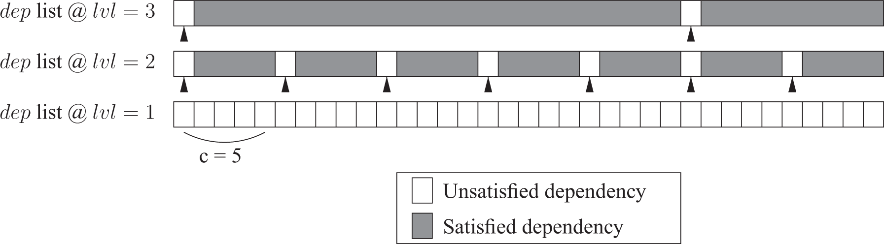
Content of the set dep at each level of the k-ary tree, with a chunk size $c = 5$ . Each white square represents a dependency in dep, and each grey rectangle is composed of dependencies already satisfied.

Along with this k-ary tree, we use a case statement over the number of unsatisfied dependencies in dep, where each case corresponds to the submission of a (synchronization) task having i dependencies ( $0 \leq i \leq c$ ), where c is 10 by default.

4.3. The pruning strategy

It is worth noting that the matrix sizes in the tree can vary significantly between the nodes of the tree. More specifically, the matrices are generally small near the leaf nodes and get bigger as we traverse the tree toward the root node. As a consequence, there is plenty of inter-level parallelism at the bottom of the tree with limited opportunity for intra-node parallelism. On the other hand, there is much less inter-level parallelism near the top of the tree, where there is much more intra-node parallelism. In our task-based algorithm, this would result in the creation of many small granularity tasks at the bottom of the tree which can be costly for the runtime system to manage compared to the actual workload being performed in these tasks. In addition, inter-level parallelism at the bottom of the tree can greatly exceed the amount of available resources. Therefore, a large number of tasks is generated at this level, increasing the cost for the task scheduling without bringing much benefit in terms of performance. In order to alleviate these problems, we employ a tree pruning strategy, largely inspired by the one used in the qr_mumps solver and described in the work of Buttari (2012). This allows us to dramatically reduce the number of small granularity tasks in the DAG. This pruning strategy aims at identifying a set of subtrees which are processed as a single task meaning that each subtree is processed in serial mode.

In more detail, the pruning algorithm performs a top-down traversal of the tree and selects a sufficiently large set of independent nodes in the tree so that the computational weight of the subtrees rooted at each node in this set is balanced. In practice, we force the number of subtrees to be equal to at least twice the number of resources, because we want to generate enough parallelism to compensate for potential load imbalance during the execution of the subtree within the whole DAG. One potential source of imbalance is that the metric used for estimating the computational weight for each subtree, the number of floating-point operations, might not accurately reflect the execution time.

This pruning strategy allows us to dramatically reduce the number of tasks submitted to the runtime system as well as the number of dependencies in the DAG. Moreover, processing the subtrees as a single task improves the exploitation of data-locality which increases the kernel efficiency.

5. Experimental results

In order to assess the performance of the solve phase of our SpLLT code, we ran tests on a set of 37 symmetric definite positive matrices, presented in Table 1. These matrices come from the Suitesparse matrix collection Davis and Hu (2011) and are those used in the work of Duff et al. (2018) and Hogg et al. (2010). They correspond to a wide range of different applications including computational fluid dynamics (CFD), circuit simulation, finite element modelling (FEM) and gas reservoir modelling. The dimensions of the matrices range from $36 \times 10^{3}$ to $1.5 \times 10^{6}$ . We focus our experiments on parallel efficiency both when nrhs increases and when the number of workers (nworker) increases. We also compare the performance of the SpLLT solve phase with the solve phase of other sparse direct solvers. Note that in the following tables, fastest time are in bold.

Table 1.

Test matrices and their characteristics without node amalgamation.^a

#		n ( $10^{3}$ )	nz (A) ( $10^{6}$ )	nz (L) ( $10^{6}$ )	Flops ( $10^{9}$ )	Application/description
1	Schmid/thermal2	1228	4.9	51.6	14.6	Unstructured thermal FEM
2	Rothberg/gearbox	154	4.6	37.1	20.6	Aircraft flap actuator
3	DNVS/m_t1	97.6	4.9	34.2	21.9	Tubular joint
4	Boeing/pwtk	218	5.9	48.6	22.4	Pressurized wind tunnel
5	Chen/pkustk13	94.9	3.4	30.4	25.9	Machine element
6	GHS_psdef/crankseg_1	52.8	5.3	33.4	32.3	Linear static analysis
7	Rothberg/cfd2	123	1.6	38.3	32.7	CFD pressure matrix
8	DNVS/thread	29.7	2.2	24.1	34.9	Threaded connector
9	DNVS/shipsec8	115	3.4	35.9	38.1	Ship section
10	DNVS/shipsec1	141	4.0	39.4	38.1	Ship section
11	GHS_psdef/crankseg_2	63.8	7.1	43.8	46.7	Linear static analysis
12	DNVS/fcondp2	202	5.7	52.0	48.2	Oil production platform
13	Schenk_AFE/af_shell3	505	9.0	93.6	52.2	Sheet metal forming
14	DNVS/troll	214	6.1	64.2	55.9	Structural analysis
15	AMD/G3_circuit	1586	4.6	97.8	57.0	Circuit simulation
16	GHS_psdef/bmwcra_1	149	5.4	69.8	60.8	Automotive crankshaft
17	DNVS/halfb	225	6.3	65.9	70.4	Half-breadth barge
18	Um/2cubes_sphere	102	0.9	45.0	74.9	Electromagnetics
19	GHS_psdef/ldoor	952	23.7	144.6	78.3	Large door
20	DNVS/ship_003	122	4.1	60.2	81.0	Ship structure
21	DNVS/fullb	199	6.0	74.5	100.2	Full-breadth barge
22	GHS_psdef/inline_1	504	18.7	172.9	144.4	Inline skater
23	Chen/pkustk14	152	7.5	106.8	146.4	Tall building
24	GHS_psdef/apache2	715	2.8	134.7	174.3	3D structural problem
25	Koutsovasilis/F1	344	13.6	173.7	218.8	AUDI engine crankshaft
26	Oberwolfach/boneS10	915	28.2	278.0	281.6	Bone micro-FEM
27	ND/nd12k	36.0	7.1	116.5	505.0	3D mesh problem
28	ND/nd24k	72.0	14.4	321.6	2054.4	3D mesh problem
29	Janna/Flan_1565	1565	59.5	1477.9	3859.8	3D mechanical problem
30	Oberwolfach/bone010	987	36.3	1076.4	3876.2	Bone micro-FEM
31	Janna/StocF-1465	1465	11.2	1126.1	4386.6	Underground aquifer
32	GHS_psdef/audikw_1	944	39.3	1242.3	5804.1	Automotive crankshaft
33	Janna/Fault_639	639	14.6	1144.7	8283.9	Gas reservoir
34	Janna/Hook_1498	1498	31.2	1532.9	8891.3	Steel hook
35	Janna/Emilia_923	923	21.0	1729.9	13,661.1	Gas reservoir
36	Janna/Geo_1438	1438	32.3	2467.4	18,058.1	Underground deformation
37	Janna/Serena	1391	33.0	2761.7	30,048.9	Gas reservoir

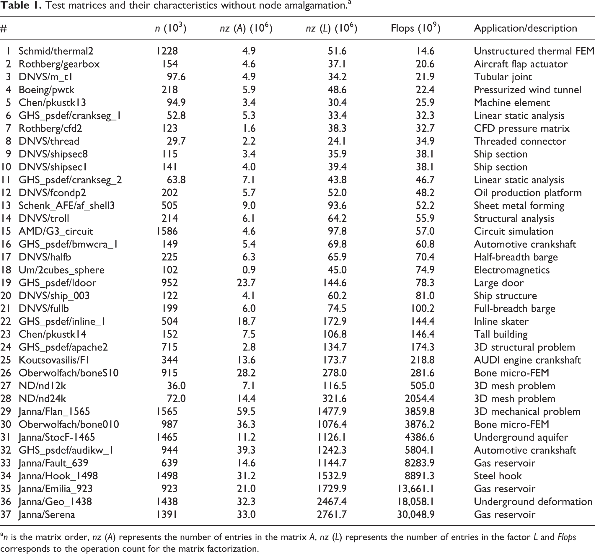
^a n is the matrix order, nz (A) represents the number of entries in the matrix A, nz (L) represents the number of entries in the factor L and Flops corresponds to the operation count for the matrix factorization.

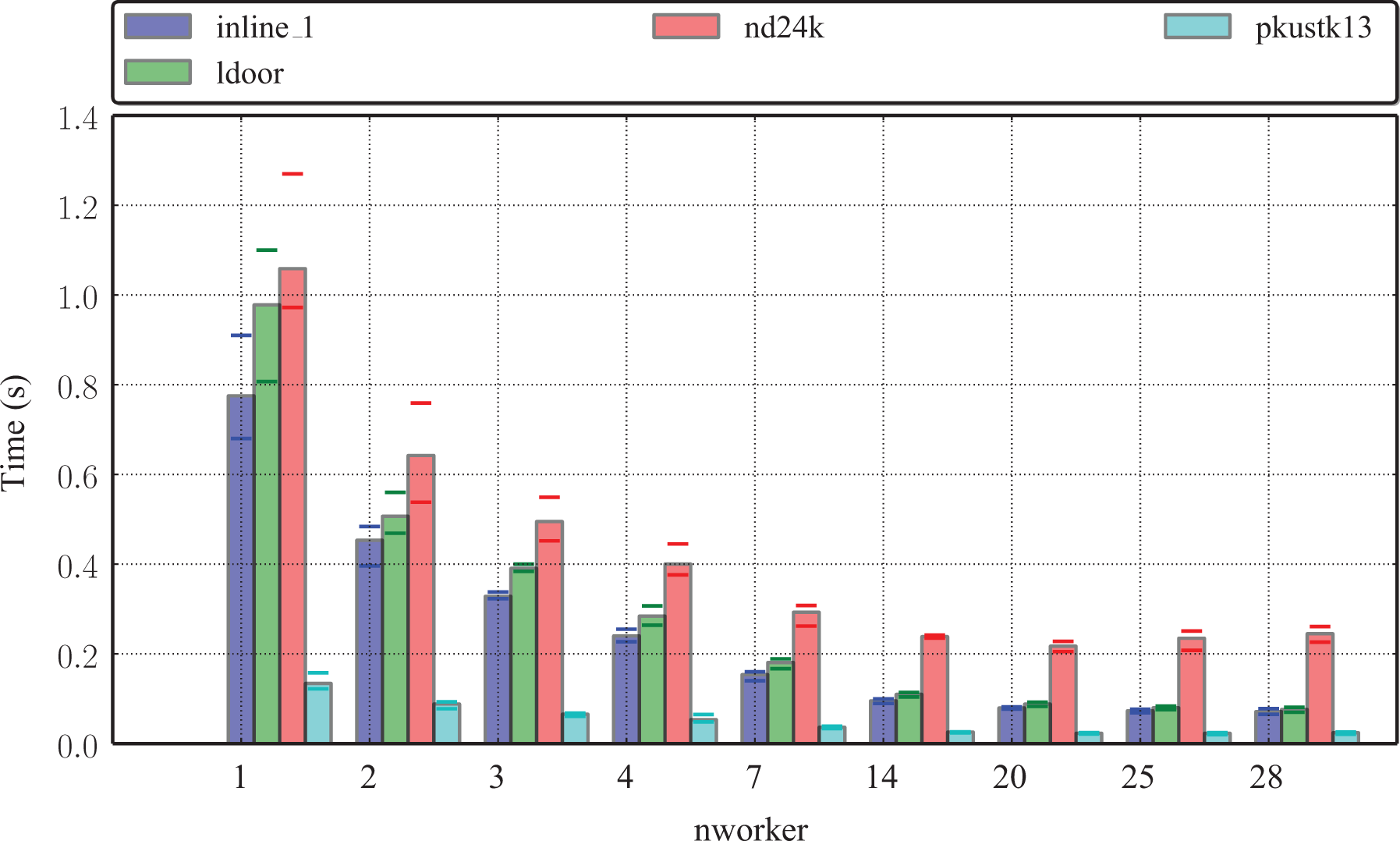
We perform the tests on a multicore machine which has two Intel Xeon E5-2695, v3 CPUs, that is 2 NUMA nodes composed of 14 cores each, with a total 128 GB of memory. Each core has a theoretical peak of 36.8 GFlop/s for a frequency of 2.3 GHz, so the peak of the multicore node is 1.03 TFlop/s in double precision. The code is compiled with GNU 6.2 and MKL 17.0.2 and linked to Metis 5.1.0 and SPRAL (https://github.com/ralna/spral/). In most cases, we display results on a representative subset of matrices. We have done preliminary tests to study the reproducibility of the execution times of the machine by solving equation (1) 10 times and increasing nworker. Figure 6 shows the range in the times for the solve phase on four of our test problems by horizontal bars. We note that this range can be noticeable when there are few workers, but this variability decreases markedly when nworker increases.

Figure 6.

Reproducibility of execution times.

We study the impact of pruning in Section 5.1, of synchronization tasks in Section 5.2 and of block size in Section 5.3. In Sections 5.4 and 5.5, we then compare the solve phase of SpLLT with Intel MKL PARDISO 17.0.2 (Schenk and Gärtner, 2002) and PaStiX (Hénon et al., 2002) by increasing nrhs in Section 5.4 and nworker in Section 5.5.

5.1. Impact of pruning on the performance

In this section, we illustrate the impact of using the tree pruning algorithm discussed in Section 4.3 on the solve times. For this, we performed the solve on a subset of the matrices given in Table 1 using one right-hand side and for a number of workers ranging between 1 and 28. Note that for this experiment, we selected the matrices which perform a high number of floating-point operations during the factorization. Our results, given in Table 2, include the solve times, with and without pruning, as well as the number of subtrees selected by the pruning algorithm when using 1, 2, 4, 14 and 28 workers.

Table 2.

The solve time (s) and number of subtrees when pruning is either enabled or disabled.

Matrices		#Worker
Matrices		1	2	4	14	28
boneS10	#Subtree	1	11	25	60	178
	No pruning	1.26	0.80	0.55	0.32	0.60
	With pruning	1.14	0.79	0.38	0.15	0.10
StocF-1465	#Subtree	29,105	29,108	29,115	29,177	29,189
	No pruning	3.03	2.54	1.46	0.82	1.51
	With pruning	2.83	2.41	1.27	0.66	0.75
Fault_639	#Subtree	1	5	18	43	88
	No pruning	4.02	2.23	1.07	0.43	0.55
	With pruning	2.48	2.05	0.99	0.40	0.33
Hook_1498	#Subtree	1	11	19	82	111
	No pruning	5.01	3.62	1.87	0.96	1.39
	With pruning	4.92	3.43	1.71	0.58	0.43
Emilia_923	#Subtree	1	6	21	67	99
	No pruning	5.10	2.85	1.59	0.65	0.83
	With pruning	4.66	2.77	1.49	0.61	0.47
Serena	#Subtree	1	5	11	37	110
	No pruning	6.42	4.88	2.72	1.12	1.35
	With pruning	6.13	4.56	2.41	0.96	0.76

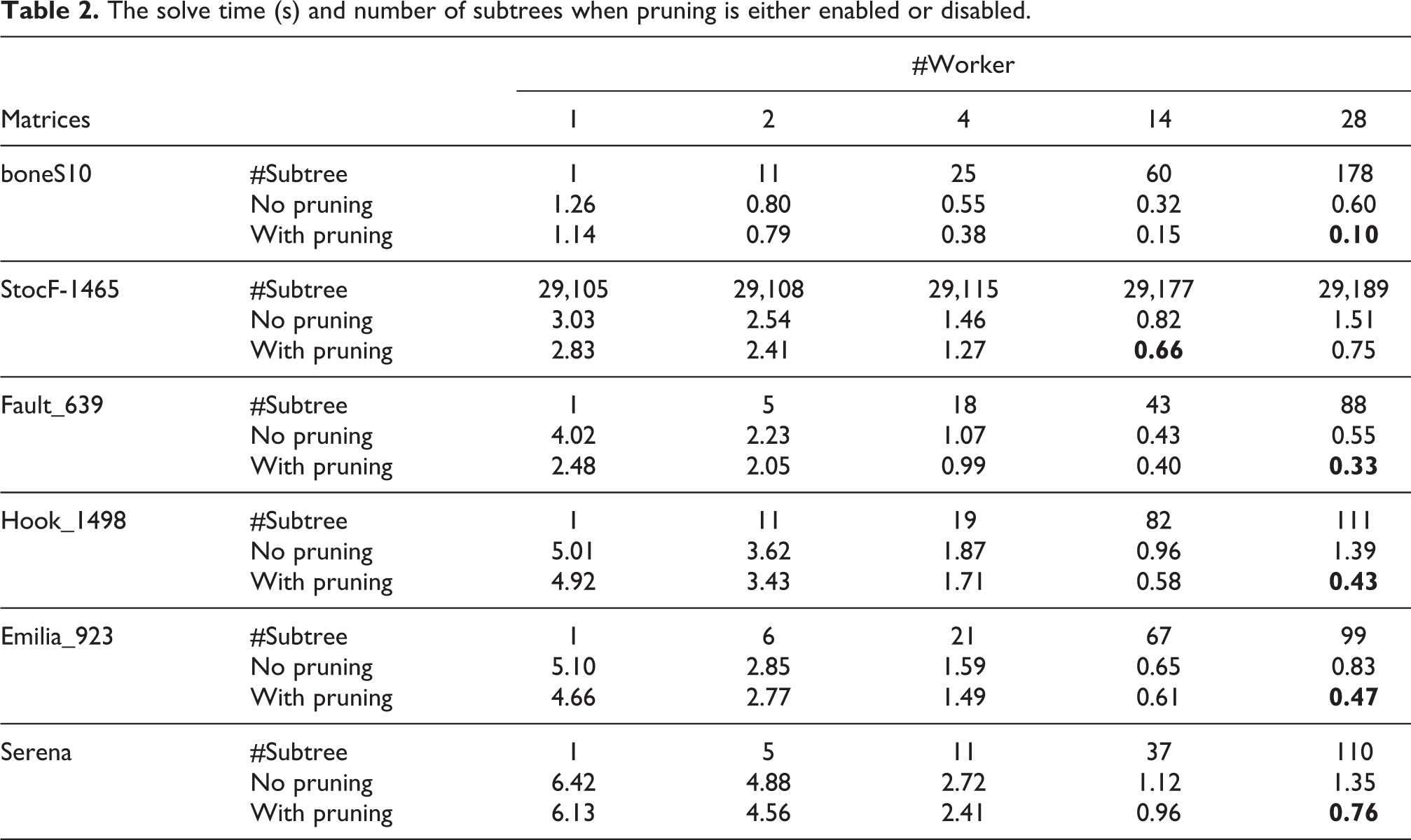
It should be noted that for all tested matrices, the best solve times are obtained when the tree pruning algorithm is enabled. Moreover, the impact of pruning is particularly high when nworker is large. For instance, enabling the tree pruning for boneS10 when using 2 workers is insignificant whereas the solve time is divided by a factor of 6 for this matrix when enabling tree pruning on 28 workers. Another notable effect of using tree pruning is that, although the solve times between 14 workers and 28 workers tend to increase without tree pruning, they keep decreasing if tree pruning is activated. This shows the benefits of using the pruning strategy to improve the scalability of our algorithm on a large number of resources.

As mentioned in Section 4.3, the tree pruning strategy improves the performance mainly for the following two reasons: firstly, it reduces the number of tasks in the DAG and more particularly small granularity tasks, and secondly, it increases kernel efficiency by improving the exploitation of data locality. This can be seen when looking at the data in the first column of Table 2. When using only one worker and disabling the pruning, all the tasks in the DAG are generated, submitted to the runtime system and processed by a single thread. On the other hand, when the pruning is enabled, the number of subtrees is equal to one which means that only one task, responsible for processing the whole tree, is generated. In this case, the cost for the task management is negligible and, as we can see in Table 2, the solve times are always reduced.

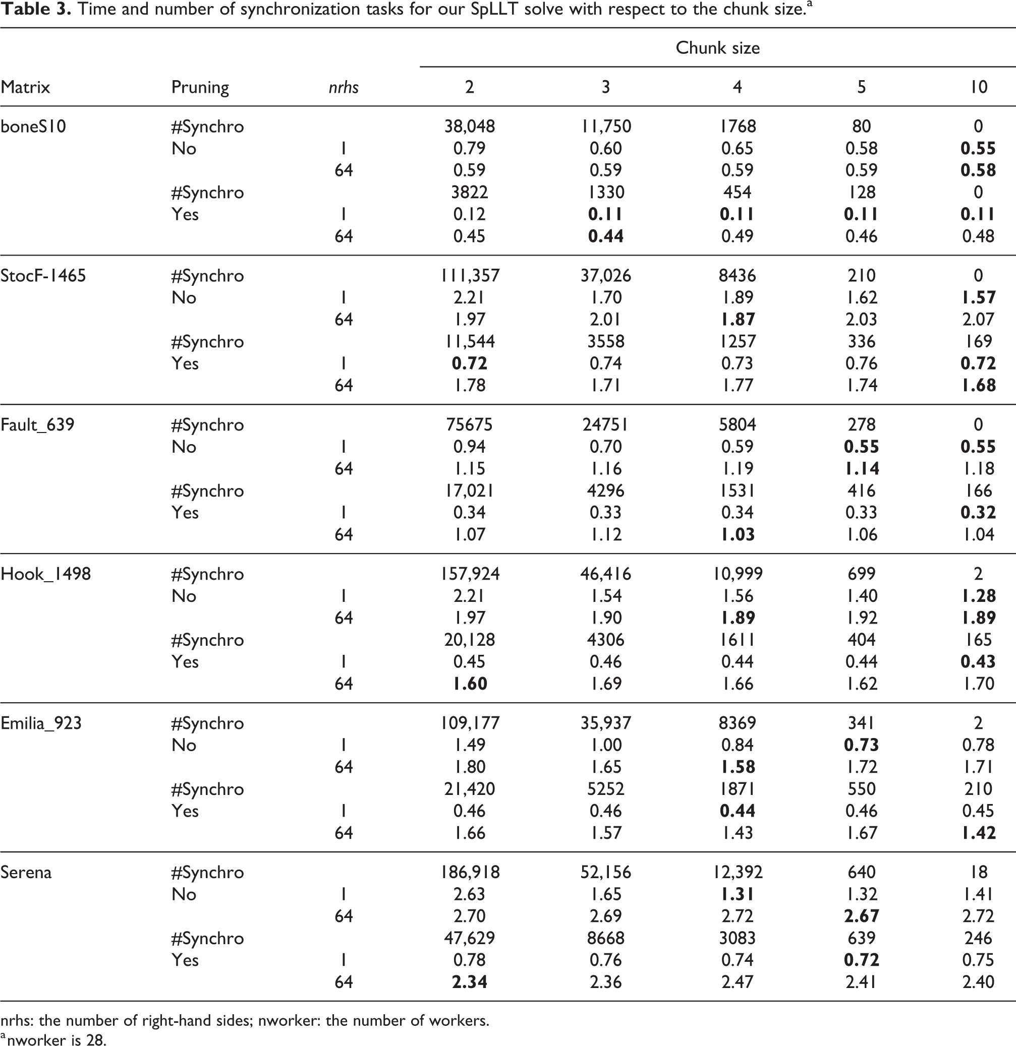
5.2. Impact of the number of synchronization tasks on the performance

As discussed in Section 4.2, tasks have a variable number of dependencies that we handle through a k-ary tree. In this section, we give details of the effect of the synchronization tasks on the solve time. We consider the case of 1 right-hand side and 64 right-hand sides. Table 3 presents the results on the same subset of matrices as in Table 2. We first focus on the case of one right-hand side where the pruning is disabled. We observe that the time to solve is the highest when c is equal to two. Moreover, the number of synchronization tasks is divided by at least a factor of 3 when increasing the chunk size from 2 to 3. After some point, the number of synchronization tasks is low enough that reducing it further does not noticeably improve the execution time. When pruning is used, we observe that the number of synchronization tasks is divided by at least a factor of 2 for a chunk size of 2. This means that the sensitivity of the times on the chunk size is much reduced when pruning is used. Likewise, when we solve for 64 right-hand sides, the extra work required means that the number of synchronization tasks has little impact on the time, with or without pruning. The arithmetic intensity in the kernels is much larger than the overhead of scheduling and executing synchronization tasks.

Table 3.

Time and number of synchronization tasks for our SpLLT solve with respect to the chunk size.^a

Matrix	Pruning	nrhs	Chunk size
Matrix	Pruning	nrhs	2	3	4	5	10
boneS10	#Synchro		38,048	11,750	1768	80	0
	No	1	0.79	0.60	0.65	0.58	0.55
	No	64	0.59	0.59	0.59	0.59	0.58
	#Synchro		3822	1330	454	128	0
	Yes	1	0.12	0.11	0.11	0.11	0.11
		64	0.45	0.44	0.49	0.46	0.48
StocF-1465	#Synchro		111,357	37,026	8436	210	0
	No	1	2.21	1.70	1.89	1.62	1.57
	No	64	1.97	2.01	1.87	2.03	2.07
	#Synchro		11,544	3558	1257	336	169
	Yes	1	0.72	0.74	0.73	0.76	0.72
		64	1.78	1.71	1.77	1.74	1.68
Fault_639	#Synchro		75675	24751	5804	278	0
	No	1	0.94	0.70	0.59	0.55	0.55
	No	64	1.15	1.16	1.19	1.14	1.18
	#Synchro		17,021	4296	1531	416	166
	Yes	1	0.34	0.33	0.34	0.33	0.32
		64	1.07	1.12	1.03	1.06	1.04
Hook_1498	#Synchro		157,924	46,416	10,999	699	2
	No	1	2.21	1.54	1.56	1.40	1.28
		64	1.97	1.90	1.89	1.92	1.89
	#Synchro		20,128	4306	1611	404	165
	Yes	1	0.45	0.46	0.44	0.44	0.43
		64	1.60	1.69	1.66	1.62	1.70
Emilia_923	#Synchro		109,177	35,937	8369	341	2
	No	1	1.49	1.00	0.84	0.73	0.78
	No	64	1.80	1.65	1.58	1.72	1.71
	#Synchro		21,420	5252	1871	550	210
	Yes	1	0.46	0.46	0.44	0.46	0.45
		64	1.66	1.57	1.43	1.67	1.42
Serena	#Synchro		186,918	52,156	12,392	640	18
	No	1	2.63	1.65	1.31	1.32	1.41
	No	64	2.70	2.69	2.72	2.67	2.72
	#Synchro		47,629	8668	3083	639	246
	Yes	1	0.78	0.76	0.74	0.72	0.75
		64	2.34	2.36	2.47	2.41	2.40

nrhs: the number of right-hand sides; nworker: the number of workers.

^a nworker is 28.

However, it is possible that for larger workloads than our test matrices, a small chunk size would penalize the performance because of a high number of synchronization tasks. For this reason, we use a chunk size of 10 in our solver that we consider to be large enough to avoid noticeable impact on the results on the tested matrices and potentially on bigger problems as well.

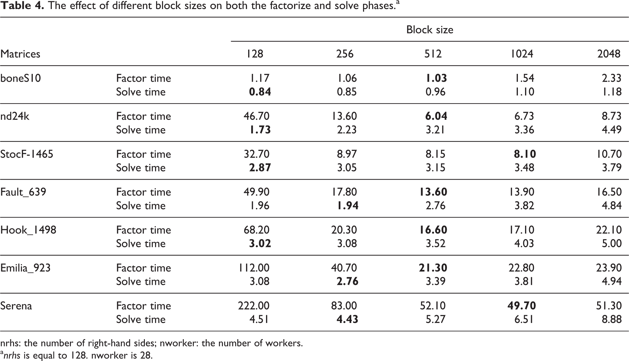
5.3. Impact of the block size on the performance

In this section, we study the impact of the block size on the time to solve the system and show our results in Table 4. We consider matrices that require a large number of flops during the factorization so that the block size should be greater than 256. We set nworker to 28 and nrhs to 128. For all these matrices, the optimal block size for the solve phase is lower than the optimal block size for the factorization. This leads us to conclude that we should use a different block size, depending on nrhs and the application. For example, in a code like preconditioned CG, the overall performance may depend on the time spent in applying the preconditioner. In that case, an efficient factorization is not as important as an optimal solve. We use a default block size of 256 in the following experiments to obtain a fair comparison with other solvers.

Table 4.

The effect of different block sizes on both the factorize and solve phases.^a

Matrices		Block size
Matrices		128	256	512	1024	2048
boneS10	Factor time	1.17	1.06	1.03	1.54	2.33
	Solve time	0.84	0.85	0.96	1.10	1.18
nd24k	Factor time	46.70	13.60	6.04	6.73	8.73
	Solve time	1.73	2.23	3.21	3.36	4.49
StocF-1465	Factor time	32.70	8.97	8.15	8.10	10.70
	Solve time	2.87	3.05	3.15	3.48	3.79
Fault_639	Factor time	49.90	17.80	13.60	13.90	16.50
	Solve time	1.96	1.94	2.76	3.82	4.84
Hook_1498	Factor time	68.20	20.30	16.60	17.10	22.10
	Solve time	3.02	3.08	3.52	4.03	5.00
Emilia_923	Factor time	112.00	40.70	21.30	22.80	23.90
	Solve time	3.08	2.76	3.39	3.81	4.94
Serena	Factor time	222.00	83.00	52.10	49.70	51.30
	Solve time	4.51	4.43	5.27	6.51	8.88

nrhs: the number of right-hand sides; nworker: the number of workers.

^a nrhs is equal to 128. nworker is 28.

5.4. Strong scaling on nrhs

In this section, we focus on the effect of nrhs on the time to solve the system. We fix nworker to 28 and the block size to 256, and we vary nrhs from 1 to 128 in powers of 2.

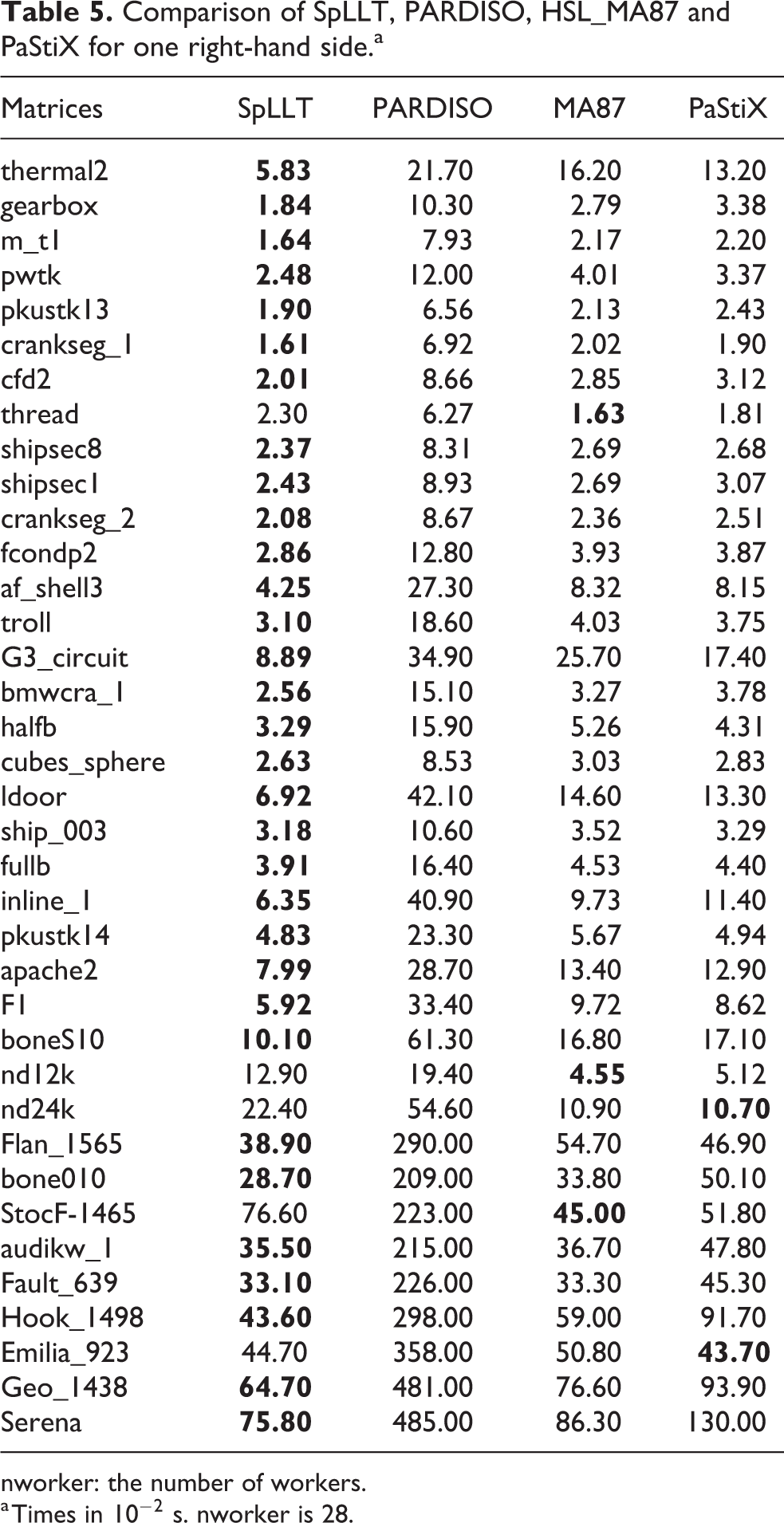
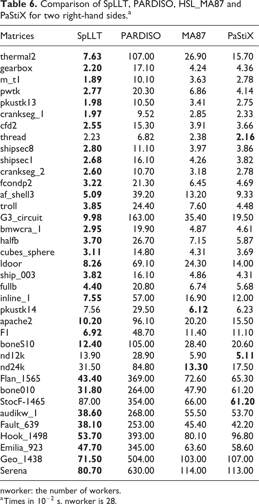
We first compare, in Tables 5 and 6, SpLLT with PARDISO, PaStiX and HSL_MA87 when solving for one or two right-hand sides. These results show that PARDISO is the slowest for all the matrices in Table 1. SpLLT is the fastest to solve the system, up to 8 times faster than PARDISO for one right-hand side and up to over a factor of 10 on two right-hand sides. There are only five problems in Table 1 for which SpLLT is not the fastest of all four codes for both one right-hand side and two right-hand sides. In two cases, the difference from the fastest code is marginal. The only matrices for which SpLLT is significantly slower are the two matrices nd12k and nd24k and the matrix StocF-1465. In the case of the first two, the assembly tree has long chains that are not combined by pruning so the runtime overhead for many small tasks causes the poor performance. If we force more node amalgamation in the analyse phase, the number of long chains decreases significantly, pruning is more effective, and we are much more competitive. The StocF-1465 matrix is very reducible with many 1 × 1 blocks. Again our pruning has little effect and we are penalized by the number of small tasks. We recommend that reducibility is respected in the solution process, and elimination techniques are only used on irreducible blocks. We see that on one of the matrices, Emilia_923, PaStiX is faster than SpLLT for one right-hand side (43.70 × 10⁻² s vs. 44.70 × 10⁻² s) and SpLLT is faster than PaStiX for two right-hand sides (47.70 × 10⁻² s vs. 58.6 × 10⁻² s). The solve time for SpLLT on two systems is always lower than solving one system twice.

Table 5.

Comparison of SpLLT, PARDISO, HSL_MA87 and PaStiX for one right-hand side.^a

Matrices	SpLLT	PARDISO	MA87	PaStiX
thermal2	5.83	21.70	16.20	13.20
gearbox	1.84	10.30	2.79	3.38
m_t1	1.64	7.93	2.17	2.20
pwtk	2.48	12.00	4.01	3.37
pkustk13	1.90	6.56	2.13	2.43
crankseg_1	1.61	6.92	2.02	1.90
cfd2	2.01	8.66	2.85	3.12
thread	2.30	6.27	1.63	1.81
shipsec8	2.37	8.31	2.69	2.68
shipsec1	2.43	8.93	2.69	3.07
crankseg_2	2.08	8.67	2.36	2.51
fcondp2	2.86	12.80	3.93	3.87
af_shell3	4.25	27.30	8.32	8.15
troll	3.10	18.60	4.03	3.75
G3_circuit	8.89	34.90	25.70	17.40
bmwcra_1	2.56	15.10	3.27	3.78
halfb	3.29	15.90	5.26	4.31
cubes_sphere	2.63	8.53	3.03	2.83
ldoor	6.92	42.10	14.60	13.30
ship_003	3.18	10.60	3.52	3.29
fullb	3.91	16.40	4.53	4.40
inline_1	6.35	40.90	9.73	11.40
pkustk14	4.83	23.30	5.67	4.94
apache2	7.99	28.70	13.40	12.90
F1	5.92	33.40	9.72	8.62
boneS10	10.10	61.30	16.80	17.10
nd12k	12.90	19.40	4.55	5.12
nd24k	22.40	54.60	10.90	10.70
Flan_1565	38.90	290.00	54.70	46.90
bone010	28.70	209.00	33.80	50.10
StocF-1465	76.60	223.00	45.00	51.80
audikw_1	35.50	215.00	36.70	47.80
Fault_639	33.10	226.00	33.30	45.30
Hook_1498	43.60	298.00	59.00	91.70
Emilia_923	44.70	358.00	50.80	43.70
Geo_1438	64.70	481.00	76.60	93.90
Serena	75.80	485.00	86.30	130.00

nworker: the number of workers.

^a Times in $10^{- 2}$ s. nworker is 28.

Table 6.

Comparison of SpLLT, PARDISO, HSL_MA87 and PaStiX for two right-hand sides.^a

Matrices	SpLLT	PARDISO	MA87	PaStiX
thermal2	7.63	107.00	26.90	15.70
gearbox	2.20	17.10	4.24	4.36
m_t1	1.89	10.10	3.63	2.78
pwtk	2.77	20.30	6.86	4.14
pkustk13	1.98	10.50	3.41	2.75
crankseg_1	1.97	9.52	2.85	2.33
cfd2	2.55	15.30	3.91	3.66
thread	2.23	6.82	2.38	2.16
shipsec8	2.80	11.10	3.97	3.86
shipsec1	2.68	16.10	4.26	3.82
crankseg_2	2.60	10.70	3.18	2.78
fcondp2	3.22	21.30	6.45	4.69
af_shell3	5.09	39.20	13.20	9.33
troll	3.85	24.40	7.60	4.48
G3_circuit	9.98	163.00	35.40	19.50
bmwcra_1	2.95	19.90	4.87	4.61
halfb	3.70	26.70	7.15	5.87
cubes_sphere	3.11	14.80	4.31	3.69
ldoor	8.26	69.10	24.30	14.00
ship_003	3.82	16.10	4.86	4.31
fullb	4.40	20.80	6.74	5.68
inline_1	7.55	57.00	16.90	12.00
pkustk14	7.56	29.50	6.12	6.23
apache2	10.20	96.10	20.20	15.50
F1	6.92	48.70	11.40	11.10
boneS10	12.40	105.00	28.40	20.60
nd12k	13.90	28.90	5.90	5.11
nd24k	31.50	84.80	13.30	17.50
Flan_1565	43.40	369.00	72.60	65.30
bone010	31.80	264.00	47.90	61.20
StocF-1465	87.00	354.00	66.00	61.20
audikw_1	38.60	268.00	55.50	53.70
Fault_639	38.10	253.00	45.40	42.20
Hook_1498	53.70	393.00	80.10	96.80
Emilia_923	47.70	345.00	63.60	58.60
Geo_1438	71.50	504.00	103.00	107.00
Serena	80.70	630.00	114.00	113.00

nworker: the number of workers.

^a Times in $10^{- 2}$ s. nworker is 28.

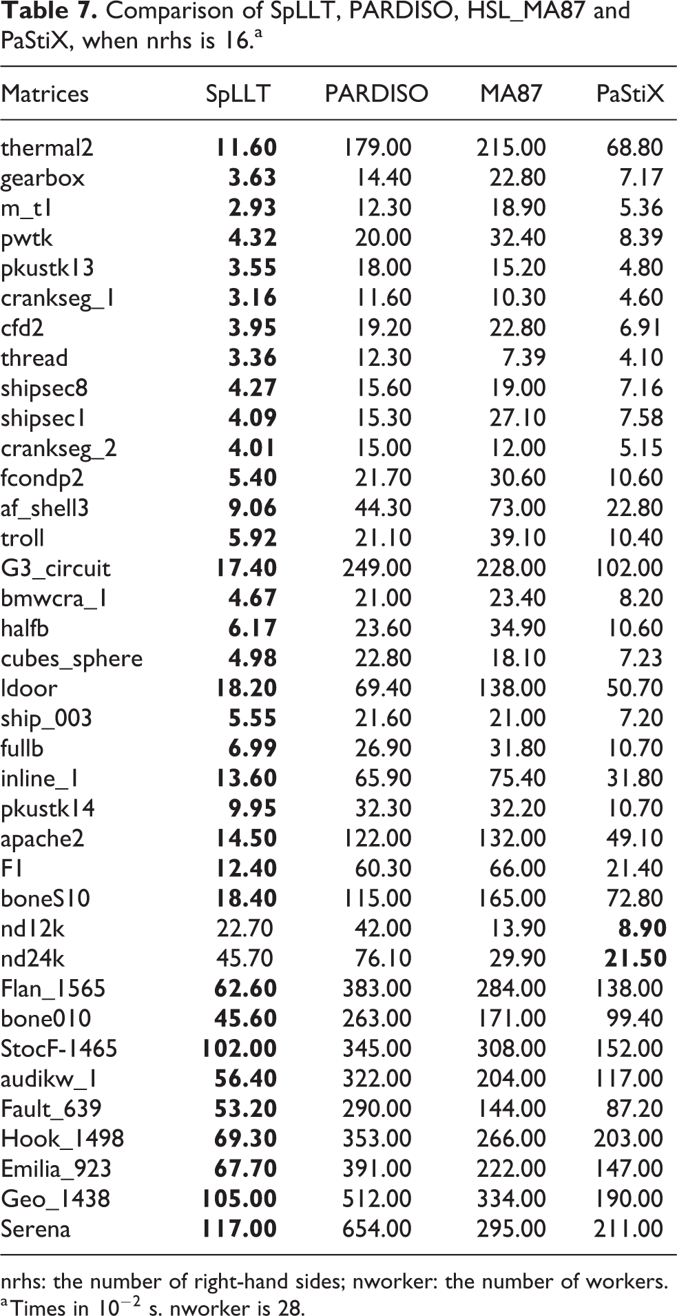
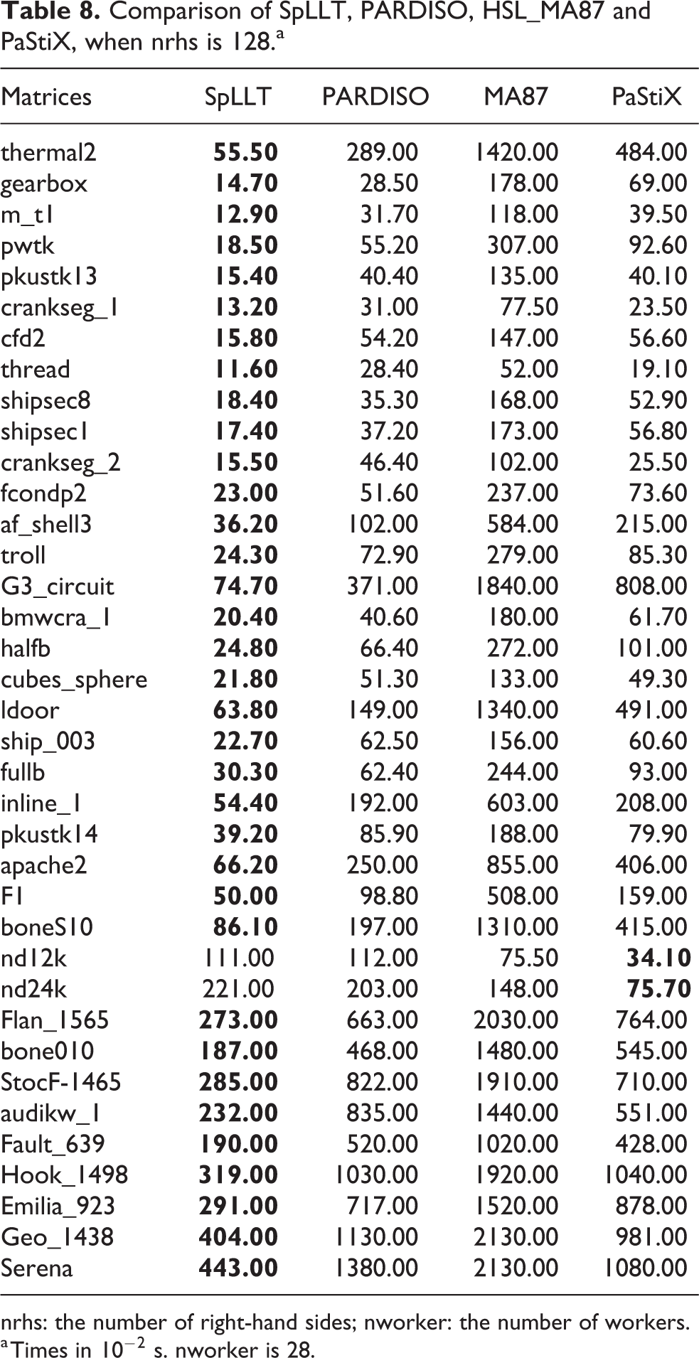
We investigate this for more right-hand sides. In Tables 7 and 8, we give the time for SpLLT, PARDISO, PaStiX and HSL_MA87, for all matrices of Table 1 when solving for 16 and 128 right-hand sides. When nrhs increases, PaStiX and HSL_MA87 become less competitive than SpLLT. We show the ratio of the time for solving several right-hand sides to the time to solve one right-hand side in Table 9. These results show that the power of level 3 BLAS means that there is often very little overhead for solving two right-hand sides over one and the extra cost when solving for 16 or 128 right-hand sides is remarkably low.

Table 7.

Comparison of SpLLT, PARDISO, HSL_MA87 and PaStiX, when nrhs is 16.^a

Matrices	SpLLT	PARDISO	MA87	PaStiX
thermal2	11.60	179.00	215.00	68.80
gearbox	3.63	14.40	22.80	7.17
m_t1	2.93	12.30	18.90	5.36
pwtk	4.32	20.00	32.40	8.39
pkustk13	3.55	18.00	15.20	4.80
crankseg_1	3.16	11.60	10.30	4.60
cfd2	3.95	19.20	22.80	6.91
thread	3.36	12.30	7.39	4.10
shipsec8	4.27	15.60	19.00	7.16
shipsec1	4.09	15.30	27.10	7.58
crankseg_2	4.01	15.00	12.00	5.15
fcondp2	5.40	21.70	30.60	10.60
af_shell3	9.06	44.30	73.00	22.80
troll	5.92	21.10	39.10	10.40
G3_circuit	17.40	249.00	228.00	102.00
bmwcra_1	4.67	21.00	23.40	8.20
halfb	6.17	23.60	34.90	10.60
cubes_sphere	4.98	22.80	18.10	7.23
ldoor	18.20	69.40	138.00	50.70
ship_003	5.55	21.60	21.00	7.20
fullb	6.99	26.90	31.80	10.70
inline_1	13.60	65.90	75.40	31.80
pkustk14	9.95	32.30	32.20	10.70
apache2	14.50	122.00	132.00	49.10
F1	12.40	60.30	66.00	21.40
boneS10	18.40	115.00	165.00	72.80
nd12k	22.70	42.00	13.90	8.90
nd24k	45.70	76.10	29.90	21.50
Flan_1565	62.60	383.00	284.00	138.00
bone010	45.60	263.00	171.00	99.40
StocF-1465	102.00	345.00	308.00	152.00
audikw_1	56.40	322.00	204.00	117.00
Fault_639	53.20	290.00	144.00	87.20
Hook_1498	69.30	353.00	266.00	203.00
Emilia_923	67.70	391.00	222.00	147.00
Geo_1438	105.00	512.00	334.00	190.00
Serena	117.00	654.00	295.00	211.00

nrhs: the number of right-hand sides; nworker: the number of workers.

^a Times in $10^{- 2}$ s. nworker is 28.

Table 8.

Comparison of SpLLT, PARDISO, HSL_MA87 and PaStiX, when nrhs is 128.^a

Matrices	SpLLT	PARDISO	MA87	PaStiX
thermal2	55.50	289.00	1420.00	484.00
gearbox	14.70	28.50	178.00	69.00
m_t1	12.90	31.70	118.00	39.50
pwtk	18.50	55.20	307.00	92.60
pkustk13	15.40	40.40	135.00	40.10
crankseg_1	13.20	31.00	77.50	23.50
cfd2	15.80	54.20	147.00	56.60
thread	11.60	28.40	52.00	19.10
shipsec8	18.40	35.30	168.00	52.90
shipsec1	17.40	37.20	173.00	56.80
crankseg_2	15.50	46.40	102.00	25.50
fcondp2	23.00	51.60	237.00	73.60
af_shell3	36.20	102.00	584.00	215.00
troll	24.30	72.90	279.00	85.30
G3_circuit	74.70	371.00	1840.00	808.00
bmwcra_1	20.40	40.60	180.00	61.70
halfb	24.80	66.40	272.00	101.00
cubes_sphere	21.80	51.30	133.00	49.30
ldoor	63.80	149.00	1340.00	491.00
ship_003	22.70	62.50	156.00	60.60
fullb	30.30	62.40	244.00	93.00
inline_1	54.40	192.00	603.00	208.00
pkustk14	39.20	85.90	188.00	79.90
apache2	66.20	250.00	855.00	406.00
F1	50.00	98.80	508.00	159.00
boneS10	86.10	197.00	1310.00	415.00
nd12k	111.00	112.00	75.50	34.10
nd24k	221.00	203.00	148.00	75.70
Flan_1565	273.00	663.00	2030.00	764.00
bone010	187.00	468.00	1480.00	545.00
StocF-1465	285.00	822.00	1910.00	710.00
audikw_1	232.00	835.00	1440.00	551.00
Fault_639	190.00	520.00	1020.00	428.00
Hook_1498	319.00	1030.00	1920.00	1040.00
Emilia_923	291.00	717.00	1520.00	878.00
Geo_1438	404.00	1130.00	2130.00	981.00
Serena	443.00	1380.00	2130.00	1080.00

nrhs: the number of right-hand sides; nworker: the number of workers.

^a Times in $10^{- 2}$ s. nworker is 28.

Table 9.

Ratio of time _nrhs /time_1rhs.

Matrix	Time 1rhs ( $10^{- 2}$ s)	$T_{2} / T_{1}$	$T_{16} / T_{1}$	$T_{128} / T_{1}$
boneS10	10.10	1.23	1.82	8.52
nd12k	12.90	1.08	1.76	8.60
nd24k	22.40	1.41	2.04	9.87
Flan_1565	38.90	1.12	1.61	7.02
bone010	28.70	1.11	1.59	6.52
StocF-1465	76.60	1.14	1.33	3.72
audikw_1	35.50	1.09	1.59	6.54
Fault_639	33.10	1.15	1.61	5.74
Hook_1498	43.60	1.23	1.59	7.32
Emilia_923	44.70	1.07	1.51	6.51
Geo_1438	64.70	1.11	1.62	6.24
Serena	75.80	1.06	1.54	5.84

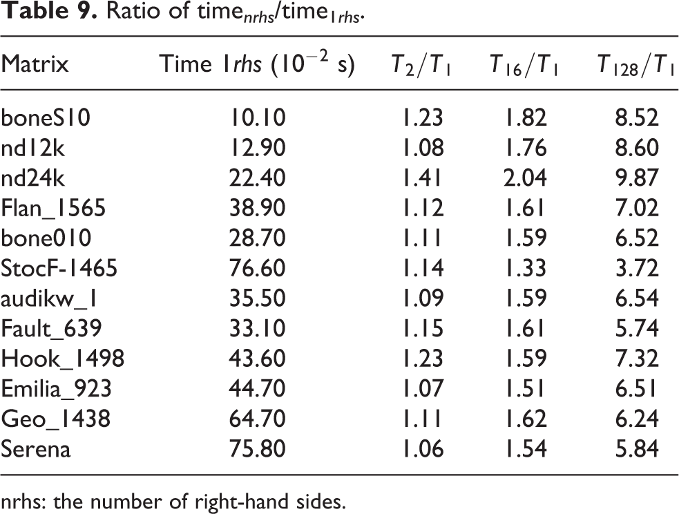
nrhs: the number of right-hand sides.

Since HSL_MA87 does not scale with nrhs, in the following, we compare the time to solve for SpLLT with PARDISO and PaStiX, and we display the ratio of times in Figure 7.

Figure 7.

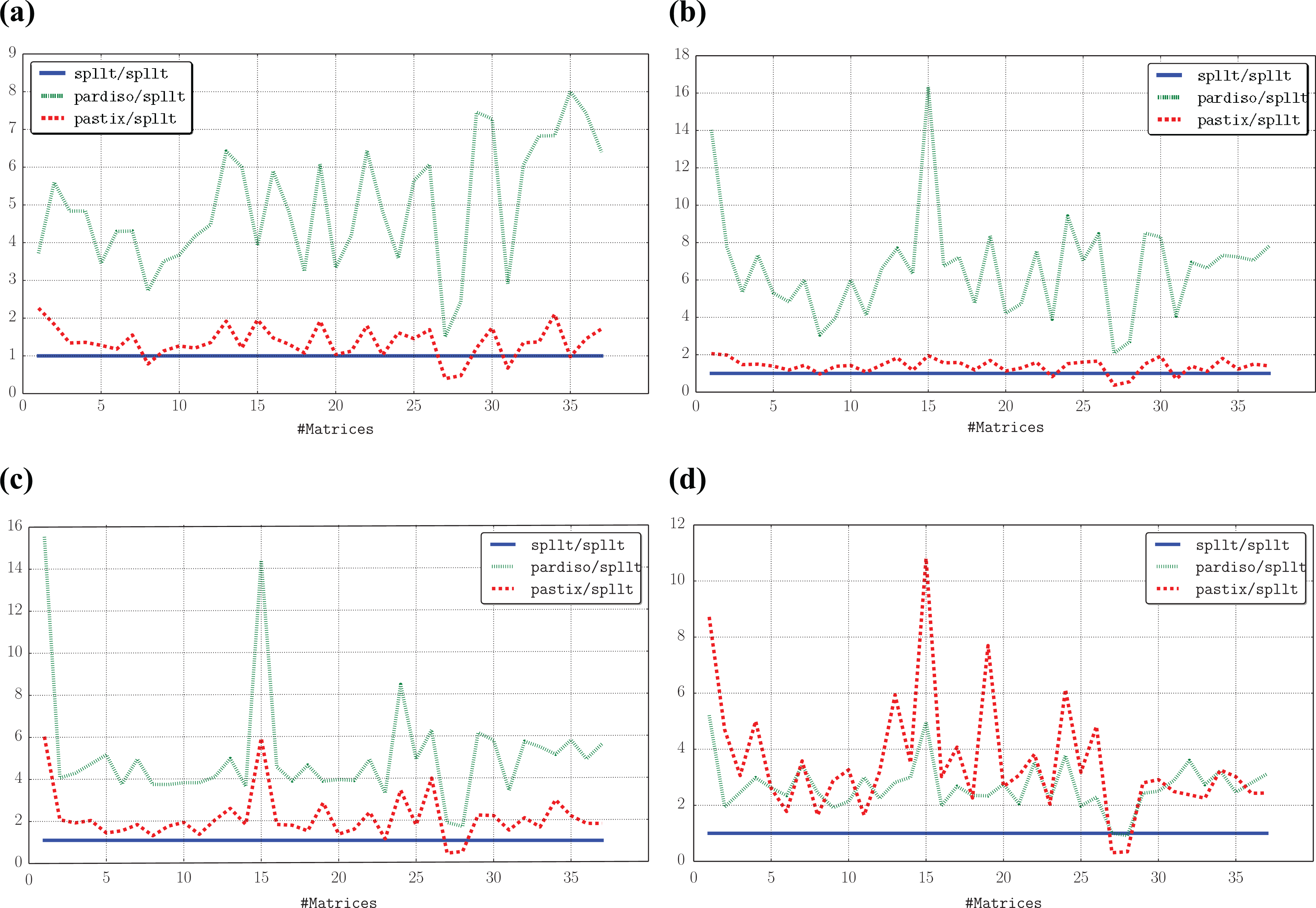
Comparison of the times to solve the system with multiple right-hand sides using PARDISO and PaStiX, relative to SpLLT. nworker is set to 28, and nrhs is equal to (a) 1, (b) 2, (c) 16 and (d) 128. nrhs: the number of right-hand sides; nworker: the number of workers.

Figure 8 presents two representative problems that illustrate the behaviour of each solver. For all nrhs, SpLLT is the fastest solver sometimes by a considerable amount. PaStiX scales much worse than SpLLT as nrhs increases. The scalability of PARDISO can vary considerably (see Serena). Since the source code for PARDISO is not distributed, we do not know why this is the case. We have similarly erratic scalability for several other matrices in our test set. In Figure 8(a), SpLLT is eight times faster than PARDISO for two right-hand sides, and these two curves increase almost similarly when nrhs increases. On the other hand, the time to solve using PaStiX is close to SpLLT for 2 right-hand sides but is 5 times slower on 128 right-hand sides. In general, SpLLT scales better than the other codes.

Figure 8.

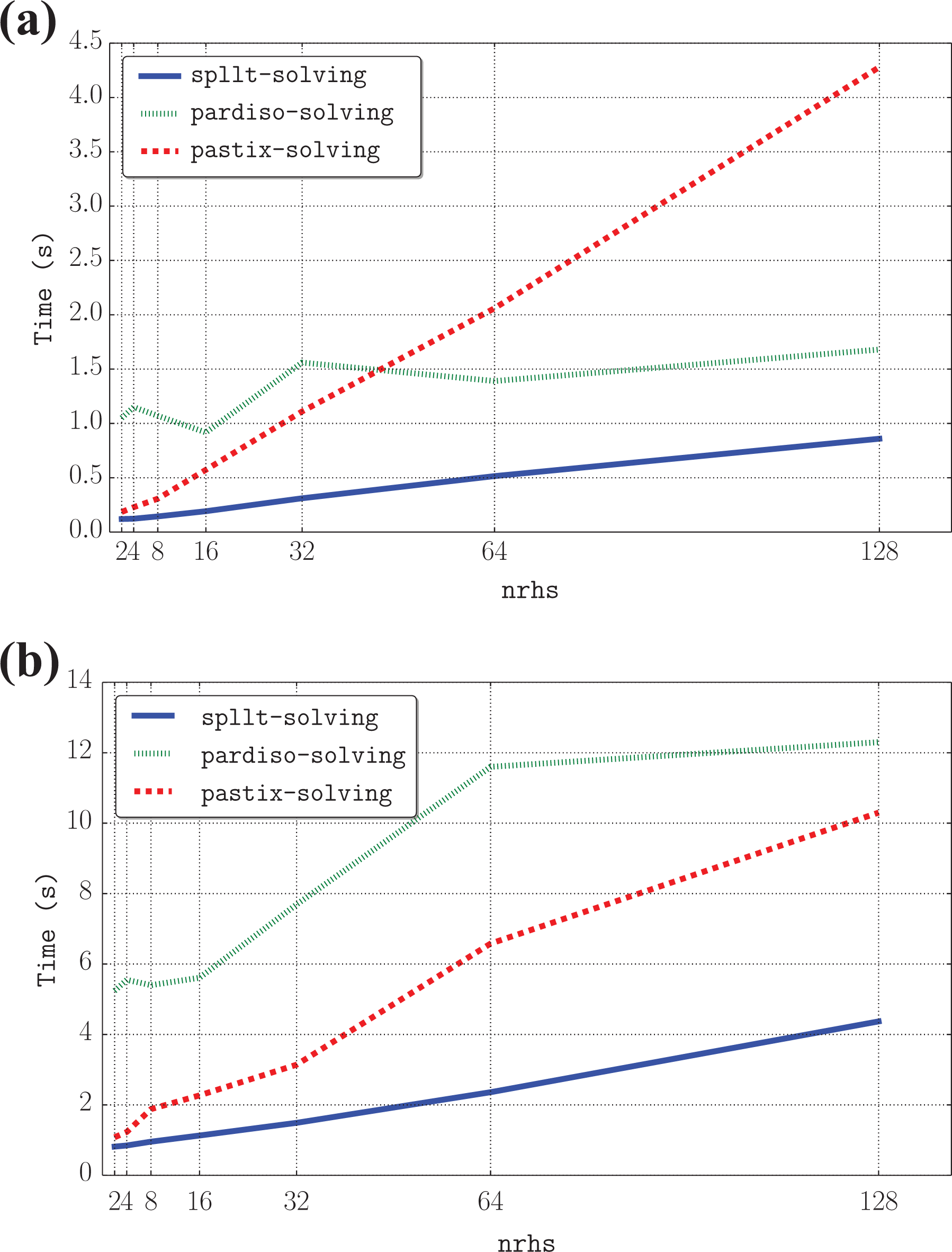
Comparison of the time to solve the system with multiple right-hand sides using SpLLT, PARDISO and PaStiX. nworker is set to 28, and nrhs increases from 2 to 128 in powers of 2. (a) boneS10 and (b) Serena. nrhs: the number of right-hand sides; nworker: the number of workers.

5.5. Strong scaling on nworker

In this section, we study the impact of nworker on the time to solve a system with 1 right-hand side and 64 right-hand sides. nworker increases from 1 to 28, and the block size is 256. We first consider one right-hand side and present some results in Figure 9. We use the same two matrices as in Figure 8. The experiments show that for a small number of workers, the time to solve using SpLLT is greater than both other solvers. When nworker increases, the solid curve that represents SpLLT becomes closer to the other curves. For 28 workers, SpLLT is the fastest solver.

Figure 9.

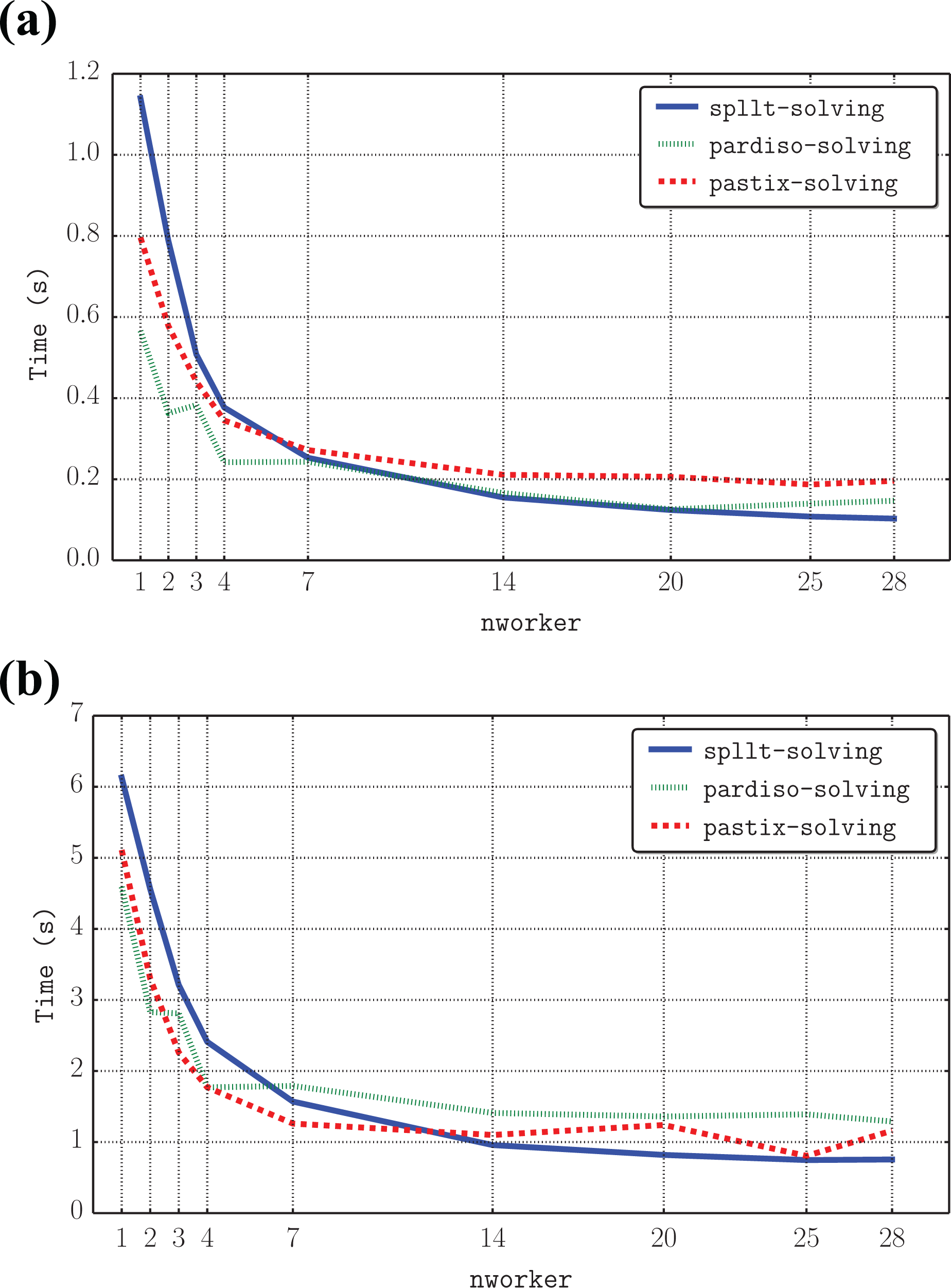
Comparison of the time to solve the system with one right-hand side for SpLLT, PARDISO and PaStiX. (a) boneS10 and (b) Serena.

Figure 10 shows the impact of increasing nworker when there are 64 right-hand sides. SpLLT is more competitive than for a small nrhs. In fact, SpLLT outperforms PARDISO for all numbers of workers and is faster than PaStiX when nworker increases. For more than nine workers, these two representative problems show that SpLLT is clearly the fastest solver.

Figure 10.

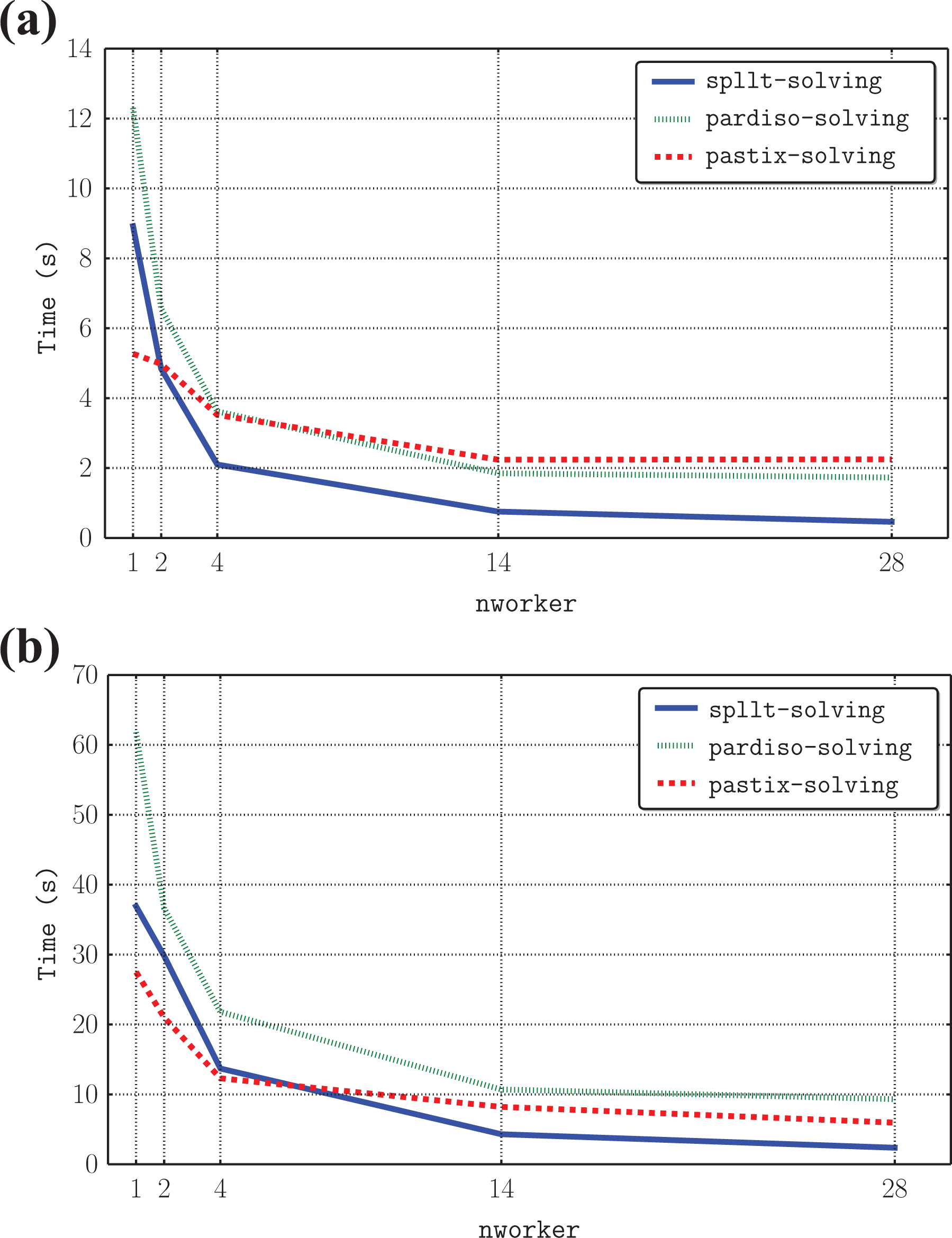
Comparison of the time to solve the system with 64 right-hand sides for SpLLT, PARDISO and PaStiX. (a) boneS10 and (b) Serena.

5.6. Application case: Enlarged CG solver

In this section, we present some results obtained with the enlarged CG solver (ECG) (Grigori and Tissot, 2017). Our runs in this section are on a different machine to our earlier results. We use the Kebnekaise system at Umeå in Sweden (https://www.hpc2n.umu.se/resources/hardware/kebnekaise). Each compute node contains 28 Intel Xeon E5-2690v4 cores organized into 2 NUMA islands with 14 cores in each. The nodes are connected with an FDR Infiniband Network. The total amount of RAM per compute node is 128 GB. ECG and SpLLT are compiled with Intel 18.0.1 and linked to Metis 5.1.0.

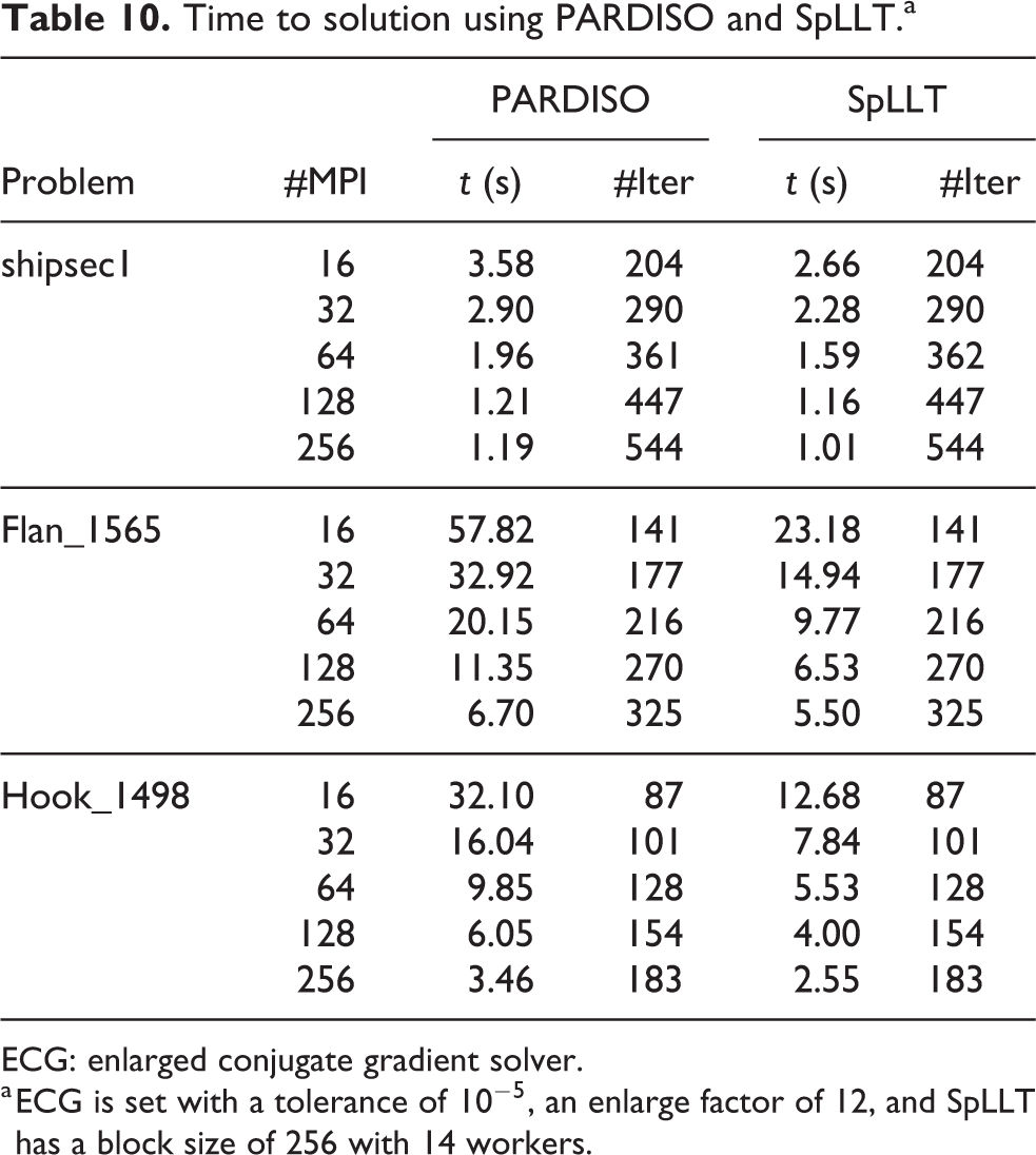
The ECG solver is a preconditioned CG solver that augments the number of working vectors to reduce the number of iterations as well as to obtain better parallelism and to reduce the amount of communication. ECG uses a block Jacobi preconditioner. Although each diagonal block is factorized only once, the solve of each associated local system is performed at each iteration of ECG. Table 10 presents the time to solve the global system with ECG using PARDISO or SpLLT on a subset of matrices from Table 1. We show results from 16 MPI processes to 256 MPI processes. We see little difference in solution times for the shipsec1 problem but, on the two other problems that are 10 times larger, we observe that replacing the PARDISO Solver with the SpLLT solver leads to a speed-up over a factor of 2. In all cases, solving the system with 16 MPI processes using SpLLT is faster than using PARDISO with 32 MPI processes.

Table 10.

Time to solution using PARDISO and SpLLT.^a

Problem	#MPI	PARDISO		SpLLT
Problem	#MPI	t (s)	#Iter	t (s)	#Iter
shipsec1	16	3.58	204	2.66	204
	32	2.90	290	2.28	290
	64	1.96	361	1.59	362
	128	1.21	447	1.16	447
	256	1.19	544	1.01	544
Flan_1565	16	57.82	141	23.18	141
	32	32.92	177	14.94	177
	64	20.15	216	9.77	216
	128	11.35	270	6.53	270
	256	6.70	325	5.50	325
Hook_1498	16	32.10	87	12.68	87
	32	16.04	101	7.84	101
	64	9.85	128	5.53	128
	128	6.05	154	4.00	154
	256	3.46	183	2.55	183

ECG: enlarged conjugate gradient solver.

^a ECG is set with a tolerance of $10^{- 5}$ , an enlarge factor of 12, and SpLLT has a block size of 256 with 14 workers.

6. Conclusions

We have designed, implemented and tested new routines for the forward and backward substitution steps in the parallel solution of sparse positive definite systems using a Cholesky factorization. We have given details of how our design exploits parallelism while keeping data movement low. We have developed a code that we have tested on a multicore node and have targeted and achieved good scalability both with respect to the number of cores and to nrhs. We have compared our code to other state-of-the-art codes and shown that it is usually far superior sometimes outperforming the other codes by a factor of over 10. We have shown that our code is strongly scalable both for cores and right-hand sides.

Finally, we have tested our code within a real application and shown big gains over the previous version that used another solver. We are continuing our work with the authors of ECG at Inria and have seen even bigger gains on markedly larger problems than those used in this article. For example, on a matrix from a diffusion problem of order nearly 5 million with over 34 million entries, we reduce the solution time by a factor of nearly 3 on 16 MPI processes and by a factor of nearly 2 on 256 processes.

Footnotes

Acknowledgements

The authors would like to thank Tyrone Rees of RAL for his comments on an early draft of this article and the High Performance Computing Center North (HPC2N) at Umeå University for providing computational resources and valuable support for the work in Section 5.6.

Declaration of conflicting interests

The author(s) declared no potential conflicts of interest with respect to the research, authorship, and/or publication of this article.

Funding

The author(s) disclosed receipt of the following financial support for the research, authorship, and/or publication of this article: This work was supported by the NLAFET Project funded by the European Union’s Horizon 2020 Research and Innovation Programme under Grant Agreement 671633.

ORCID iD

Sébastien Cayrols

References

Amestoy

Davis

Duff

(1996) An approximate minimum degree ordering algorithm. SIAM Journal on Matrix Analysis and Applications 17(4): 886–905. DOI: 10.1137/S0895479894278952.

Augonnet

Thibault

Namyst

, et al. (2011) StarPU: a unified platform for task scheduling on heterogeneous multicore architectures. Concurrency and Computation: Practice and Experience, Special Issue: Euro-Par 2009 23: 187–198. DOI:10.1002/cpe.1631. Available at: http://hal.inria.fr/inria-00550877 (accessed 12 November 2019).

Blackford

Demmel

Dongarra

, et al. (2002) An updated set of basic linear algebra subprograms (BLAS). ACM Transactions on Mathematical Software 28(2): 135–151.

Bosilca

Bouteiller

Danalis

, et al. (2013) PaRSEC: exploiting heterogeneity to enhance scalability. Computing in Science and Engineering 15(6): 36–45. DOI: 10.1109/MCSE.2013.98.

Buttari

(2012) Fine granularity sparse QR factorization for multicore based systems. In: Jónasson

(ed.) Applied Parallel and Scientific Computing. Berlin, Heidelberg: Springer Berlin Heidelberg, pp. 226–236. ISBN 978-3-642-28145-7.

Davis

(2011) The University of Florida sparse matrix collection. ACM Transactions on Mathematical Software 38(1): 1:1–1:25. DOI: 10.1145/2049662.2049663.

Duff

Lopez

(2018) Experiments with sparse Cholesky using a parametrized task graph implementation. In: Wyrzykowski

Dongarra

Deelman

Karczewski

(eds) Parallel Processing and Applied Mathematics. Cham: Springer International Publishing, pp. 197–206. ISBN 978-3-319-78024-5.

Duff

Erisman

Reid

(2017) Direct Methods for Sparse Matrices, 2nd ed. Oxford, UK: Oxford University Press. ISBN 987-0-19-850838-0 (hardcover).

Duff

Hogg

Lopez

(2018) Experiments with sparse Cholesky using a sequential task-flow implementation. Numerical Algebra, Control and Optimization 8: 235–258.

10.

Grigori

Tissot

(2017) Reducing the Communication and Computational Costs of Enlarged Krylov Subspaces Conjugate Gradient: Research Report RR-9023. Paris: Inria. Available at: https://hal.inria.fr/hal-01451199v2/document (accessed 12 November 2019).

11.

Hénon

Ramet

Roman

(2002) PaStiX: a high-performance parallel direct solver for sparse symmetric definite systems. Parallel Computing 28(2): 301–321. Available at: https://hal.inria.fr/inria-00346017 (accessed 12 November 2019).

12.

Hogg

Reid

Scott

(2010) Design of a multicore sparse Cholesky factorization using DAGs. SIAM Journal on Scientific Computing 32(6): 3627–3649. DOI: 10.1137/090757216.

13.

Karypis

Kumar

(1998) Multilevel k-way partitioning scheme for irregular graphs. Journal of Parallel and Distributed Computing 48: 96–129.

14.

Schenk

Gärtner

(2002) Two-level dynamic scheduling in PARDISO: improved scalability on shared memory multiprocessing systems. Parallel Computing 28(2): 187–197.