
Abstract
A nonlinear domain decomposition (DD) solver is considered with respect to improved energy efficiency. In this method, nonlinear problems are solved using Newton’s method on the subdomains in parallel and in asynchronous iterations. The method is compared to the more standard Newton-Krylov approach, where a linear domain decomposition solver is applied to the overall nonlinear problem after linearization using Newton’s method. It is found that in the nonlinear domain decomposition method, making use of the asynchronicity, some processor cores can be set to sleep to save energy and to allow better use of the power and thermal budget. Energy savings on average for each socket up to 77% (due to the RAPL hardware counters) are observed compared to the more traditional Newton-Krylov approach, which is synchronous by design, using up to 5120 Intel Broadwell (Xeon E5-2630v4) cores. The total time to solution is not affected. On the contrary, remaining cores of the same processor may be able to go to turbo mode, thus reducing the total time to solution slightly. Last, we consider the same strategy for the ASPIN (Additive Schwarz Preconditioned Inexact Newton) nonlinear domain decomposition method and observe a similar potential to save energy.
Keywords
1. Introduction
In recent years, many nonlinear domain decomposition approaches have been introduced and their superiority over the classical combination of a nonlinear solver, e.g. Newton’s method, with a linear domain decomposition approach has been shown for many model problems (Cai and Keyes, 2002; Cai et al., 2002a, 2002b; Dolean et al., 2016; Groß, 2009; Groß and Krause, 2011; Klawonn et al., 2014, 2015, 2016, 2017, 2018; Liu and Keyes, 2015; Liu et al., 2018; Marcinkowski and Cai, 2005; Negrello et al., 2018). Nonlinear domain decomposition methods are solution approaches for nonlinear problems and apply the concepts and ideas of linear domain decomposition methods as, e.g. Overlapping Schwarz (Cai and Keyes, 2002; Cai et al., 2002a, 2002b; Dolean et al., 2016; Groß, 2009; Groß and Krause, 2011; Liu and Keyes, 2015; Liu et al., 2018; Marcinkowski and Cai, 2005), FETI (Finite Element Tearing and Interconnecting) (Negrello et al., 2018), FETI-DP (Finite Element Tearing and Interconnecting—Dual-Primal) (Klawonn et al., 2014, 2015, 2017), and BDDC (Balancing Domain Decomposition by Constraints) (Klawonn et al., 2014, 2017, 2018) directly to a nonlinear problem before a nonlinear solver is applied. Although all these methods behave quite differently in their linear as well as nonlinear variants, they have some common features and properties. We will show that one of these properties makes nonlinear domain decomposition methods typically more energy efficient compared with their linear relatives embedded in some nonlinear solver. This effect is not only caused by a shorter runtime but also the power consumption is typically lower during most of the computation. In this paper, we will show and explain this effect in detail for the example of nonlinear FETI-DP methods. First we will provide a more general description of the concept and show that it is also applicable to other methods as, e.g. ASPIN (Additive Schwarz Preconditioned Inexact Newton) (Cai and Keyes, 2002).
Given is a discrete nonlinear problem

which has been obtained by a discretization of a nonlinear partial differential equation. In contrast to classical approaches, e.g. Newton-Krylov-DD (Domain Decomposition) methods, where eq. (1) is linearized by Newton’s method and the tangential system is solved iteratively using a domain decomposition approach, the discrete nonlinear function eq. (1) is replaced by an alternative formulation

Here,
Of course, it has to be guaranteed that eq. (1) and eq. (2) have the same solution. Then, instead of eq. (1), eq. (2) is solved by a nonlinear solver. If

or as a a nonlinear left-preconditioning approach

Examples for the latter case are ASPIN (Cai and Keyes, 2002) and RASPEN (Dolean et al., 2016), while Nonlinear-FETI-DP and Nonlinear-BDDC can be interpreted as nonlinearly right preconditioned methods; see Klawonn et al. (2017). To be efficient, applications of the preconditioners M and G should be cheap compared with an application of A. Both should put the initial value near to the solution and to obtain the correct solution, one has to ensure that
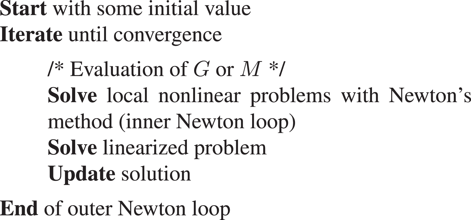
Sketch of a nonlinear domain decomposition method using Newton’s method.
However, some of the local nonlinear problems in G or M can converge fast or even in a single step (nearly linear behavior), while others may take many Newton steps to converge. Under the assumption that each computational core solves exactly one local nonlinear problem, problem dependent load imbalances can thus arise. This can be tolerated as long as the time to solution is faster than using classical approaches with proper load balance, but is nonetheless a topic of current research. Removing the load imbalance completely without loosing convergence properties is difficult since a redistribution of the work, e.g. by resizing subdomains changes the nonlinear problem
In this paper, we investigate a different approach and decide to set cores to sleep (test-and-sleep), when they have finished solving their local nonlinear problem until all other cores catch up. This can save energy compared to classical approaches and is feasible because the desynchronization of the local Newton iterations in nonlinear DD methods results in potential sleep times at the order of seconds; see Section 4. To demonstrate this effect, we compare the classical Newton-Krylov-FETI-DP approach with Nonlinear-FETI-DP-3 with respect to scalability, runtime, load balancing, energy consumption, and power efficiency. Let us remark here that Nonlinear-FETI-DP-3 is a good testing prototype, since completely decoupled local nonlinear problems are solved in each outer Newton step. Nonetheless, all introduced concepts can be carried over to different nonlinear DD methods and, even more generally, to many other applications with a severe load imbalance. Note that, here, we do not propose test-and-sleep as a universal method to save energy. It is rather used to show the energy saving potential of new algorithms, i.e. nonlinear domain decomposition.
The remainder of the paper is organized as follows. In Section 2 in order to provide a self-contained paper, we give a detailed description of Newton-Krylov-FETI-DP and Nonlinear-FETI-DP-3 with a focus on the local solves and the load imbalance in the latter one. We describe the investigated model problems in Section 3 and our approach to save energy as well as corresponding measurements in Section 4. Finally, in Section 5, we provide a model to interprete the measurements resulting from Section 4.
2. An introduction to nonlinear FETI-DP methods
In this section, we briefly introduce the nonlinear FETI-DP (Finite Element Tearing and Interconnecting—Dual Primal) framework (see Klawonn et al., 2014, 2017 for a detailed description) and derive Nonlinear-FETI-DP-3, the variant we use in this paper to represent nonlinear domain decomposition methods. As already mentioned above, instead of solving eq. (1) directly by applying Newton’s method, in nonlinear FETI-DP methods eq. (1) is replaced by the equivalent formulation

which is then solved by a Newton-Krylov approach. Here,
Let us first summarize linear FETI-DP and introduce the classical Newton-Krylov-FETI-DP method in subsection 2.1 before we proceed to describe the nonlinear variant in the following subsections.
2.1. Newton-Krylov-FETI-DP
In general, we assume that eq. (1) is obtained by a finite element discretization of a partial differential equation defined on a computational domain

where

Here,
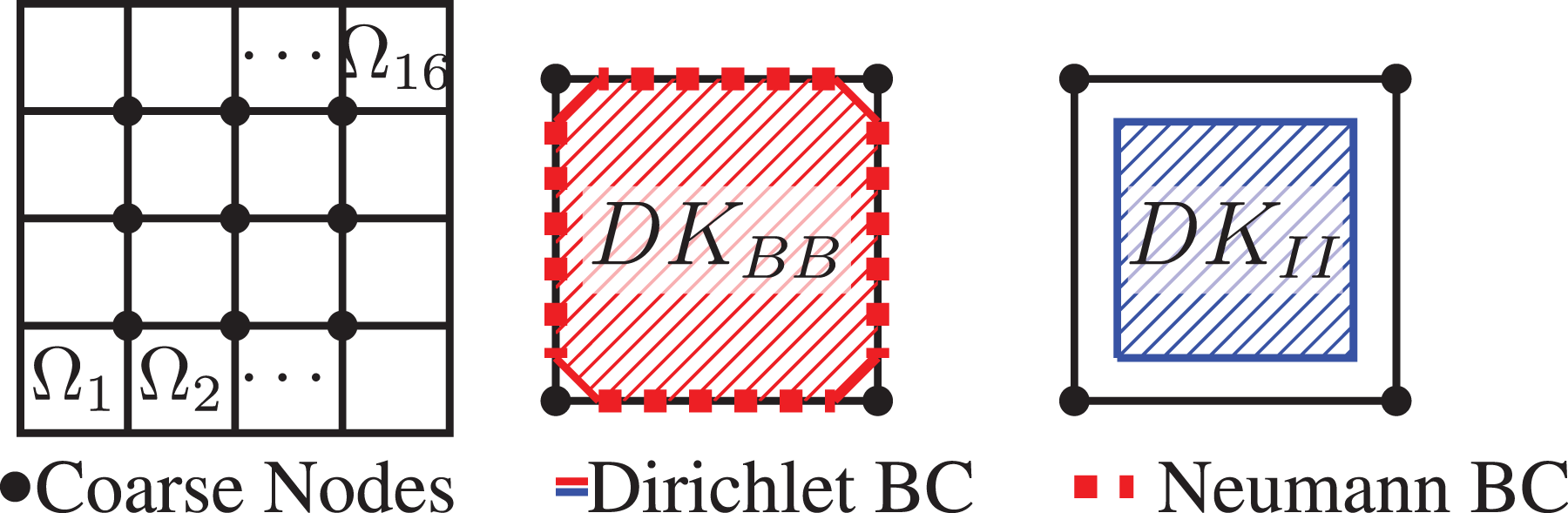
Let us briefly describe linear FETI-DP and introduce some necessary notation. We assume to have a decomposition of Ω into

and

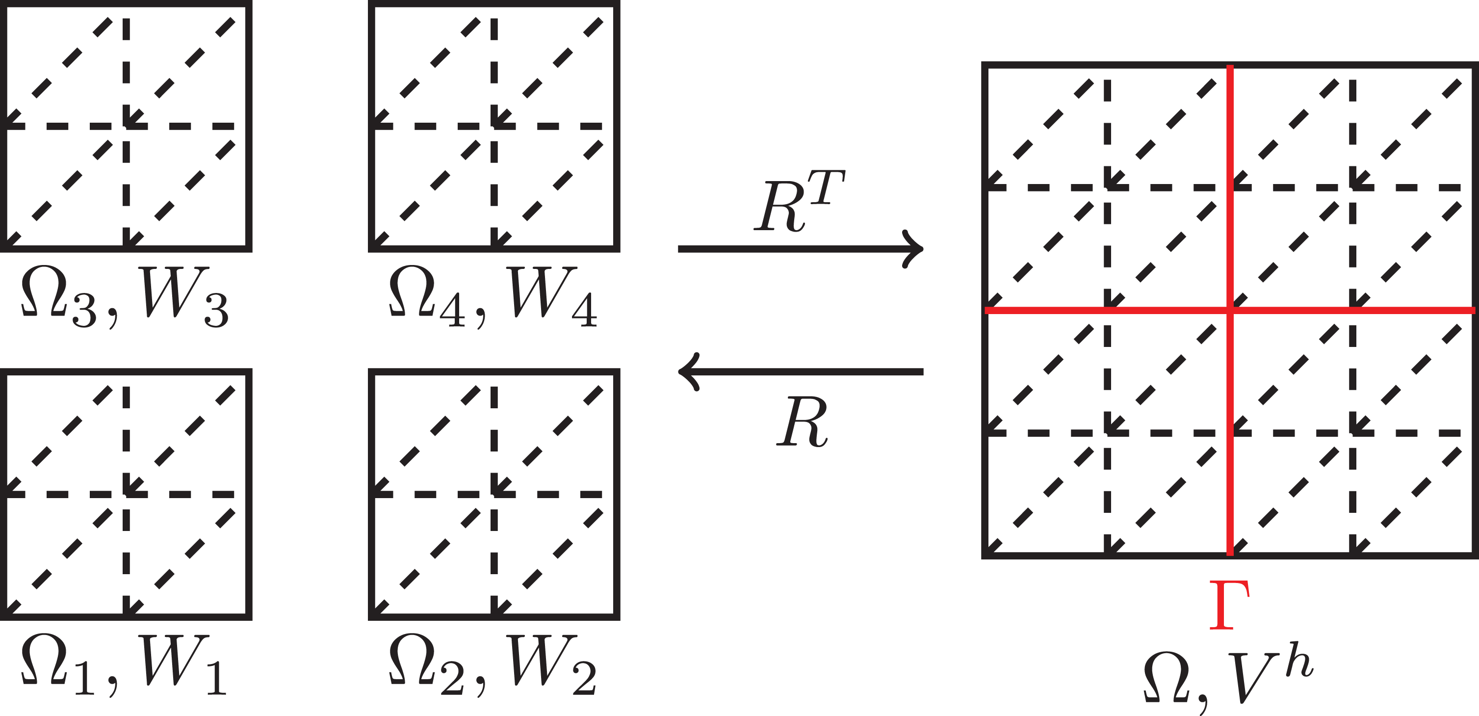
The application of RT
in eq. (8) and eq. (9) has thus the effect of a finite element assembly of local finite element functions on the interface
Let us assume, we have sorted and decomposed a solution u from the decoupled space

and

Enforcing continuity in the dual variables is done by enforcing
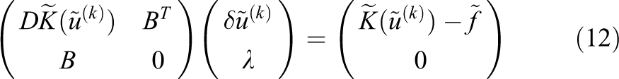
which is equivalent to eq. (7) and where λ is the vector of the Lagrange multipliers. Of course, several dual variables always belong to a common physical node on the interface and deliver more than a single entry in
By a block elimination in eq. (12) we derive the system
with

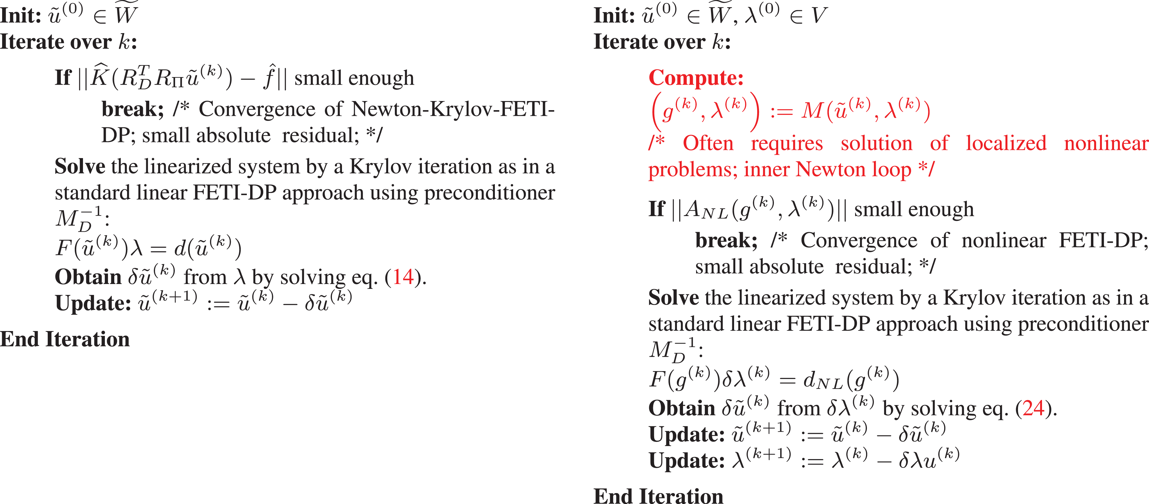
The complete Newton-Krylov-FETI-DP algorithm is also presented in Figure 5 (left).
2.2. The parallel application of F and the Dirichlet preconditioner
Solving eq. (13) iteratively, the matrix
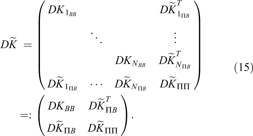
Since
For the construction of the Dirichlet preconditioner
2.3. Nonlinear-FETI-DP
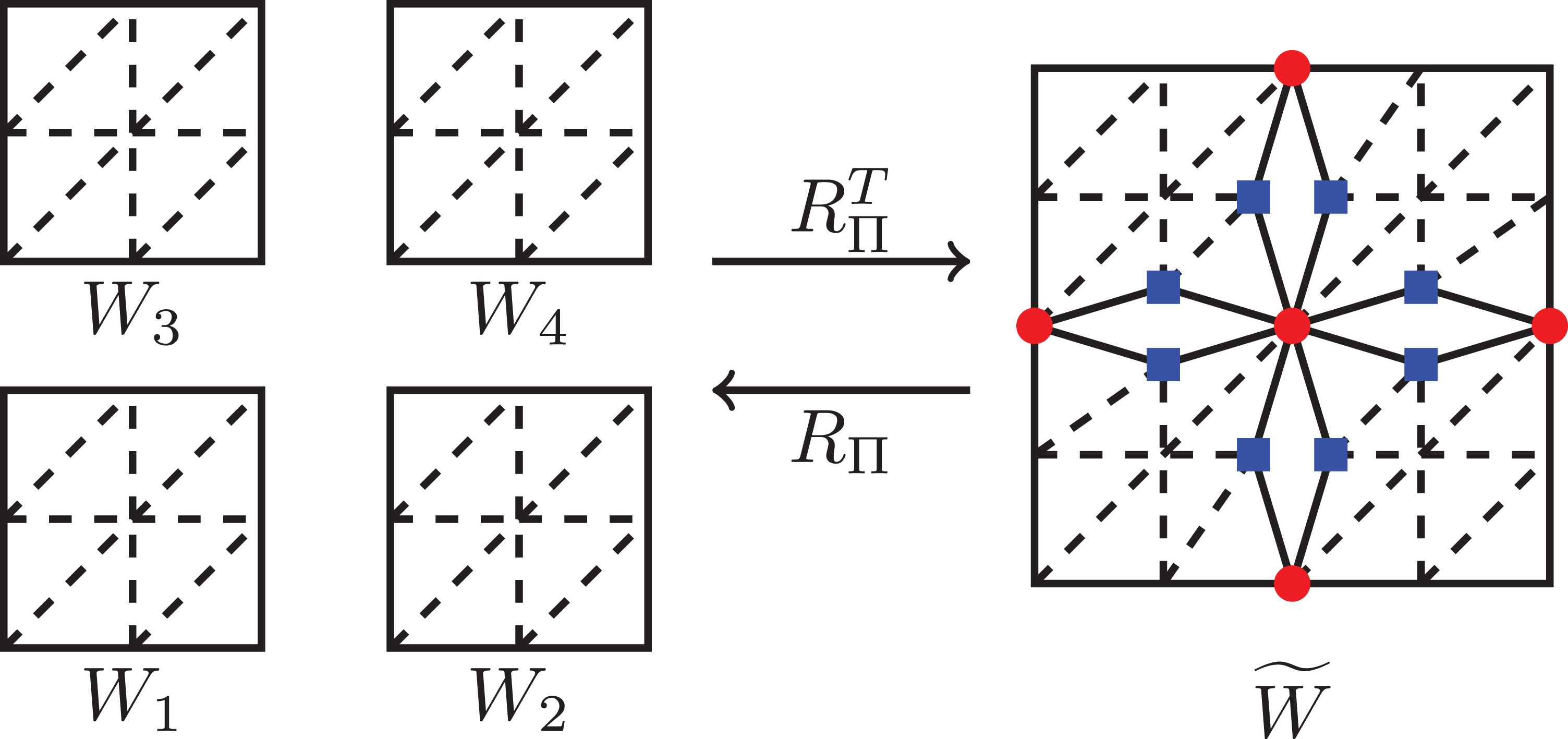
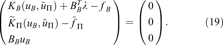
In the nonlinear FETI-DP approach, we first replace the nonlinear eq. (6) by a nonlinear saddle point formulation using ideas and operators from linear FETI-DP. With the nonlinear system from eq. (10), coupled in the primal variables, and enforcing the linear jump constraint
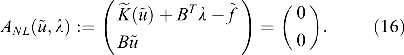
After applying a nonlinear right-preconditioner
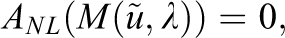
is solved by a Newton-Krylov method. We therefore obtain the solution by the iteration
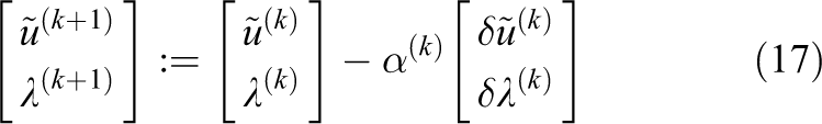
with the update defined by the linearized system
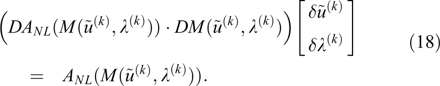
Different possible definitions of M are discussed in Klawonn et al. (2017), which all base on a partial nonlinear elimination of variables. It is shown in Klawonn et al. (2017) that eq. (18) can be solved using any linear FETI-DP approach and thus the linear solve in Newton-Krylov-FETI-DP and Nonlinear-FETI-DP only differs by the right hand side. Nonetheless, the preconditioner M has to be applied to
2.4. Nonlinear-FETI-DP-3
Using the index set
We now decide that the nonlinear preconditioner M is linear in

To evaluate the preconditioner, eq. (20) has to be solved by Newton’s method. Due to the completely decoupled block structure of KB
, the solution of eq. (20) collapses to local Newton iterations, one on each subdomain. The different Newton iterations on different subdomains are independent of each other. This process thus exclusively consists of local work. The nonlinear problems act on the red area marked in Figure 4 (middle) and the linearized systems with the tangential matrices

and
Finally, solving the linear system eq. (18) is equivalent to solving
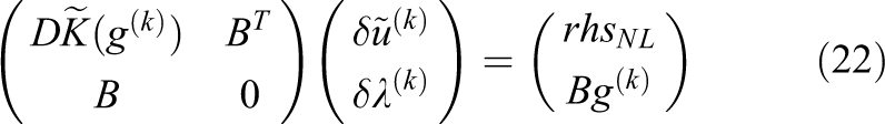
with
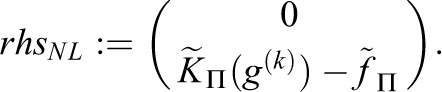
A proof can be found in Klawonn et al. (2017). Since the left hand sides in eq. (22) and eq. (12) have the same structure, any linear FETI-DP method can be used. As already described for Newton-Krylov-FETI-DP, we reduce the system to the Lagrange multipliers

with

An overview of the algorithm can be found in Figure 5 (right).
3. Nonlinear model problems
We choose nonlinear partial differential equations based on the p-Laplace operator with
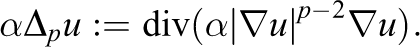
Our nonlinear model problem is now defined as
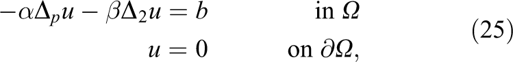
where

A restriction to a subdomain
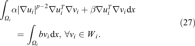
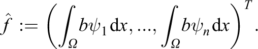
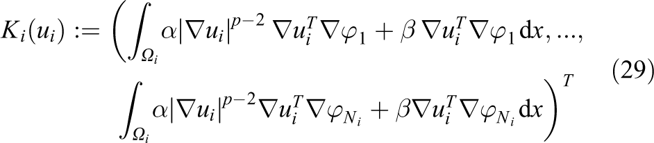
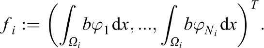
Therefore, given a finite element basis
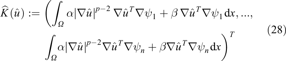
and
Restriction to a local finite element space Wi
, given a finite element basis
and
For the entries of the tangential matrices
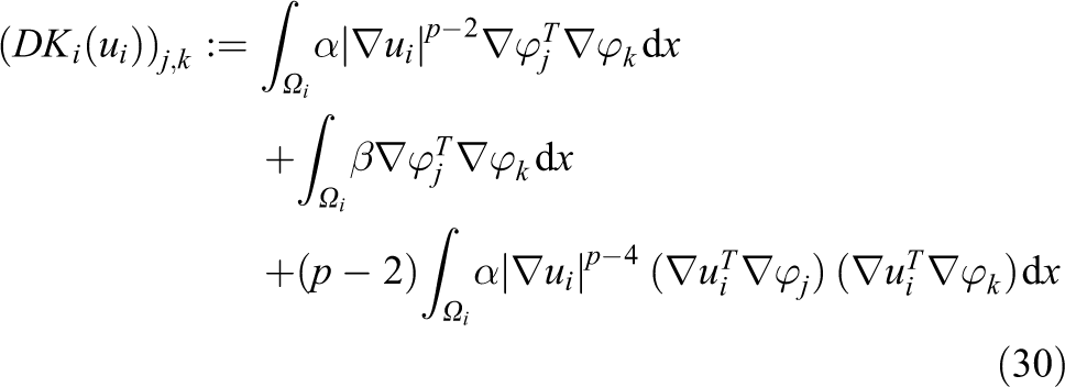
by a direct computation.
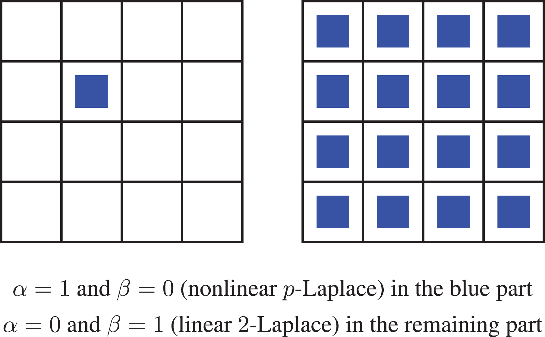
For the first configuration with a single nonlinearity, we consider a single inclusion of p-Laplace in a single subdomain and linear 2-Laplace in the remaining domain, i.e.
4. Reducing the energy consumption of nonlinear-FETI-DP
4.1. Related work and contribution
Reducing energy consumption of HPC applications has gained substantial attraction in the last decade. In the context of MPI several algorithms and runtime systems have been proposed (Hsu and Feng, 2005; Kappiah et al., 2005; Kerbyson et al., 2011; Lavrijsen et al., 2016; Li et al., 2010; Lim et al., 2011; Rountree et al., 2009; Vishnu et al., 2013), which typically follow the same idea: processes exhibiting a high slack time, i.e. time they are blocked with waiting for other processes or communicating, can be clocked down to save energy. This approach is used in Yang and Yang (2008) for an energy optimized barrier. Furthermore they propose a second optimization where the core waiting in the barrier is shutdown for a certain amount of time. However, they give no details in how this is established and how they obtain the energy measurements. A more fine grained approach is presented in Chen and Dong (2012), where certain algorithms for barrier synchronization are coupled with dynamic voltage and frequency scaling (DVFS) to save energy during the idle time.
Basically, we combine the idea of shutting down the core in the barrier with speeding up busy cores by accessing the power budget of the “barrier core” to scale up their frequencies. We propose a simple way to shut down cores entering barriers which are known to have sufficiently long wait times. The corresponding energy gains are measured for different nonlinear decomposition methods and the most important contributors to power consumption are investigated.
4.2. Energy reduction approach
In the following, we divide the cores into two classes. Cores, where the inner local Newton iteration, i.e. the evaluation of the nonlinear preconditioner M, converges fast, we call speeder, whereas the cores which must perform more inner Newton iterations we call laggers. All cores are synchronized with a barrier. Speeder cores arrive early and must wait for the laggers to arrive. The residence time of the speeders in the barrier is in the order of seconds for our nonlinear DD method and is visualized in Figure 7 for Newton-Krylov-FETI-DP (top row) and Nonlinear-FETI-DP-3 (bottom row). As expected, the load imbalance for Newton-Krylov-FETI-DP is insignificant for both model problems and there is no potential for a reduction of the energy consumption. In contrast, for Nonlinear-FETI-DP-3, the load imbalance is present for both model problems. Considering a
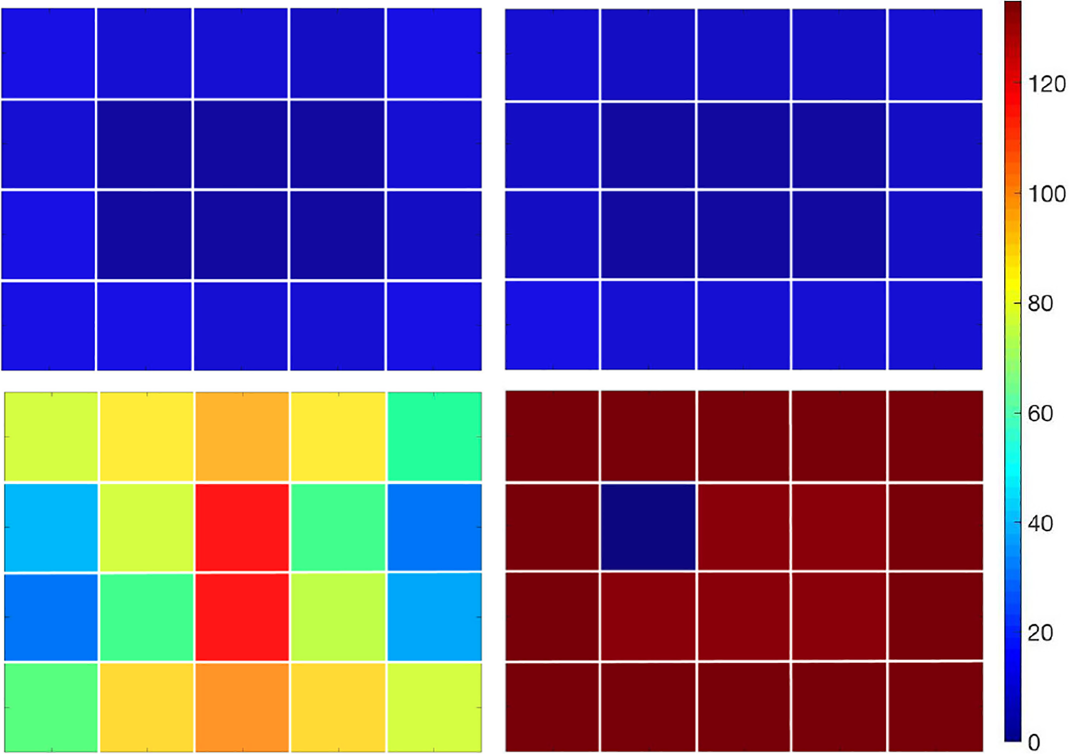
Time (given in seconds) of each core/subdomain spent in an MPI_Barrier. Example with 20 cores and subdomains on a single node.
As already mentioned, dynamic load balancing is currently not feasible. However, we can exploit the load imbalance to reduce the energy consumption of Nonlinear-FETI-DP-3. Here the typical approach for MPI applications is to clock cores down when they are either not in the critical path, i.e. their execution time does not affect the total runtime, or while they remain inside a barrier. This involves a runtime system determining the critical path or programmatically adjusting a core’s frequency. Both options are not practical as in most compute cluster production environments adjusting frequencies dynamically for selected cores is not allowed by users. Alternatively, one may rely on the Linux operating system which can adjust a core’s frequency automatically depending on the load. To do so a CPU frequency governor must be enabled. This governor is load driven and gracefully adjusts the frequency accordingly. However, we found that cores executing a barrier remained at their highest frequency and were not throttled by the governor. Such behavior is caused by the MPI progress engine when polling the fabrics for new messages. This leads to high instruction issue rates (see
Instead of reducing a speeder’s core frequency, a more effective strategy is to leverage a core’s (deep) sleep states. The operating system (OS), e.g. uses these states to save energy when cores are idle. This behavior can implicitly be triggered with current Linux kernels and a corresponding core by calling specific functions like
Non-blocking barrier with test-and-sleep loop as replacement for
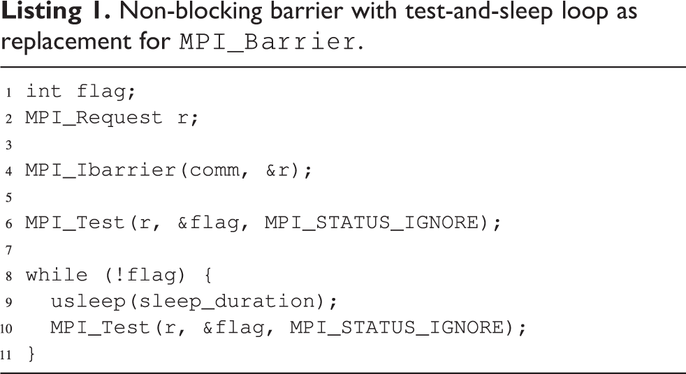
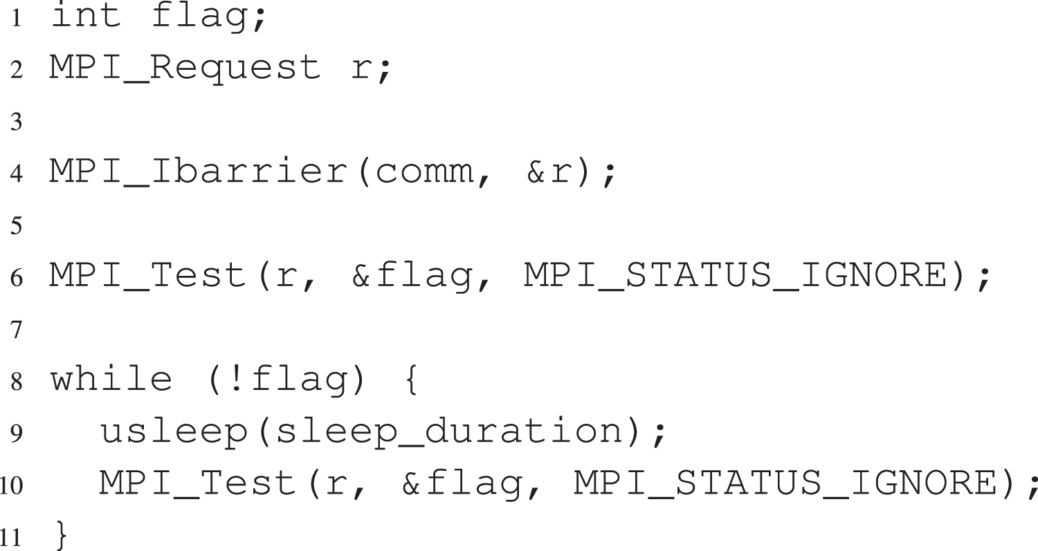
The correct choice of the duration for the sleep
An important side effect of sleeping cores is that laggers on the same chip have access to a higher fraction of the shared power budget of the chip. If DVFS is enabled they can increase clock speed and reduce their runtime. The more speeders are in deep sleep states, the higher laggers can be clocked and can potentially finish earlier.
4.3. Implementation remarks and testbed
All methods are implemented in PETSc (Balay et al., 2016a, 2016b) based on our nonlinear DD software (Klawonn et al., 2015) and using the same basic building blocks. Therefore, the timings and scaling results are comparable. We used PETSc version 3.6.4 and MKL-Pardiso from the MKL (Math Kernel Library) for all sparse direct solves. We refer to Klawonn et al. (2017) for a detailed description of our FETI-DP implementation.
We perform our experiments on the Linux-based Meggie cluster of the RRZE in Erlangen, Germany. All nodes are connected via Intel’s high speed 100 GBit Omni-Path network. One compute node consists of two Intel Xeon E5-2630 v4 processors with 10 cores each operating at a base frequency of 2.2 GHz. See Table 1 for further details on the compute node. Each processor has a thermal design power (TDP) of 85 W maximum (Intel Corp, 2016). However, the processor supports several features adjusting its power consumption which are briefly described in the following paragraphs.
Specifications of a Meggie compute node.
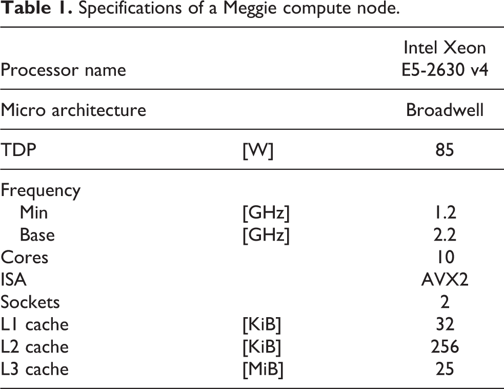
The processor supports DVFS which allows for dynamically adjusting each cores frequency individually. A core’s frequency can be as low as 1.2 GHz.
Furthermore, Intel’s Turbo Boost is supported and enabled. This technique allows for dynamically overclocking a core as long as the chip stays inside its power envelope and does not exceed certain thermal constraints. The maximum clock speed depends on several factors like the temperature of the processor, the current workload, and the number of active cores.
Table 2 lists the maximum Turbo Boost frequencies depending on the number of active cores (Intel Corp, 2016). Note that these frequencies specify only an upper limit and might be lower because of the previously named reasons.
Maximum turbo frequency in GHz depending on the number of active cores for the Intel Xeon E5-2630 v4 processor according to Intel Corp (2016). Reported frequencies specify an upper limit and can be lower depending on e.g. current power consumption or temperature.
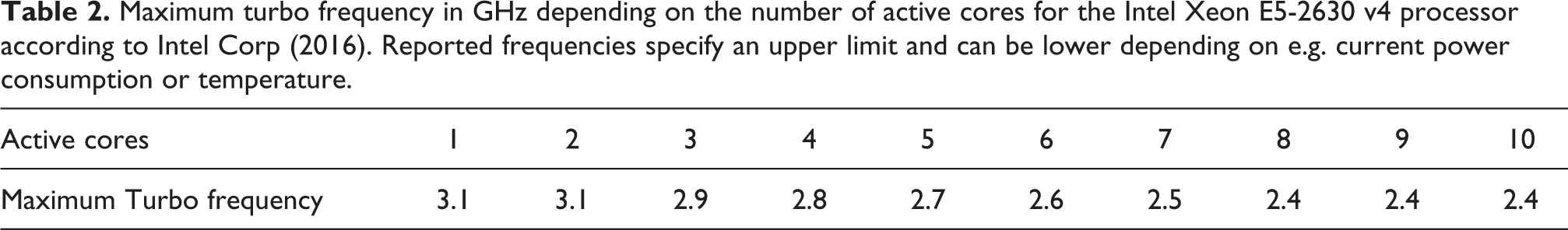
A core executing AVX workloads, precisely executing 256 bit AVX instructions, gets its frequency dynamically reduced to the so called AVX frequency. If, for a certain amount of time, no AVX 256 bit instruction was encountered the core’s frequency is raised back again to the non-AVX frequency. For the processor model used, it seems that Intel does not provide detailed information about the AVX frequencies. Only Microway (2018) lists 1.8 GHz as the base AVX frequency and 3.1 GHz as the highest AVX Turbo Boost frequency.
For advanced energy saving, each core supports (deep) sleep states, also known as C-states. A state higher than the normal operating state C0 denotes a core as inactive and thus requires less power. The power consumption decreases with increase in the sleep state level. The processor used supports four states namely C1, C1E, C3, and C6, where the last one denotes the deepest one.
The cluster runs CentOS with Linux kernel 3.10-862. The CPU frequency governor which adapts the clock frequencies is in “conservative mode” on all Meggie nodes. The Intel C/C++ compiler “17.0 update 1” and the Intel MPI library version “2017 update 1” was used. We used the likwid tool suite (Treibig et al., 2010) to measure performance, power and clock speeds. To determine power and energy consumption likwid uses the Intel running average power limit (RAPL) interface which delivers data of high quality (Hackenberg et al., 2015). All energy numbers and power consumption measurements include the contributions of the processor chip(s) and the main memory. No other devices are monitored (e.g. power supply or networks).
At the time of the first installation of Meggie the true power consumption of the complete cluster was measured. A consumption of 210 kW was observed while performing the linpack benchmark, 65 kW when the cluster was idle, and still 7 kW when the cluster was in the power down state, i.e. with active management cards. Therefore, the energy saving potential due to algorithms and software is up to 145 kW for Meggie, i.e. approximately 70% of the power consumption is due to algorithm and software. The discussion on energy savings in this paper refers to this portion of the energy consumption. We do not include the power consumption of main memory as its maximum contribution to overall power was always below 10%.
4.4. Single node measurements
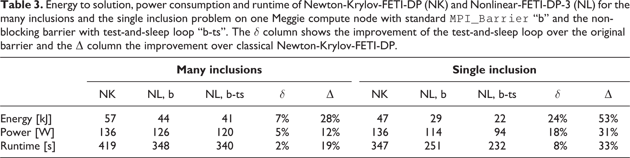
Measurements of Newton-Krylov-FETI-DP and Nonlinear-FETI-DP-3 with the standard
Energy to solution, power consumption and runtime of Newton-Krylov-FETI-DP (NK) and Nonlinear-FETI-DP-3 (NL) for the many inclusions and the single inclusion problem on one Meggie compute node with standard
For a more detailed analysis of Nonlinear-FETI-DP-3, we performed time-resolved measurements. While executing the code, we measure the average core frequency using likwid (Treibig et al., 2010) (averaging interval is 1 s) and we determine the fraction of time spent in the deepest sleep state C6 in each interval (using the cpu_idle driver). Figure 8 shows the time-resolved plot for both model problems on a full node of Meggie using 20 cores. Whenever no core is in C6 state (lower panels in Figure 8), all cores achieve the maximum turbo frequency of 2.4 GHz for fully loaded sockets (see upper panel in Figure 8). However, if speeders are entering sleep states they make room for overclocking of the laggers. If some cores’ frequencies go down to 1.2 GHz and their fraction of time spent in C6 state is close to 100%, the remaining cores get a boost in clock speed. A nice side effect of the measurements presented in Figure 8 is that one can read out the structure of a typical application of a nonlinear domain decomposition method: An inner iteration, where—one after another—the cores run into some synchronization point followed by a linear solve, where all cores participate with similar effort. For example, for the
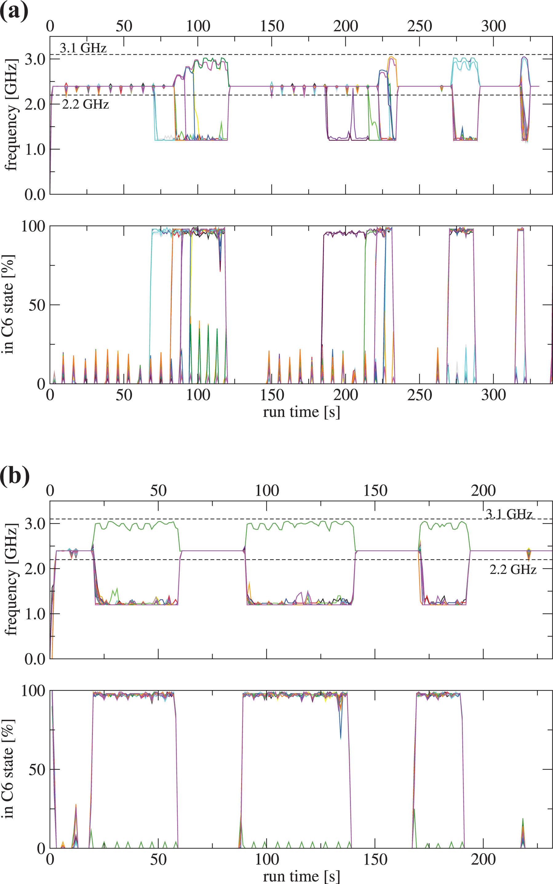
Time-resolved execution of the Nonlinear-FETI-DP-3 algorithm with the test-and-sleep barrier for the many inclusions (a) and the single inclusion problem (b) for each of the 20 cores of a Meggie (different colors) compute node.
Depending on how many cores are already sleeping, i.e. how many cores have finished the inner loop, the processor core frequency is raised to around 3.0 GHz according to the graphs. Even in the case of only a single inclusion in Figure 8b, where only one lagger is present, it seems that the possible 3.1 GHz Turbo Boost frequency is not reached exactly. Several reasons may account for that slight deviation, e.g. the finite length of the averaging interval and the frequent wake ups of the speeders to check for barrier progress.
The measurements in Figure 8 indicate a frequency of 1.2 GHz for cores spending nearly their complete fraction of the 1 s averaging intervals in a deep sleep state. During that time cores are effectively halted and they reduce clock speed down to (almost) zero. The reported value is an artifact of the finite averaging interval being much longer than the sleep states (10 ms). In such scenario likwid reports the clock speed of the core when it wakes up for barrier testing which is done at the lowest possible frequency of 1.2 GHz.
4.5. Multi node measurements
For multi node measurements, we employ weak scaling by doubling the number of subdomains in each spatial dimension. Note that the problem with the
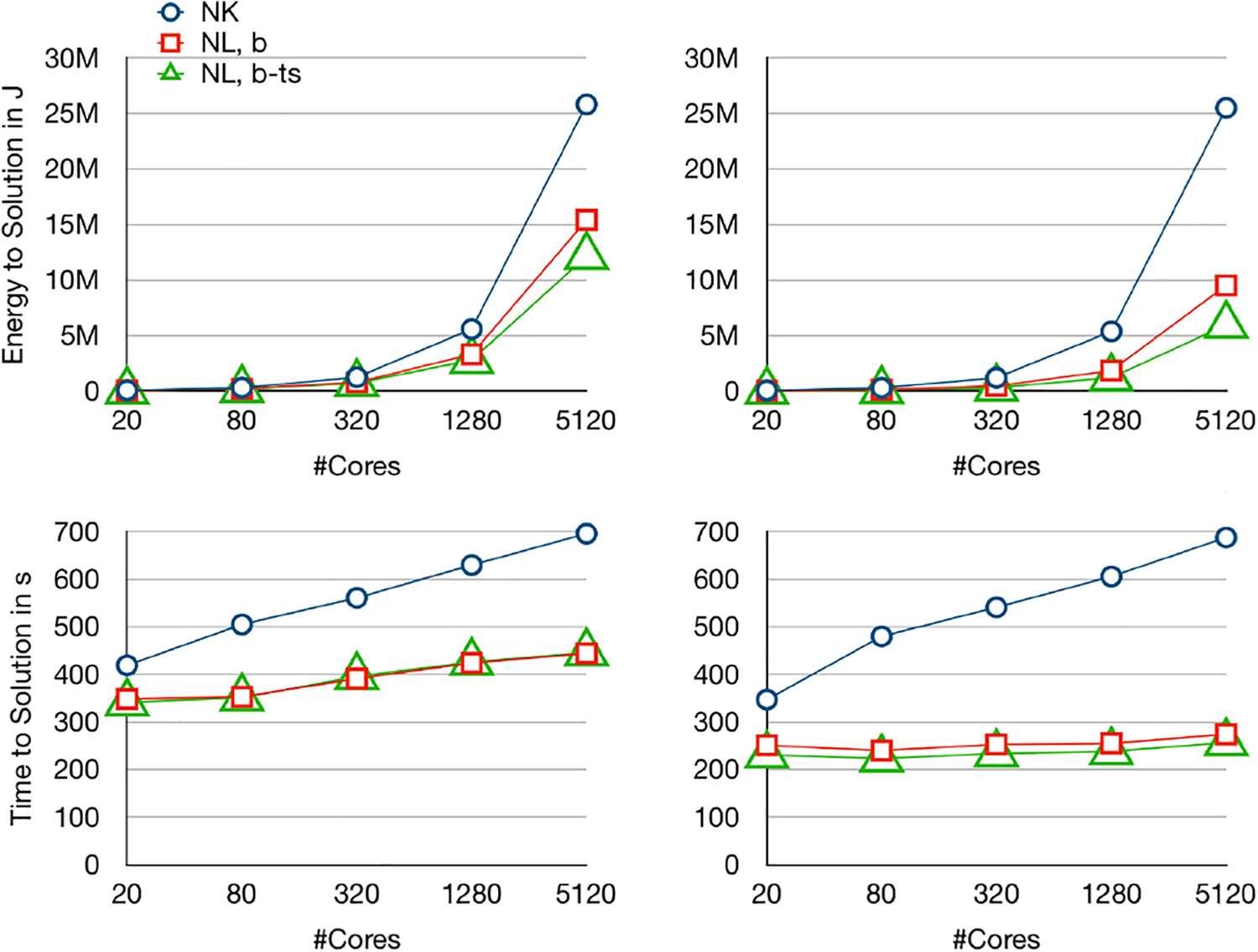
Total energy consumption (top panels) and runtime (bottom panels) of Newton-Krylov-FETI-DP and Nonlinear-FETI-DP-3 for both model problems—
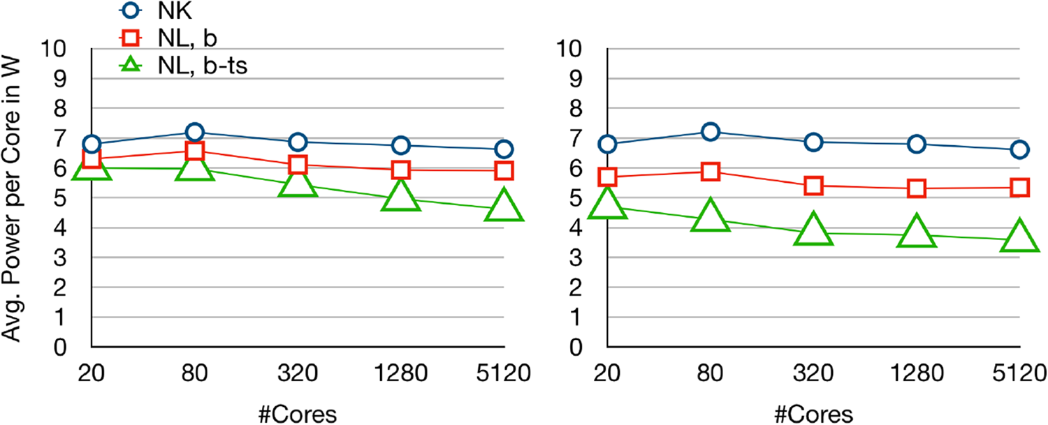
Average power consumption per core of Newton-Krylov-FETI-DP and Nonlinear-FETI-DP-3 for two model problems—
Let us note that the power per core is even decreasing during the weak scaling study as with increasing core counts barrier time increases. This characteristic increase of barrier time in overall runtime emphasizes the need for power efficient barriers in large scale computations. Thus, in our study, the effect of the test-and-sleep barrier is more significant on 256 nodes than on a single node. Here, the energy per core is reduced by 23% for the
4.6. Other solvers
To illustrate that the concepts introduced here can be carried over to other nonlinear domain decomposition methods besides Nonlinear-FETI-DP-3, we briefly present some single node measurements for ASPIN (Additive Schwarz Preconditioned Inexact Newton) (Cai and Keyes, 2002). We therefore use the ASPIN implementation available in PETSc (Balay et al., 2016a, 2016b) and the p-Laplace example provided by PETSc as ex15.c; see Brune et al. (2015, section 6.5) for details. Let us remark that in ex15 finite differences are used instead of finite elements. Written in our notation from section 3, we have
For a detailed description of ASPIN, we refer to Cai and Keyes (2002). Let us just remark that ASPIN is a nonlinearly left-preconditioned method and that the nonlinear preconditioner reduces to independent nonlinear Dirichlet problems on overlapping subdomains.
The ASPIN solver exhibits a load imbalance as shown in Figure 11 when evaluating the nonlinear preconditioner. In contrast to our FETI-DP implementation, where the time was spent in barriers, here the imbalance is visible through long waiting times in
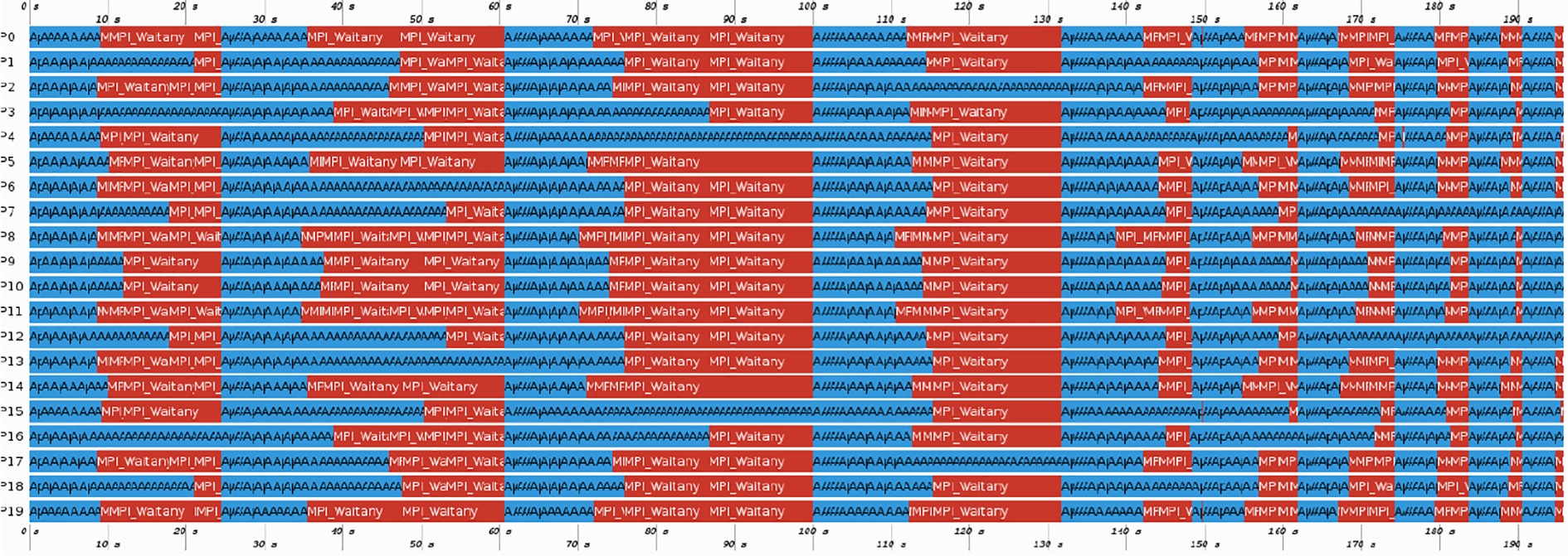
Trace of ASPIN obtained with Intel Trace Analyzer on one Meggie node. Blue bars denote time spend in application, whereas red bars denote time spend in MPI; here predominantly MPI_Waitany.
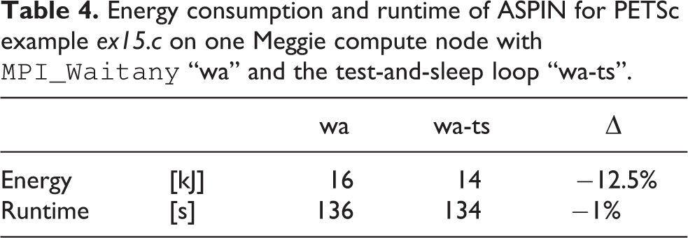
The energy consumption and runtime for the wait and test-and-sleep cases are reported in Table 4. As for Nonlinear-FETI-DP-3, test-and-sleep reduces the energy consumption by 14% and has no negative impact on the performance.
Energy consumption and runtime of ASPIN for PETSc example ex15.c on one Meggie compute node with
5. Analysis of basic power contributions
In a final step we make sense of the power measurements presented in Figure 10 by low level benchmarking and simplistic power modeling. We choose the single inclusion scenario in the limit of large processor counts to identify the relevant power contributions. For the Nonlinear-FETI-DP-3 method this is the extreme case where only one processor is computing throughout while the remaining ones execute the standard barrier or its test-and-sleep replacement most of the time. Thus, overall power consumption will be determined by executing the standard barrier or the baseline power of the processors being in sleep state. For the Newton-Krylov-FETI-DP method time to solution and power consumption will be mostly governed by computation and it can serve as a reference for the power contributions of computations of all methods considered in this paper. To separate these effects we first run several benchmarks on full sockets (10 cores) and report their power consumption and power variation across 500 sockets in Figure 12:
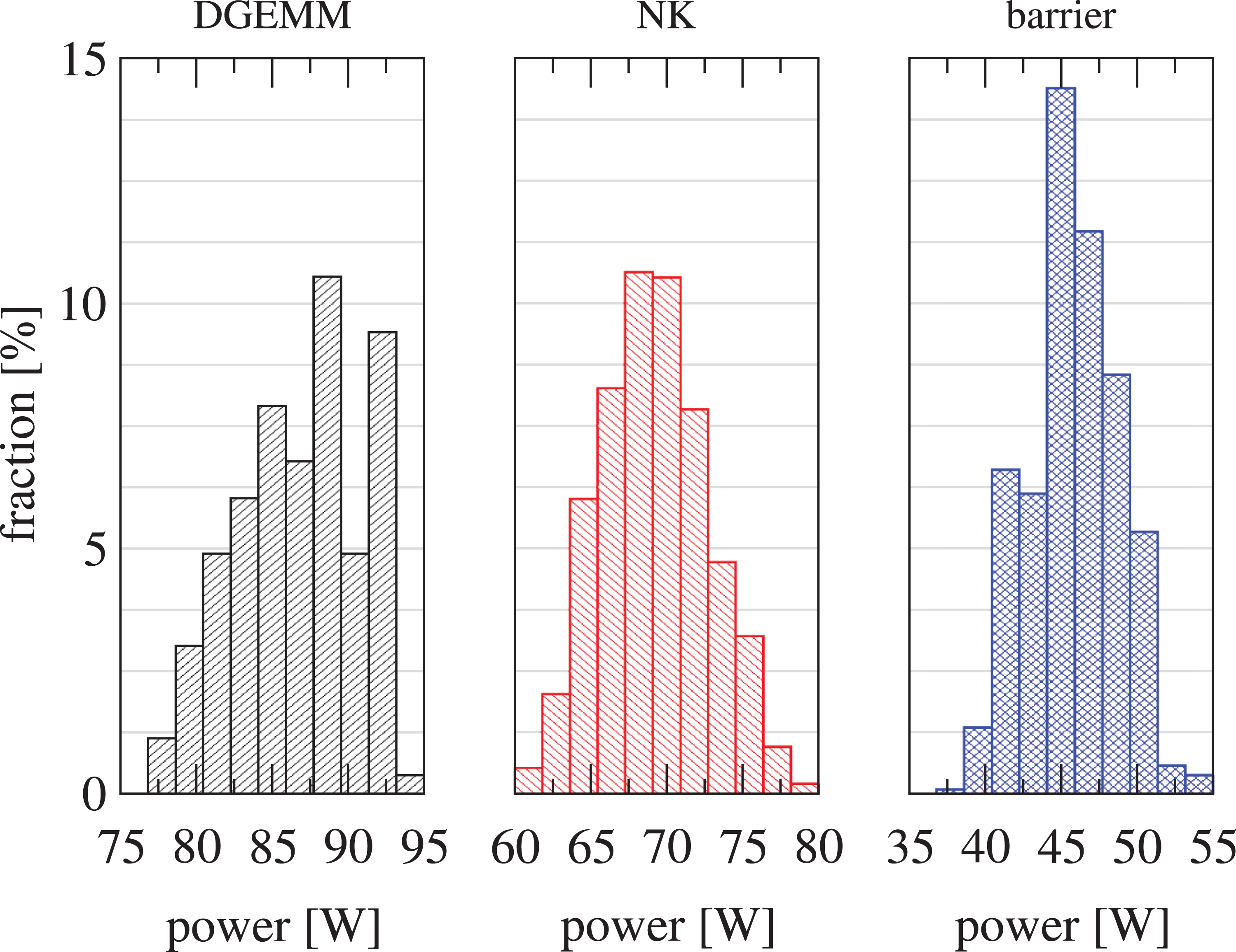
Distribution of power consumption of processors and their associated memory from the Meggie cluster under different workloads: DGEMM, Newton-Krylov (NK), and barrier. Note the different scaling on the x axis.
In addition we provide measurements for dense matrix matrix multiplication (using DGEMM from Intel mkl) which is considered to be an upper limit for application power consumption. Note, it is not sufficient to measure a single chip as there can be a substantial power variation between different chips of the same processor type running at the same clock speed (Inadomi et al., 2015; Rountree et al., 2012). Accordingly, for all benchmarks we find substantial power fluctuations across the processor chips in our compute cluster (see Figure 12). The different power levels drawn by these three corner cases directly relate to their hardware utilization as confirmed by likwid measurements for typical hardware utilization metrics such as instruction throughput (IPC) and cache/memory bandwidths. The
In a final step we attempt to understand the power level of Nonlinear-FETI-DP-3 with our test/sleep barrier implementation (approx. 3.6 Watt/core; single inclusion in Figure 10). We expect that this barrier implementation should have marginal power contributions as the idle cores are in a deep sleep state. Here, the baseline power of the chip

where
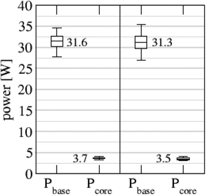
Fitted values of base
Our results clearly substantiate the potential high impact of standard barrier implementations on power consumption of applications inhibiting load imbalances. As future architectures are expected to be more dynamic in terms of power consumption including lower baseline powers, the need for power efficient implementations of solvers and barriers will increase accordingly.
6. Conclusion
We have shown that nonlinear DD methods can reduce the energy consumption, compared to standard Newton-Krylov-DD approaches, first by a reduction of time to solution, and, additionally, by a better power efficiency.
For nonlinear DD methods the efficiency can be improved further by using a nonblocking barrier and actively setting cores to sleep mode.
For the example of Nonlinear-FETI-DP-3 and different model problems, energy savings up to 77% can be reached, as measured by the RAPL hardware counter, without affecting the runtime. The concepts introduced in this paper can be easily carried over to many nonlinear DD approaches, as, e.g. ASPIN or nonlinear BDDC, and can be combined with approaches to reduce the load imbalance.
Footnotes
Acknowledgements
The authors gratefully acknowledge the compute resources granted on Meggie and support provided by the Erlangen Regional Computing Center (RRZE).
Declaration of conflicting interests
The author(s) declared no potential conflicts of interest with respect to the research, authorship, and/or publication of this article.
Funding
The author(s) disclosed receipt of the following financial support for the research, authorship, and/or publication of this article: This work was supported by the German Research Foundation (DFG) through the Priority Programme 1648 “Software for Exascale Computing” (SPPEXA) in the DFG projects 230723766 (EXASTEEL II) and 230898523 (ESSEX II).