
Abstract
Smoothed particle hydrodynamics (SPH) method is widely accepted as a flexible numerical treatment for surface boundaries and interactions. High-resolution simulations of hydrodynamic events require high-performance computing (HPC). There is a need for an SPH code that runs efficiently on modern supercomputers involving accelerators such as NVIDIA or AMD graphics processing units. In this work, we applied half-precision, which is widely used in artificial intelligence, to the SPH method. However, improving HPC performance at such low-order precisions is a challenge. An as-is implementation with half-precision will have lower computational cost than that of float/double precision simulations, but also worsens the simulation accuracy. We propose a scaling and shifting method that maintains the simulation accuracy near the level of float/double precision. By examining the impact of half-precision on the simulation accuracy and time-to-solution, we demonstrated that the use of half-precision can improve the computational performance of SPH simulations for scientific purposes without sacrificing the accuracy. In addition, we demonstrated that the efficiency of half-precision depends on the architecture used.
Keywords
1. Introduction
Smoothed particle hydrodynamics (SPH) (Lucy 1977; Gingold and Monaghan 1977) method is a widely accepted particle-based numerical hydrodynamical scheme. SPH was first developed for use in the field of astrophysics to simulate the fission of protostars. Its use has since expanded to disaster prevention (Heller and Spinneken 2015; Wang et al. 2016), engineering (Crespo et al. 2008; Lee et al. 2010), and geosciences (Nakajima and Stevenson 2015; Rufu et al. 2017; Hosono et al. 2019). Unlike grid-based methods, SPH can handle systems with large deformations, moving boundaries, and interactions with structures. Large-scale and/or high-resolution SPH simulations are highly demanded.
A major disadvantage of SPH over grid-based methods is its high computational cost. The SPH method represents a fluid as a collection of SPH particles and converts the governing equations, such as the equations of continuity and motion, into sums of interactions between these particles. The computational cost of these implementations grows as O(N2) (where N is the number of SPH particles). Such high computational cost prevents the large-scale and/or high-resolution numerical simulations of SPH; the cost must be reduced through high-performance computing (HPC) techniques.
Since June of 2022, many supercomputers listed on the TOP500 and/or GREEN500 have been identified as GPU supercomputers. Hence, parallel SPH algorithms that work effectively on distributed parallel GPU systems are urgently required.
The computational cost of an algorithm is commonly reduced by compiling a neighbor list. A naive construction of an interaction list costs O(N2). Among various techniques in which neighbor lists are constructed faster than O(N2), we selected the tree method (e.g., Hernquist and Katz 1989) that utilizes the spatial octree structure the search neighbor particles. First, we set a cell that involves all particles. Then, the cell is divided divide it into eight daughter cells. This process is performed recursively until all the cells contain less than a certain number of particles. Then, by traversing obtained tree structure, we constructed neighbor lists. This can reduce the computational cost to O(N log8N).
In addition to reducing the cost of creating neighbor lists, we must also reduce the cost of calculating the interparticle interactions. The force calculation can be accelerated by a technique called half-precision, which is widely employed in artificial intelligence (AI) libraries (e.g., TensorFlow and PyTorch). Processors such as NVIDIA graphics processing unit (GPU) and Fujitsu A64FX that support arithmetic operations were recently developed. Half-precision halves the computational cost from that of single-precision and has already been applied to mesh methods (Klöwer et al. 2022, and references therein).
Although half-precision reduces the cost of the force calculation, it can worsen the simulation accuracy. Therefore, it is unclear whether half-precision is consistently effective in scientific simulations. Because accuracy is of paramount importance in scientific simulations, any accuracy degradation must be addressed by deploying more particles, thereby lengthening the time-to-solution. This requirement may render half-precision useless for scientific purposes. Therefore, the viability of half-precision is determined by the balance between the simulation accuracy and the acceleration. Although several prior works have reduced the precision of SPH (e.g., Zhang et al. 2008; Nakasato et al. 2012; Saikali et al. 2020), they did not address the tradeoff between accuracy loss and speedup.
In this work, the effectiveness of half-precision for scientific purposes was examined. We first introduced half-precision to the force calculation of SPH. Because a straightforward implementation of half-precision to SPH may worsen the accuracy, we develop a practical implementation that mitigates the accuracy loss resulting from half-precision. Based on the mixed-precision technique (e.g., Micikevicius et al. 2017; Abdelfattah et al. 2021), our method implements all procedures other than the force calculation (e.g., the creation of neighbor lists and time integration) in double precision on CPUs. We truncated the double-precision variables to single- or half-precision before computing the interparticle interactions for the force calculation. The forces are calculated in GPUs (e.g., Hosono and Furuichi 2019) and stored in single- or half-precision until the force calculation is completed. Thereafter, they are reverted to double precision. Note that our methodology requires persistent offloading between the host memory and device memory. Offloading is advantageous for dynamic load balancing and parallel domain decomposition (e.g., Hamada et al. 2009) in the massively parallel distributed memory systems found in the TOP500 supercomputers. Although a fully native implementation can reduce the cost of communication between the host and device memory in accelerators, such as GPUs, it is technically difficult to achieve with advanced parallel dynamic load balancing modules over MPI. Therefore, we adopted offloading. An example code of our presented scheme is available at https://github.com/NatsukiHosono/WeaklyCompressibleSPH. The offloading restriction will be resolved in future GPU systems that have memory coherent with the CPU.
To derive the estimated time-to-solution, we considered the balance between the simulation accuracy (i.e., the simulation error (Monaghan 2005; Price 2012; Zhu et al. 2015)) and the cost of the force calculation. We then derived the conditions under which half-precision is effective for SPH simulations.
Among the several available versions of SPH, we selected the SPH of weakly compressible viscous flows (Monaghan, 1994, 2006). As test problems, we selected the two-dimensional (2D) Couette flow and a three-dimensional (3D) dam-break test. These problems are commonly used as benchmarks in studies on weakly kinematic viscous flows. The accuracy and speedup of SPH were checked for different particle numbers and floating-point precisions. From the results, we assessed the effectiveness of half-precision for the two problems.
The problems were solved on two GPU + CPU systems (NVIDIA V100 + Intel Xeon Gold and NVIDIA A100 + AMD EPYC 7742) and a CPU system (A64FX). The GPU + CPU systems are frequently listed in TOP500 and GREEN500, and the CPU system was listed second in the TOP500 (as of June 2022).
The remainder of this paper is organized as follows. Section 2 briefly summarizes the SPH method and then describes the introduction of half-precision techniques to SPH. In Section 3, the conditions under which half-precision effectively reduces the time-to-solution is derived. Section 4 deals with the implementation of our half-precision SPH on the aforementioned systems. We also describe the timing model of our implementation. Section 5 presents the setup of the 2D Couette flow and 3D dam-break test. Section 6 presents our timing measurements and simulation errors. Our findings are summarized in Section 7.
2.Method
This section briefly reviews SPH for weakly kinematic flows (a detailed description is given in (Monaghan 2006)).
2.1.SPH (smoothed particle hydrodynamics)
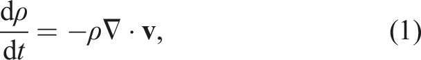
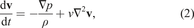
The continuity and motion equations of weakly compressible flows are, respectively, given as follows
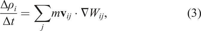
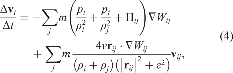
In the standard SPH method, these equations are formulated as follows

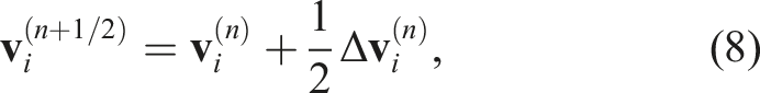
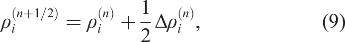
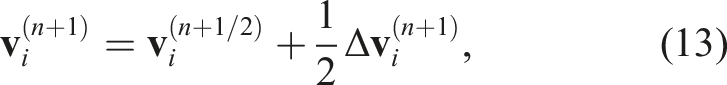
Time integration was performed using the second-order Runge–Kutta scheme (Cullen and Dehnen 2010; Hosono et al. 2016). The procedure of the (n)-th step can be summarized as follows. First, the velocity and density at half step are computed

Subsequently, the velocity and density at the next step are predicted


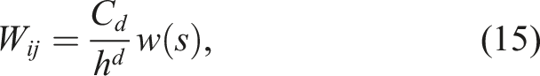
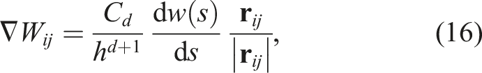
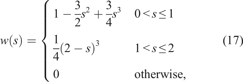
By using

The function W is the “kernel function” indicating the weight for each interaction (for details, see (Dehnen and Aly 2012)). We chose the simplest function of W, namely, the cubic spline function
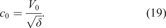
The pressure p is given by the equation of state. The following equation of state (Monaghan 1994) is widely used for weakly compressible flows
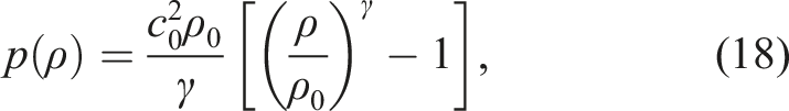
The parameter δ adjusts the compressibility until the time step is a reasonable size. Throughout this study, we set δ = 0.01.
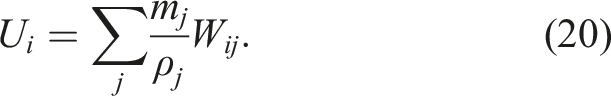
Shepard filtering (e.g., Crespo et al. 2011; Rosswog 2015; Di G. Sigalotti et al. 2016) with a Shepard-type partition of unity (Shepard 1968) has been commonly used to recover from density fluctuations. In this filtering process, we first calculate the following quantity, which should be unity
The density ρ
i
is then replaced by
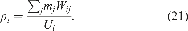
The above filter is applied at 30-step intervals and executed with double precision on the host CPU.
The overall procedure of the SPH method is executed as follows:
Step 3 is the most computationally intensive step as it involves double sweeps of particles. Therefore, Step 3 was the focus of our speedup process. The technical approach of Step 3 is described in Section 4.
2.2. Scaling and shifting
Largest normal numbers and numbers of exponent and fraction bits as defined by IEEE-754 for the three floating-point precisions.
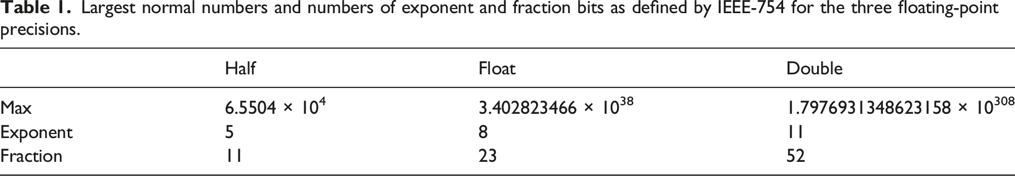
To provide a basis for scaling, the characteristic density ρ0, velocity V0, and length L are first defined within the setting of the target problem (e.g., fluid density, speed, and size of the domain boundaries). Accordingly, the pressure and kinematic viscosity are normalized as
By substituting equation (16) into equation (4), we get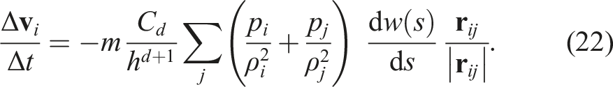
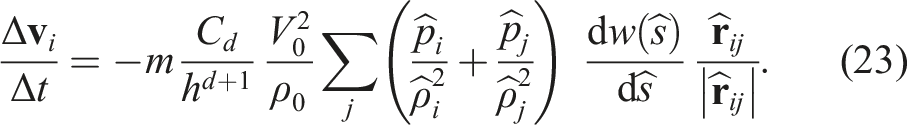
These procedures are necessary for stabilizing the half-precision runs. Since half-precision has a small representative range, a small value is rounded to zero. The scaling technique mitigates this issue by scaling all variables truncated to half-precision to O (1).
We then shift the particle positions to express their relative positions efficiently. Because the j-particles interacting with the i-particles are neighbors, the scaled j-particle position is shifted as follows
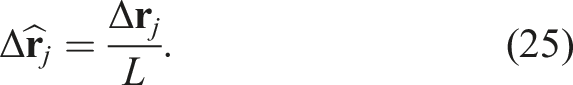
Using equation (25), we have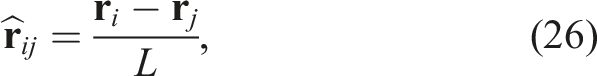
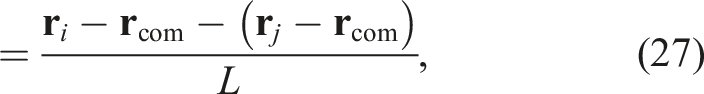
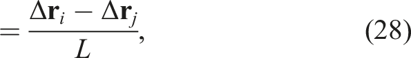

Replacing 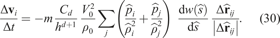
The scaling and shifting procedures were also applied to the relative velocity vector for the low-precision computations of equations (3)–(7). Hence, in addition to knowledge the center of mass of all the i-particles in a particle group, we also need to know its velocity. The center of mass and velocity are calculated when the tree structure is constructed with double precision.
Note that our shift operation moves global coordinates to the reference frame with the center of mass of each particle group. Unlike arbitrary Lagrangian–Eulerian adjustments, our shift does not rearrange the particle positions.
Although
In this study, we emphasize that the scaling and shifting techniques are the requirements from the low precision. Although the scaling technique is commonly used in the field of computational fluid dynamics, in many cases, it is used for numerical stability with float or double precision (Darwish (1993) and references therein).
3. Simulation accuracy versus speedup
This section describes the derivation of the conditions necessary for determining the usefulness of half-precision in SPH simulations. To this end, we estimated the time-to-solution by balancing the accuracy and speedup.
First, we estimated the timestep size Δt as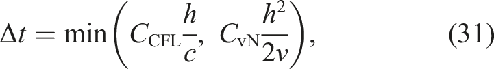
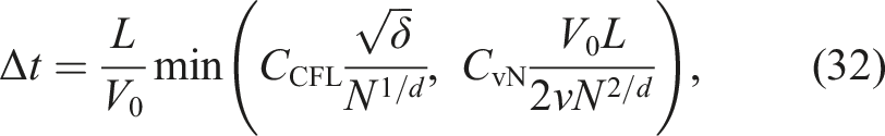
In many-particle cases, the latter term pf the above expression is greater than the former term. Hence, we focused on the latter term.
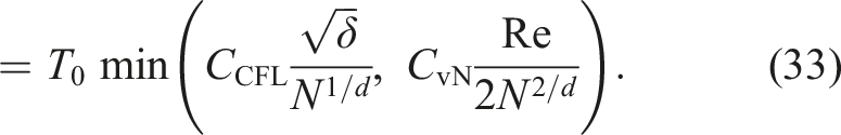
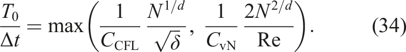
The time-to-solution 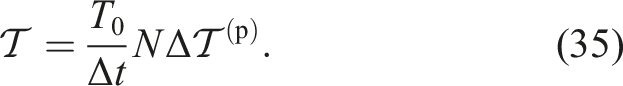
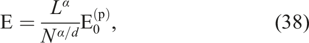
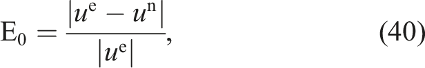
Next, let us consider the error. The error E in SPH can be predicted as
The actual choice of E0 depends on the problem. If the problem can have an analytical solution, many researchers (e.g., Song et al. 2018) adopt the L2 error, which is defined as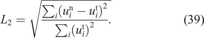
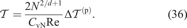
By combining equations (36) and (38), we can obtain the “balance” between the accuracy (error) and the time-to-solution. Using equation (38) to eliminate N from equation (36), we obtain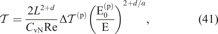
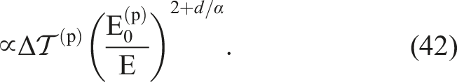
Recall that if the half-precision is effective for scientific purposes, 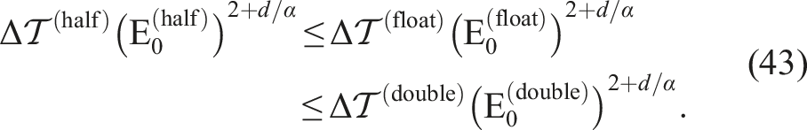
Note that in 3D problems, d is 3 and α is (ideally) −2. Hence, in 3D problems, we have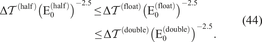
Recall also that
We should not merely assume the truth of equation (38) in actual simulations. The error convergence of SPH is assured only when the particles are well ordered, whereas in actual simulations, the particle configurations become disordered because of the inherent nature of SPH formulations and may be imprecise. To check whether the convergence behaviors hold, we changed the precisions and numbers of particles in the two well-known test problems.
Next, we describe our half-precision implementation in SPH and measurements of the wall-clock time
4. CPU/GPU Implementation
We tested two types of systems, namely, a CPU-only system and CPU + GPU systems. In the CPU-only system, all the steps in the overall procedure described in Section 2.1 were performed on the CPU. In the CPU + GPU systems, Step 3 was mainly performed on the GPUs. For this purpose, we adopted the so-called “multiwalk” method (Hamada et al. 2009), which was first developed for performing efficient gravitational N-body simulations on GPUs. This has recently proven effective in the SPH method (Hosono and Furuichi 2019). The multiwalk method begins with a group of i-particles. A neighbor list containing all neighboring particles of each i-particle in the group is then created. The multiple groups and their neighbor lists are sent to a GPU for the force calculation. Step 3 is divided into the following substeps: Step 3.1: Scale and shift the data of each particle group (and its neighbor list). Step 3.2: Convert the data type from on-host to on-device. This substep truncates the on-host data type (double) to the on-device data type (float/half). Step 3.3: Send the data to the accelerator. Step 3.4: Invoke the force calculation. Step 3.5: Receive the results from the accelerator. Step 3.6: Convert the force from the on-device data type (float/half) to the on-host data type (double).
The neighbor lists were created using the Framework for Developing Particle Simulator (Iwasawa et al. 2016, 2020).
With this implementation, we can categorize
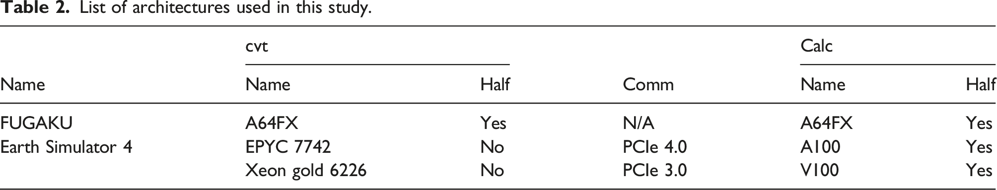
List of architectures used in this study.
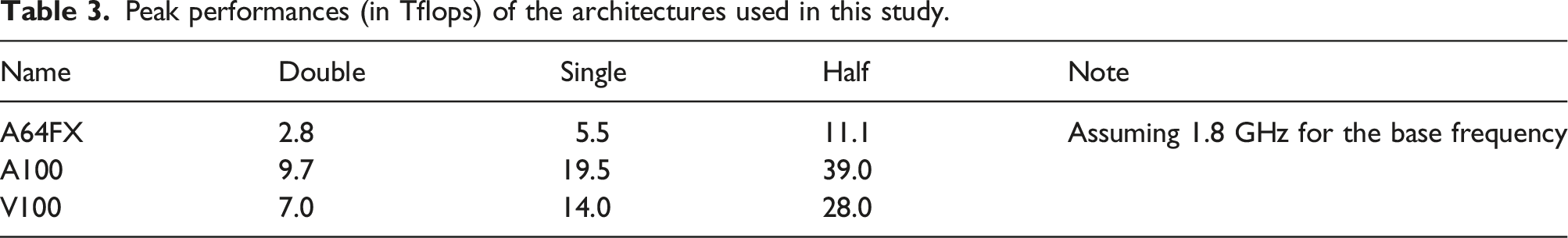
Peak performances (in Tflops) of the architectures used in this study.
5. Test problems
To test our implementation, we simulated the 2D Couette flow and a 3D dam-break test for a more realistic testing. Both problems are widely accepted as test problems for numerical hydrodynamical schemes.
Along the boundaries, we placed “wall” particles that maintain their initial velocity even under accelerations.
5.1. Couette flow
Couette flow defines the flow between two parallel boundaries moving at different velocities. We placed stationary SPH particles in the domains 0 ≤ x < L and 0 ≤ y < L in a Cartesian lattice. Boundary particles mimicking the moving boundary were placed along the vertical boundaries. The upper boundary (y = L) moved at V0 while the lower boundary was stationary. The analytical solution for the x-directional velocity is given by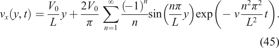
The parameters were set to L = 0.2 and V0 = 6.25 × 10⁻³, and the kinematic viscosity was set to ν = 10−4.
5.2. Dam-break test
The dam-break test models the collapse of a water column. In this test, we adopted the initial setup described in (Kleefsman et al. 2005; Crespo et al. 2011) (see Figure 1). We set a box of dimensions 3.22 × 1 × 1 m (length × width × height). On the right wall of the box, we set a water column of dimensions 1.22 × 1 × 0.55 m (length × width × height). A bump 0.612 × 0.403 × 0.162 m (length × width × height) was set 0.6635 m away from the left wall. Schematics of the side (a) and top (b) views of the dam-break test. All lengths are in meters. Planes H1 and H2 are located 0.992 and 2.638 m away from the left wall.
The water height was varied and measured as H1 and H2 (at distances of 0.992 and 2.638 m away from the left wall, respectively) for validation. The surface heights of the water were observed in a previous laboratory experiment (Kleefsman et al. 2005). The error was computed using equation (40) and the kinematic viscosity was set to ν = 10−6.
6. Results
6.1. Couette flow
Figure 2 shows the evolution of the L2 error of the 2D Couette flow at different precisions with and without scaling and shifting. The L2 error in the standard double precision of the SPH solution without scaling and shifting is also plotted for comparison (the red curve in the upper panel of Figure 2). The L2 error was initially very small Time evolutions of the L2 error in the x-direction velocity of the 2D Couette flow without (top) and with (bottom) scaling and shifting. The blue, green, and red lines are obtained with half-, float-, and double precision, respectively. The number of particles is N = 642. Particle distributions in the 2D Couette flow with N = 642 particles at t = 50T0, 150T0, and 250T0 (T0 = L/V0). The particle colors indicate the x-direction velocity (blue: low, and red: high).
In the naive implementation of the half-precision SPH simulation, the rounding errors cause instability in the solution in the disordered mode, resulting in large density fluctuations. Once large density fluctuations are triggered, the weakly-compressible state worsens because the equation of state is “stiff” (meaning that small density perturbations cause large pressure changes). The consequent fluctuations in the y-direction velocity cause an increase in the L2 error over time. After the scaling and shifting procedure, the contribution of the rounding error was suppressed, and the L2 error converged, and the solution became stabilized (the blue line in the bottom panel of Figure 2).
The lower-precision SPH simulations became disordered earlier than the higher-precision SPH simulations, though the converged error
To examine the effect of spatial resolution on the error, we plotted L2 as a function of number of particles (Figure 4). The error evolutions with different numbers of particles are given in Appendix A. The dashed gray line represents convergence with α = −0.84, which is smaller than the theoretical value (α = −2) predicted by equation (38). L2 error in the x-direction velocity of the 2D Couette flow versus the number of particles in the system. The dashed gray line shows the case for α = −0.84.
From these figures, we can conclude that equation (38) holds; this conclusion implies that equation (43) also holds. Then, equation (43) can be reduced to
Figure 5 shows the wall-clock times of solving one particle per step on each device. The computational performance improved with increasing number of particles because data access became more efficient. The following discussion assumes that the performance saturates when the number of particles exceeds 105. In the Xeon + V100 or EPYC + A100 system, the float- and double precision operations yielded the expected Wall-clock times per particle versus number of particles on each device in the 2D Couette flow test. The blue, green, and red symbols denote the results of half-, float- and double-precision, respectively. Panels (a), (b), (c), and (d) correspond to 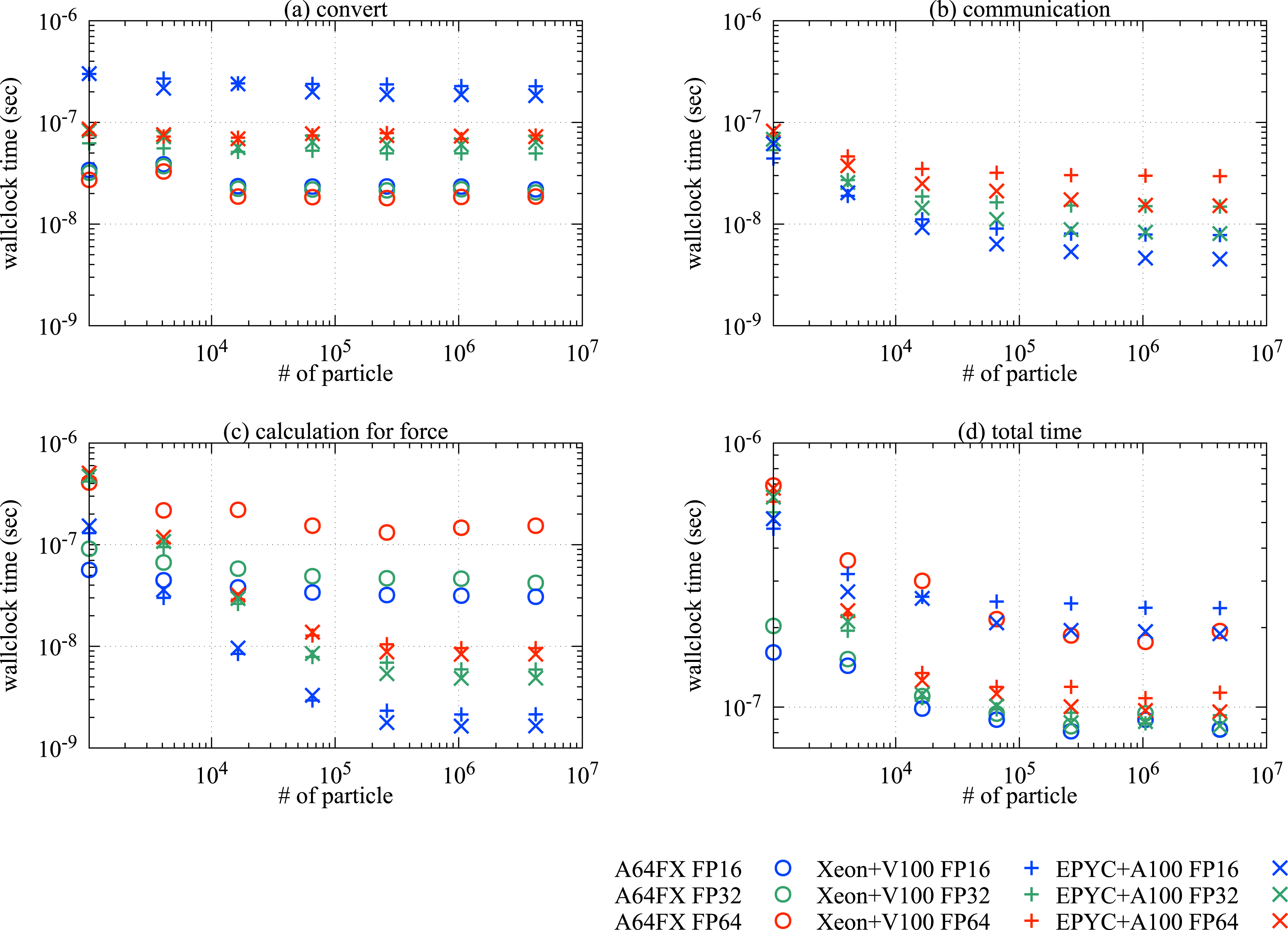
From Figures 5(a) and (c), we can see
Recall that the sum of each of the three wall-clock times
As expected,
These results lead us to conclude that equation (46) does not hold in GPU systems because it does not account for the conversion time, and hence, half-precision is ineffective. However, half-precision is effective in the case of the A64FX system.
6.2. Dam-break test
We first compared the surface heights computed in the 3D dam-break tests at different precisions. All simulations were performed with 106 particles. The evolutions of the fluid heights on planes, H1 and H2, are plotted in Figure 6. Our implementation did not change the quality of the solutions, even at half-precision. Measured heights in the H1 and H2 planes, respectively, in the dam-break test with 106 particles. The blue, green, and red curves show the results of half-, float-, and double-precision, respectively. The gray curve plots the experimental values.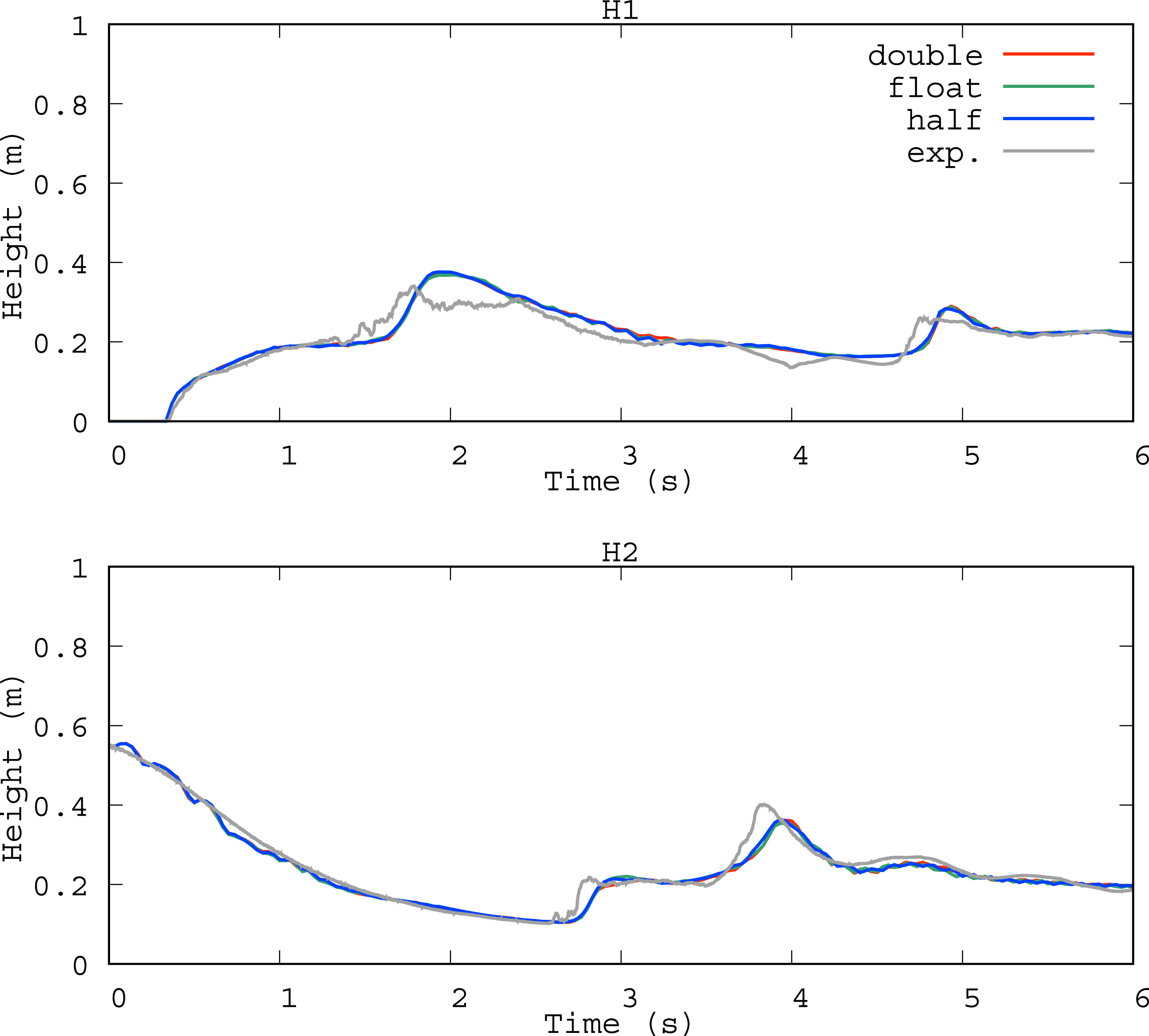
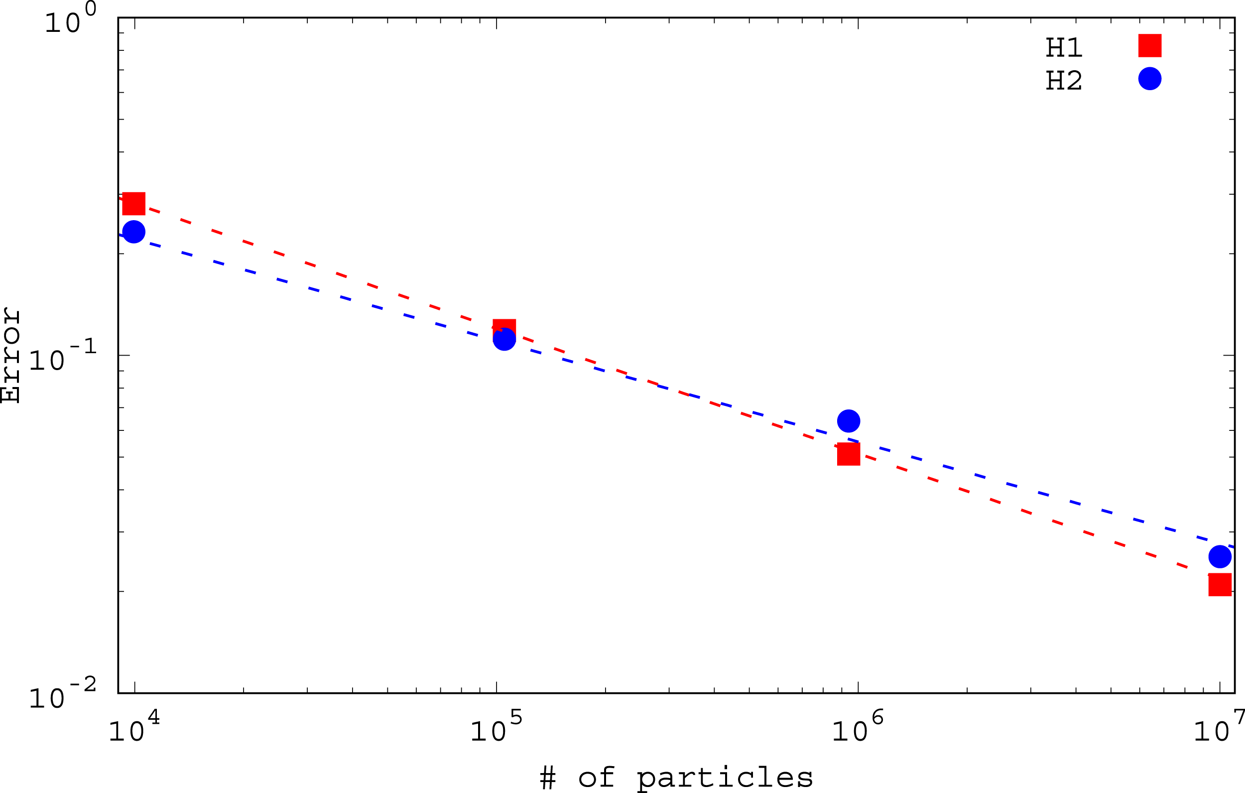
The results of the dam-break test are plotted for different particle numbers in Figure 7. After three runs (double-, float-, and half-precision) with 104, 105, 106, and 107 water particles, the water surface heights approached the experimental values. Figure 8 plots the error convergence versus the number of particles. The convergence equation (38) was satisfied in this problem with α ∼ − 0.34. Convergence of water height in the dam-break test at H1 (top panel) and H2 (bottom panel) for different number of particles: 104 (blue), 105 (green), 106 (red), and 107 (orange). All results were obtained at half precision. The gray curve plots the experimental values. Difference between the numerical and experimental heights, equation (40), versus number of particles at H1 (red squares) and H2 (blue circles) at t = 6. The red and blue lines give α = −0.37 and −0.30 for red and blue lines, respectively.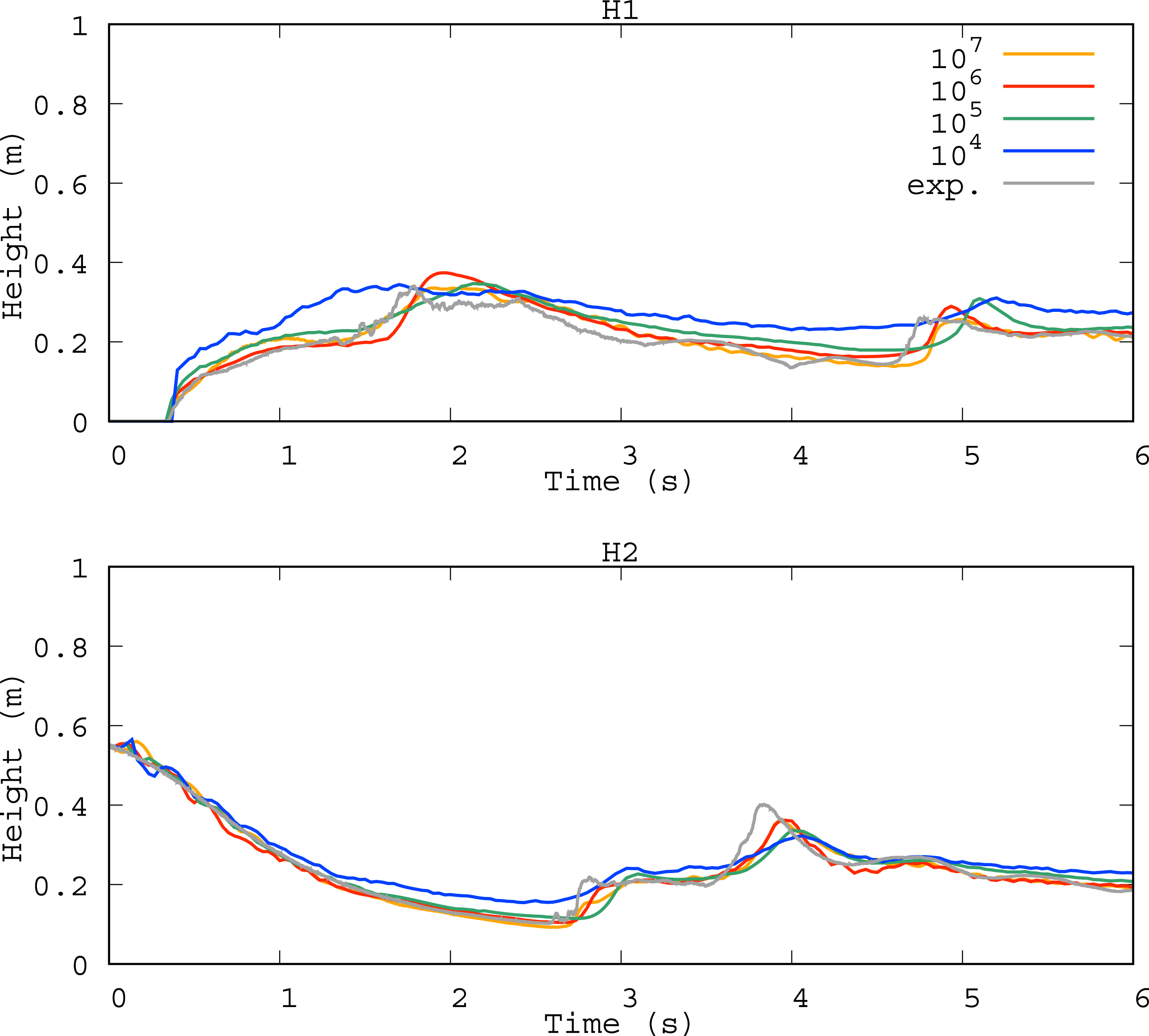
Similarly to the case of 2D Couette flow, equation (43) reduces to equation (46). Therefore, the effectiveness of our proposed implementation relies on the computational performance of low-order precision.
Figure 9 shows the computational performance in the 3D dam-break test. The general trends were similar to those observed in the 2D Couette flow (see Figure 5). In the GPU systems, half-precision can reduce the costs associated with data transfer and force calculation. However, in the Intel Xeon and AMD EPYC systems, the total performance by the half-precision method is degraded because of the high conversion costs. Same results as those in Figure 5, but for the 3D dam-break test.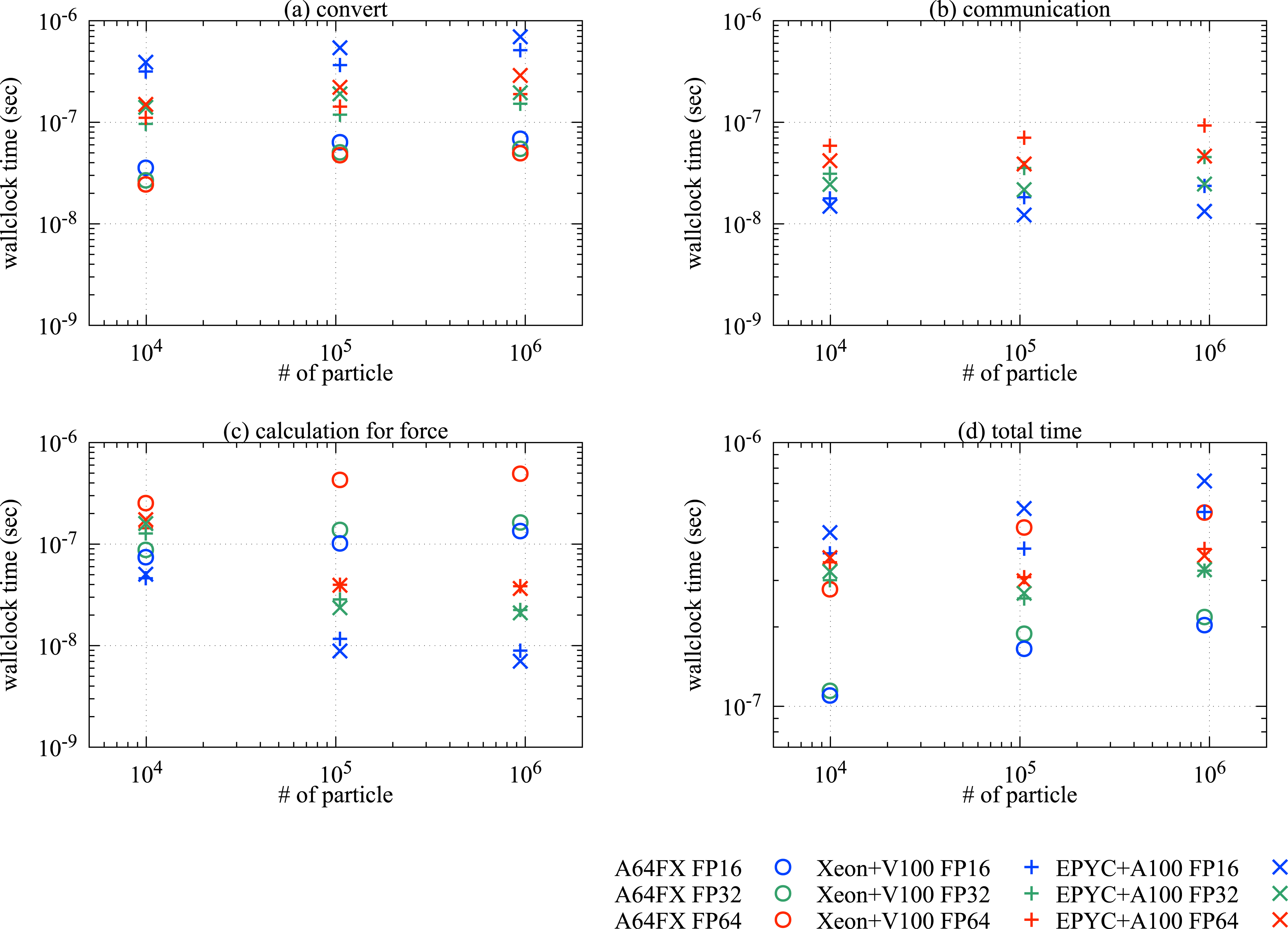
In contrast, in the A64FX system, the conversion cost does not depend on precision. We concluded that in this system, the proposed half-precision SPH method can effectively improve the computational performance of 3D problems without degrading the accuracy.
7. Conclusions
In this study, we examined the effectiveness of half-precision in the SPH method. Half-precision can reduce the cost of arithmetic computations and memory transfers. Thus, it can potentially reduce the time to solution. However, half-precision may worsen the simulation accuracy, which is paramount in scientific computing. Therefore, to verify the potential effectiveness of half-precision, we derived the conditions under which half-precision can reduce the time-to-solution. When solving the test problems in this study, we found that the time-to-solution increased in following the order: half-precision, float-precision, and double-precision. We also checked whether the conditions were satisfied on several modern architectures: Intel Xeon + V100, AMD EPYC + A100, and A64FX. The effectiveness of half-precision depend on the architecture. On the A64FX system, we obtained the expected result

This result is explained as follows: converting double or float precision to half-precision incurs high costs in these systems. Therefore, half-precision fails to reduce the time-to-solution on GPU systems.
The difference in conversion times between A64FX and the other systems arises from the half-precision implementation. Unlike Xeon and EPYC systems, A64FX officially supports half-precision.
In the CPU + GPU systems, the half-precision supported by CUDA was used, but it was not well optimized by the standard compilers for CPUs. This problem can be solved when future CPU compilers support half-precision operations. Moreover, in this work, we conducted the conversion on the CPU side via PCI Express, not on the GPU side, to avoid the slow communication that occurs in double precision. However, GPUs will support coherent memory access in the future; this advancement may greatly reduce the conversion cost by using GPU with fast data transfer capability. Hence, in the next generation of GPU systems, the cost of computing forces will be the only issue that limits overall performance.
Further improvement in conversion and communication costs can be given by the full implementation of the tree method on GPUs. However, because in the particle-based method, particles move dynamically, memory management can be difficult. Although the same problem occurs in the mesh-based method, meshes interact with a fixed number of meshes. Hence, it is beneficial to implement a mesh-based method fully on a GPU to eliminate the conversion and communication costs.
Through scaling and shifting, we maintained the simulation accuracy of half-precision at the same level as that of float/double precision. Without these procedures, simulations with half-precision can violate the accuracy requirements.
Our method is applicable to other AI processors, such as the AMD Instinct MI or Preferred Networks MN-3. Our implementation on these processors will be discussed in future work.
Another possible future work is the use of an integer type. Converting the exponent bit to a fraction bit can enhance the accuracy, but it leads to the risks of overflow error.
Footnotes
Acknowledgements
We thank two anonymous referees for carefully reading our manuscript and providing helpful comments. This paper is based on results obtained from a project, JPNP16007, commissioned by the New Energy and Industrial Technology Development Organization (NEDO). We used the computational resources of FUGAKU at the RIKEN Center for Computational Science (project id: ra000010). This study was supported by the Earth Simulator project of the Japan Agency for Marine-Earth Science and Technology, and the supercomputer FUGAKU provided by RIKEN through the HCPI System Research Project (Project ID:hp210054), a Grant-in-Aid for Scientific Research (JP18K03815) from the Japan Society for the Promotion of Science.
Declaration of conflicting interests
The author(s) declared no potential conflicts of interest with respect to the research, authorship, and/or publication of this article.
Funding
The author(s) disclosed receipt of the following financial support for the research, authorship, and/or publication of this article: This work was supported by the New Energy and Industrial Technology Development Organization (JPNP16007).
Appendix
Author biographies