
Abstract
We present a new parallel spectral element solver, FNPF-SEM, for simulating linear and fully nonlinear potential-flow-based water waves and their interactions with offshore structures. The tool is designed as a general-purpose wave model for offshore engineering applications. Built on the open-source Firedrake framework, the new FNPF-SEM model is a computational tool capable of capturing both linear and nonlinear wave phenomena with high accuracy and efficiency, supporting high-order (spectral) finite elements. Additionally, Firedrake provides native support for MPI-based parallelism, enabling efficient multi-CPU distributed computations for large-scale simulations. We demonstrate the capabilities of the high-order model through h- and p-convergence studies, and weak and strong scaling tests. Verification is performed against analytical and numerical solutions and verified against experimental data, including nonlinear high-order harmonic generation and wave interactions with a cylinder and a breakwater. The new FNPF-SEM model offers a numerical framework for simulating wave propagation and wave-structure interactions, with the following key features: (i) the ability to represent complex geometries through flexible, unstructured finite element meshes; (ii) reduced numerical diffusion and dispersion by using high-order polynomial expansions; and (iii) scalability to full- and large-scale simulations over long time periods through a parallel implementation.
Keywords
1. Introduction
Simulating the dynamics of water waves remains a significant challenge in computational fluid dynamics (CFD), especially when complex geometries are present in the flow domain and marine or offshore structures are included. However, despite the challenge, accurate modeling of wave propagation and interactions with bathymetry and structures is essential for marine and offshore engineering applications. For example, estimating how the local wave climate and the resulting wave-induced forces impact offshore structures such as large offshore wind turbines Bailey et al. (2015), wave energy devices, and breakwaters. Other cases include metocean studies such as assessments of ocean conditions, Bitner-Gregersen (2015). Many offshore engineering applications must model nonlinear water waves over large regions and over long time scales, requiring effective parallel implementations of these wave models to accurately and efficiently simulate real-world scenarios within acceptable computational times.
Physical accuracy is typically associated with the chosen mathematical model and its representation of the physics. High-fidelity simulations can be based on the Navier-Stokes equations as a model for all fluid flows. However, when solved numerically, these equations come with high computational requirements. For offshore engineering applications, a broad range of free-surface flows can be approximated by fully nonlinear potential flow (FNPF), assuming the fluid is incompressible, inviscid, and irrotational, Dean and Dalrymple (1991). Moreover, if the wave steepness is small, the linear potential flow (LPF) equations are applicable, i.e., a small-amplitude approximation, which reduces the problem’s complexity. One desirable feature of the FNPF formulation is its ability to simulate both offshore and nearshore environments, as wave interactions with the bathymetry are accurately represented, Bihs et al. (2020). When the simulated problem satisfies the assumptions of FNPF theory, a performance improvement of at least two orders of magnitude can be achieved while achieving an accuracy comparable to the full CFD simulations, as shown in Ransley et al. (2019). If the problem adheres further to the assumptions of LPF theory, additional orders of magnitude in computational efficiency can be realized.
Numerically accurate and efficient solutions to FNPF and LPF formulations have been a major research topic for decades; see, e.g., the report by Evans and Newman (1987) from the 1980s and the references herein and the review by Thomas and Dwarakish (2015). Traditionally, the boundary integral method has been popular for wave modeling. To highlight a few of the well-known and recent boundary element-based models (including the traditional low-order boundary element method, the quadratic boundary element method, and the high-order boundary element method), see Liu et al. (2001); Xue et al. (2001); Lee and Newman (2006); Yan and Liu (2011); Harris et al. (2022); Kurnia and Ducrozet (2023); Seixas De Medeiros et al. (2024). Another option are high-order spectral methods, which are very efficient when modeling nonlinear wave propagation and submerged wave-structure interactions, Dommermuth and Yue (1987); Liu et al. (1992); Christiansen et al. (2013); Melander and Engsig-Karup (2024). The FNPF and LPF equations have also been solved using finite difference schemes, Bingham and Zhang (2007); Engsig-Karup et al. (2009); Ducrozet et al. (2010); Amini-Afshar and Bingham (2017, 2018); Bihs et al. (2020), and with harmonic polynomials, Shao and Faltinsen (2014); Tong et al. (2024). Employing the classical second-order accurate finite element method, we have the work by Wu and Eatock Taylor (1994) and many more, e.g., see Le Roux et al. (2000); Wu and Hu (2004); Ma and Yan (2009).
Spectral element methods (SEMs), initially introduced by Patera (1984), combine key advantages of both spectral (polynomial) and finite element methods. SEMs allow for two distinct convergence strategies: (i) h-convergence, where the mesh is refined while maintaining a fixed polynomial order, resulting in algebraic convergence; and (ii) p-convergence, where the mesh is held fixed while increasing the polynomial order of the basis functions, typically leading to spectral (exponential) convergence. The hybrid approach provides efficient, highly accurate numerical solutions by using piecewise polynomial basis functions of arbitrary order with spectral accuracy. Moreover, the SEM can handle complex geometries common in engineering applications because it uses unstructured mesh tessellations. This combination of high accuracy and geometrical flexibility addresses the limitations of traditional numerical approaches, e.g., the difficulty in modeling complex geometry (finite difference) and/or high dispersive and diffusive errors (low-order finite and boundary elements). For further details and applications of the SEM, see the review by Xu et al. (2018) and the textbook by Karniadakis and Sherwin (2005).
Many open-source finite element frameworks that allow for high-order basis functions and parallel computing have been developed over the years. For example, the spectral/hp element framework Nektar++, Cantwell et al. (2015), the arbitrary high-order finite element framework MFEM, Anderson et al. (2021), the deal.II finite element framework, Arndt et al. (2021), or libParanumal, Chalmers et al. (2022). Another computational framework that supports high-order basis functions is Firedrake, Ham et al. (2023). Firedrake is an open-source framework that automates the solution of partial differential equations using finite elements. One of Firedrake’s main features is the unified form language, Alnæs et al. (2014), which allows the symbolic expression of, e.g., weak variational formulations. Moreover, Firedrake runs with Python, uses state-of-the-art PETSc solvers, Balay et al. (1997, 2024), and supports both structured and unstructured meshes, including the most common element types and finite element spaces. Lastly, Firedrake supports fully parallel computation via MPI and can run on large many-core systems. In the recent decade, the Firedrake project has established itself as a robust open-source platform for implementing advanced numerical models.
At DTU, SEM-based FNPF models for simulating free surface water waves have been under active development for more than a decade. This effort began with the work of Engsig-Karup (2006); Engsig-Karup et al. (2006) and later Engsig-Karup et al. (2016), where a solution was proposed to the intrinsic mesh-induced instability associated with finite element discretizations of free surface flows, as previously identified in Robertson and Sherwin (1999). The SEM implementations at DTU are based primarily on the FNPF formulations, Engsig-Karup et al. (2016); Engsig-Karup and Eskilsson (2019); Engsig-Karup et al. (2019); Engsig-Karup and Laskowski (2021); Visbech et al. (2026c), and the LPF approximations, Visbech et al. (2024a,b). This FNPF-SEM approach offers a numerical method that can handle complex geometries and accurately simulate over long time periods using a high-order polynomial basis. The methodology has been extended to encompass the full incompressible Navier-Stokes equations with a free surface in Melander et al. (2024). Achieving low dispersive and diffusive numerical errors arising from the numerical discretization procedure is a key aspect of long-time wave simulations. High-order discretization methods, such as SEM and others, are much more efficient than low-order methods, such as classical p = 1 finite elements, Kreiss and Oliger (1972); Willberg et al. (2012). In addition, Eskilsson et al. (2025) presented a high-performance implementation of an FNPF-based water wave solver using Nektar++. The current capabilities of these FNPF-based SEM models are comparable in functionality, benefiting significantly from the robust, scalable features of modern open-source computational frameworks. Moreover, efficient water wave solutions to the Benney-Luke-type equations, derived using variational principles, are also available via Firedrake, Bokhove and Kalogirou (2016). Furthermore, the Thetis project, an unstructured-grid coastal ocean model, was built using the Firedrake framework, Kärnä et al. (2018). Very recently, steady-state solutions to the incompressible Navier-Stokes equations were presented by Minniti et al. (2025) through a Firedrake implementation.
1.1. Paper contribution
The main aim is to demonstrate the correctness of a new parallel implementation of the aforementioned DTU-based SEM models for solving FNPF and LPF wave problems. The parallel code is implemented in Firedrake, enabling efficient parallel solution of the FNPF equations for large- and full-scale wave problems over long time horizons, ultimately for use in offshore engineering applications. The paper verifies the numerical implementation, referred to as FNPF-SEM, through h- and p-convergence studies and the parallel setup through strong and weak scaling tests. Moreover, the entire model is further verified and validated across various test cases for FNPF and LPF wave propagation and wave-structure interactions.
1.2. Outline of paper
Following the introduction in Section 1, the paper proceeds with the mathematical model in Section 2, which describes the computational domain, its boundaries, and the governing equations. Subsequently, Section 3 outlines the numerical discretization methods, highlighting the chosen spatial and temporal discretizations and key aspects such as wave initialization, generation, and absorption. The results are presented in Section 4, which includes both numerical verification studies (including convergence and scaling analyses) and cases of linear and nonlinear wave propagation and wave–structure interactions. Finally, the paper concludes with a summary of the main findings in Section 5. An appendix containing supplementary material (additional convergence studies, mesh layouts, and simulation results) is included at the back.
2. Mathematical model
Considering a fluid domain, Conceptual schematic of the fluid domain, Ω, and its boundaries in the xz-plane.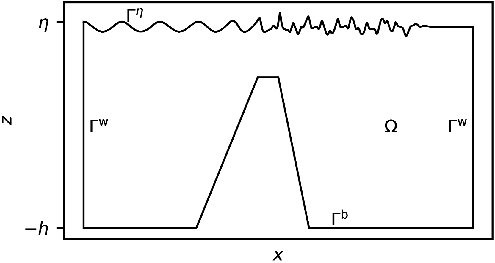
2.1. Governing equations
Assuming potential flow, i.e., an incompressible, irrotational, and inviscid fluid, the gradient of a scalar velocity potential,


Here

3. Numerical discretization
We adopt a classical method of lines approach to the governing equations. The spatial and temporal discretizations are discussed below individually. As stated earlier, the mathematical model is implemented in Firedrake, Ham et al. (2023). Firedrake is an open-source computational framework for solving partial differential equations using the finite element method. It provides a high-level interface based on the unified form language, Alnæs et al. (2014), allowing users to express weak variational formulations in a compact, readable form. At the backend, Firedrake automates the generation of optimized C code and supports efficient parallel execution via MPI, making it well-suited for large-scale simulations. Built on PETSc, Balay et al. (2024), it includes state-of-the-art solvers and supports a wide range of element types and mesh structures, including high-order spectral elements on both structured and unstructured meshes.
3.1. Spatial discretization
We perform a discrete tesselation of the spatial domain, Ω, and boundary, Γ
η
, using non-overlapping finite elements as

3.1.1. Weak variational formulations
Next, we state the weak forms of (1) and (2) through (3), respectively. The linearized forms in (4) are omitted for brevity. The linear variational problem for the Laplace problem is to find

For the two free surface conditions, we define a nonlinear variational problem to find

3.1.2. Initial meshes, extrusion, and mesh updating
Firedrake has native support for extruded meshes, McRae et al. (2016); Bercea et al. (2016). The mesh construction for this model proceeds in three steps: First, a triangular mesh for the free surface, Point distribution (indicated by different colors) for a finite FNPF wave tank distributed over N
c
= 5 cores on a mesh with (N
x
, N
y
, N
z
) = (20, 4, 4) elements of order p = 5.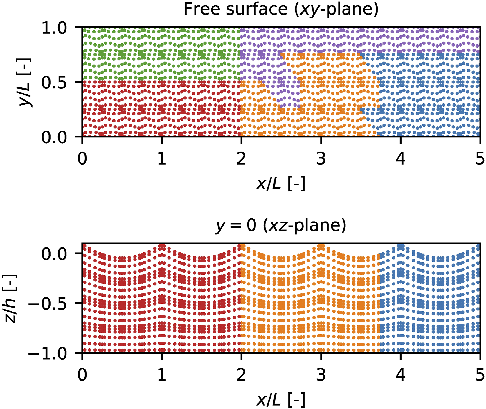
We want to move information and data (when running in parallel) between the free surface mesh,
3.2. Temporal discretization and modal filtering
Time integration is performed using a standard explicit 4th-order, 4-stage, Runge-Kutta scheme (ERK4). The time step size, Δt, is kept constant throughout the simulation and is computed based on a Courant-Friedrichs-Lewy (CFL) condition:
Some form of stabilization is typically required to accurately model strongly nonlinear wave phenomena. In Engsig-Karup et al. (2016), the instability issue initially highlighted by Robertson and Sherwin (1999) was addressed using structured elements aligned in the vertical direction. This was coupled with an over-integration (collocation) approach for the nonlinear free surface terms, Kirby and Karniadakis (2003), and a mild modal (spectral) filter applied to the free surface quantities, Hesthaven and Kirby (2008). In Firedrake, the integration order of individual integral terms can be explicitly specified, facilitating the over-integration strategy suitable for reducing aliasing instabilities of nonlinear wave propagation, Engsig-Karup et al. (2016). A modal filter was implemented within this framework by developing a custom
Then, the filtered solution can be mapped back to nodal space

This filtering approach can be applied to any free surface quantity, e.g., η, ϕ η , or w η , as needed for nonlinear waves.
3.3. Wave initialization, generation, and absorption
For periodic wave tank simulations, the model is initialized with η and ϕ
η
, either from the linear wave theory in the LPF setting or from an accurate stream function solution in the FNPF setup, Fenton (1988). Linear (small-amplitude) waves can be fully characterized by the non-dimensional wave number, kh, given a specified wavelength, L, or water depth, h. In contrast, nonlinear (finite-amplitude) stream function waves also require the specification of a relative wave steepness, ɛ/ɛmax, to quantify their nonlinearity. Here, ɛ = H/L denotes the wave steepness based on the wave height H, and ɛmax is the maximum steepness attainable before wave breaking for a given wave, Fenton (1990). The initial conditions are set to zero for simulations in numerical wave tanks of finite size. Wave generation and absorption are handled using classical relaxation zones, Larsen and Dancy (1983), of 2-3 wavelengths in size. The wave fields, η and ϕ
η
, are then modified at each time step as a post-processing operation as
3.4. Entire computational workflow
To support the understanding of how the entire computational workflow is outlined, a step-by-step procedure is shown below:
4. Results
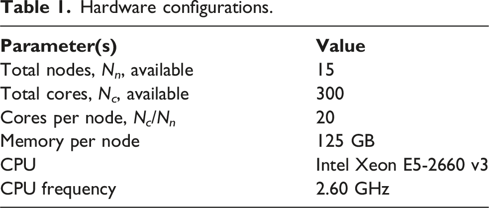
Hardware configurations.
As for the numerical solver strategies, we solve the Laplace problem in (1) following Rathgeber et al. (2016) by using a CG solver with the HYPRE BoomerAMG algebraic multigrid preconditioner, Hestenes and Stiefel (1952); Falgout et al. (2006), using a relative and absolute tolerance of 10−6 and 10−15, respectively. For the evaluation of the two nonlinear free surface conditions in (2) and (3), we employ the default solver using a GMRES strategy with an ILU as preconditioner and a relative and absolute tolerance of 10−5 and 10−15, respectively. For this study, this leads to an efficient solver strategy for the cases considered, cf. the analysis of iterative solver efficiency for FNPF modeling reported in Engsig-Karup (2014).
4.1. Model verification
During model verification, various timings will be presented. Those timings are an average for the number of cores, N c , used in the test. When using N c ≤ 20, a complete node is allocated to the run.
4.1.1. Convergence h/p-studies
Investigating and confirming the expected convergence rates of the proposed model constitutes the first step in the verification process. For this, we perform h- and p-convergence studies; that is, mesh refinement under a fixed polynomial order of the basis functions, and an increase in the polynomial order on fixed meshes, respectively. For the analysis, a periodic domain is considered, featuring nonlinear waves for all combinations of kh = {1, 3, 6} and ɛ/ɛmax = {10%, 50%, 90%}. The error is evaluated in the ∞-norm of the vertical free surface velocity,
The results of the h-refinement convergence study are presented in Figure 3, using basis functions of order p = {1, 2, 3, 4, 5}. The parameter hmax denotes the maximum length of the element in the computational mesh. Due to the gradient recovery of w from ϕ, it is well known that an order of algebraic convergence is typically lost, Engsig-Karup et al. (2016), leading to an expected convergence rate of Convergence study for h-refinement for nonlinear waves in all combinations between kh = {1, 3, 6} and ɛ/ɛmax = {10%, 50%, 90%}.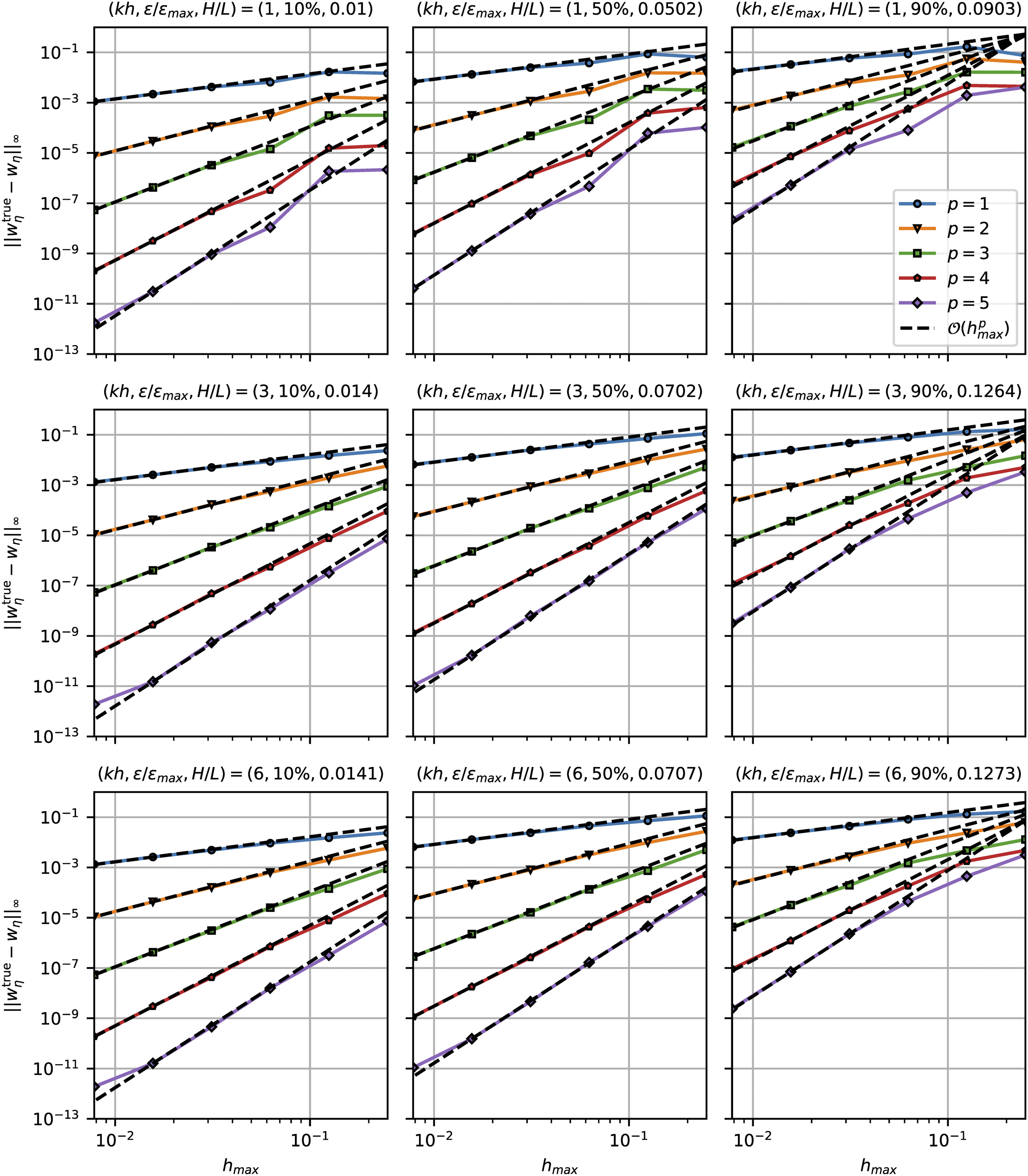
The p-convergence study is presented in Appendix C, in Figure 19, where spectral, i.e., exponential, convergence is observed. The test is conducted on six different meshes with increasing resolution. Specifically, Mesh 1 has hmax = 0.25, Mesh 2 has hmax = 0.125, Mesh 3 has hmax = 0.0625, etc. As observed previously, increasing nonlinearity makes the problem more challenging, requiring higher resolution to achieve comparable accuracy.
4.1.2. Performance profiling
It is well established that solving the Laplace problem constitutes the primary computational bottleneck in both LPF and FNPF wave models. Distributing the finite element domain across multiple cores inevitably affects performance. To this end, we profile the three most computationally intensive routines involved in time integration: (1) LaplaceSolve, which includes imposing boundary conditions, solving the linear system of equations, and performing gradient recovery (
Performance profiling meshes with fixed N z = 4 and p = 4.
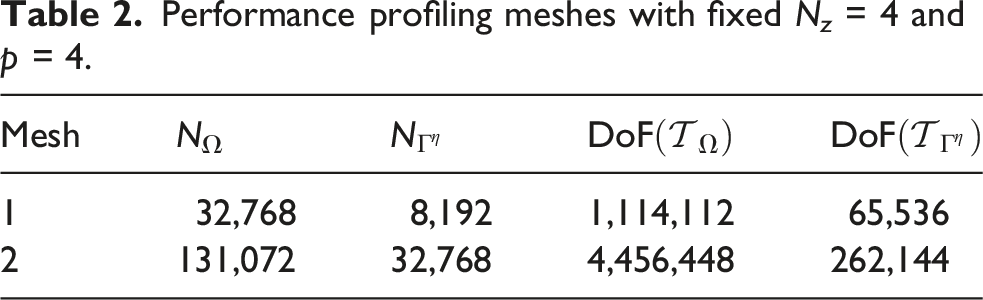
Figure 4 presents the core-averaged timing for each time stage across the three routines. A substantial reduction in time per stage is observed; the increase is from N
c
= 1 to approximately N
c
= 20. Beyond this point, only the LaplaceSolve routine continues to benefit from further parallelization, while EvaluateRHS and LaplaceUpdate begin exhibiting constant runtimes. Moving to a finer mesh (Mesh 2) increases the computational time for both LaplaceSolve and EvaluateRHS, as expected. In contrast, LaplaceUpdate remains largely unaffected by mesh resolution, suggesting that its performance is dominated by communication overhead. The stagnation in EvaluateRHS scalability is attributed to the relatively small size of the free surface mesh, which limits the parallel efficiency of this part. However, the overall solver remains scalable as long as LaplaceSolve is the dominant cost factor. Moreover, comparing the results of Mesh 1 and 2 shows that increasing the problem size enables scalable behavior across more cores, as LaplaceSolve is the dominant cost factor for longer runs. Timings for routines in the FNPF model for Mesh 1 (blue) and Mesh 2 (red), using a polynomial order p = 4.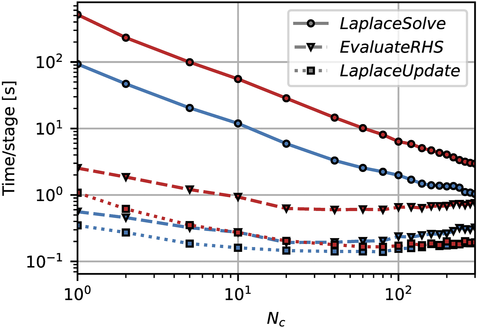
Figure 5 shows the relative percentage distribution of the total run time across the three routines. At low core counts (e.g., N
c
≤ 5), LaplaceSolve dominates the computational cost. However, as N
c
increases, its relative share decreases because the remaining routines incur a constant cost. For larger problems (as in Mesh 2), this imbalance is somewhat mitigated. Potential optimizations include reducing the core count assigned to the free-surface evaluation, as done in Eskilsson et al. (2025), or implementing more efficient iterative solvers for the nonlinear free-surface problem. These optimizations are left for future work. Percentage distribution of computational cost across routines for Mesh 1 (blue) and Mesh 2 (red), using p = 4.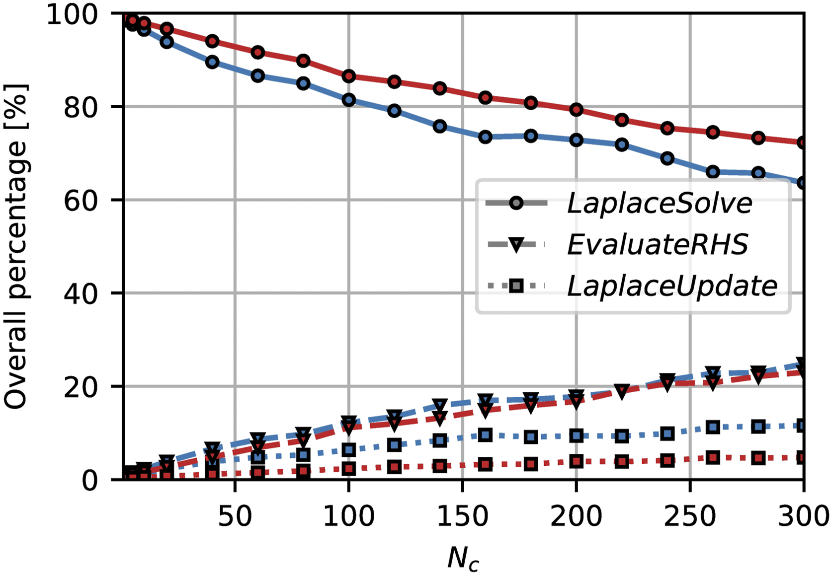
Based on this code performance profiling, it is confirmed that the Laplace solver is the primary computational bottleneck. Consequently, the following strong- and weak-scaling analyses focus exclusively on this part of the code. Moreover, the convergent behavior showcased in the previous section has been confirmed on multicore hardware setups as well; however, it is omitted for conciseness.
4.1.3. Parallel performance: Strong scaling
Strong scaling meshes with N z = 4.
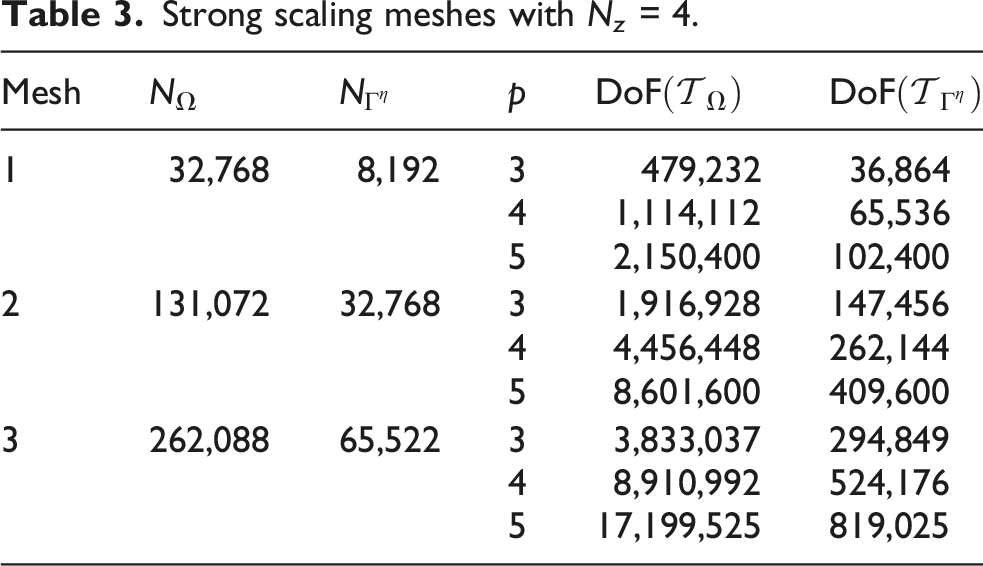
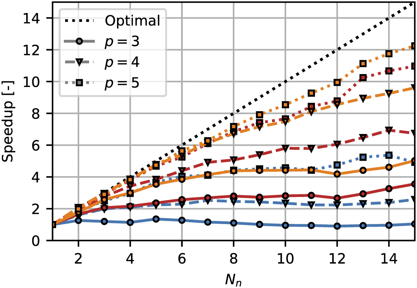
Figure 6 shows the strong scaling efficiency using (7) for the three meshes. As expected, both increased mesh refinement and higher polynomial order improve the model’s parallel efficiency. This reflects better utilization of computational resources for larger problem sizes. The corresponding speedup curves are presented in Figure 7, alongside an ideal speedup line. The results indicate that the model approaches optimal speedup behavior as the problem size increases. For smaller problems, however, speedup plateaus early, revealing limitations in parallel efficiency due to insufficient workload per core. Strong scaling efficiency test. Mesh 1 (blue), Mesh 2 (red), and Mesh 3 (orange) with polynomial orders p = {3, 4, 5}. Speedup (compared to N
n
= 1 as baseline) for the strong scaling test. Mesh 1 (blue), Mesh 2 (red), and Mesh 3 (orange) with polynomial orders p = {3, 4, 5}.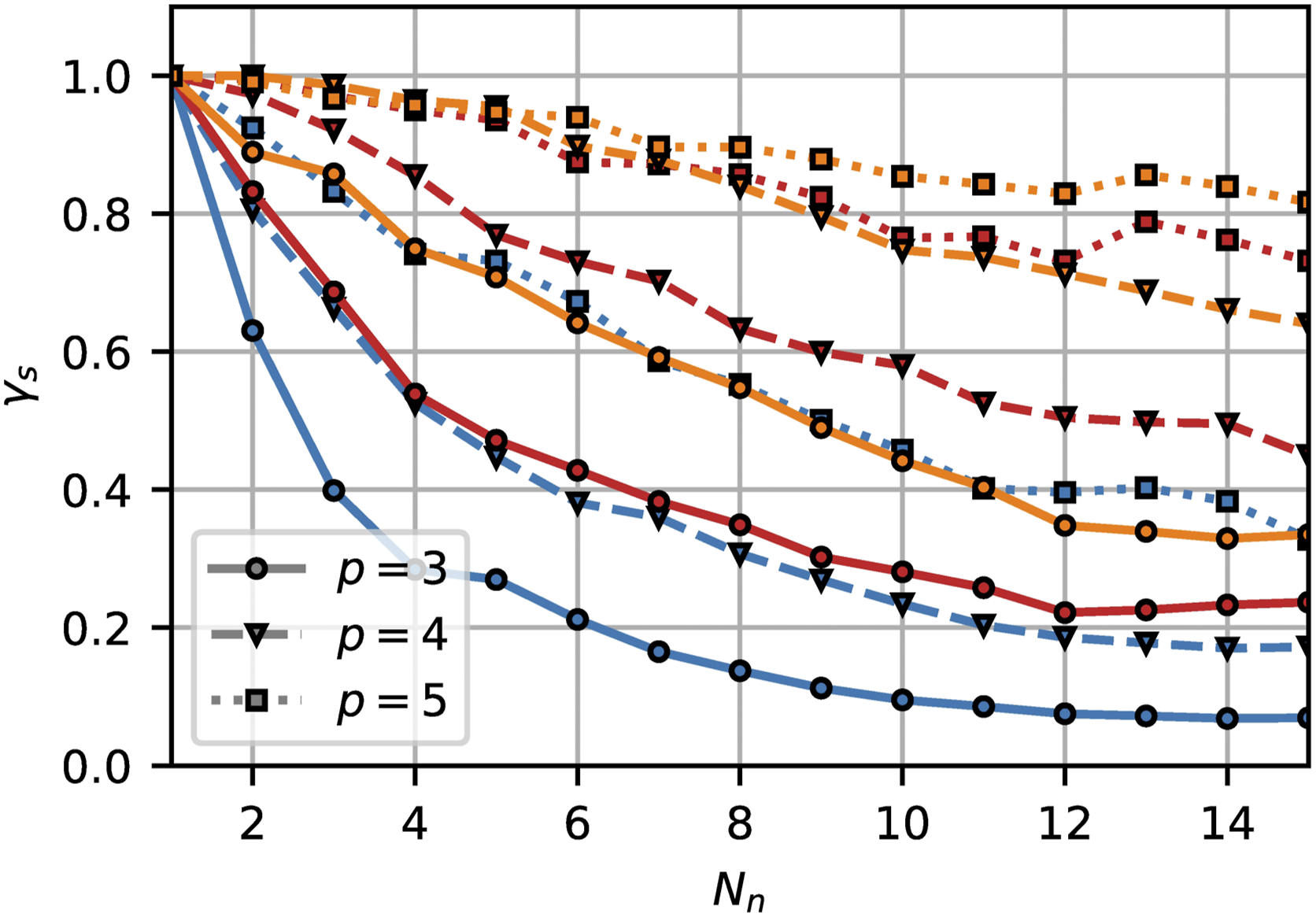
4.1.4. Parallel performance: Weak scaling
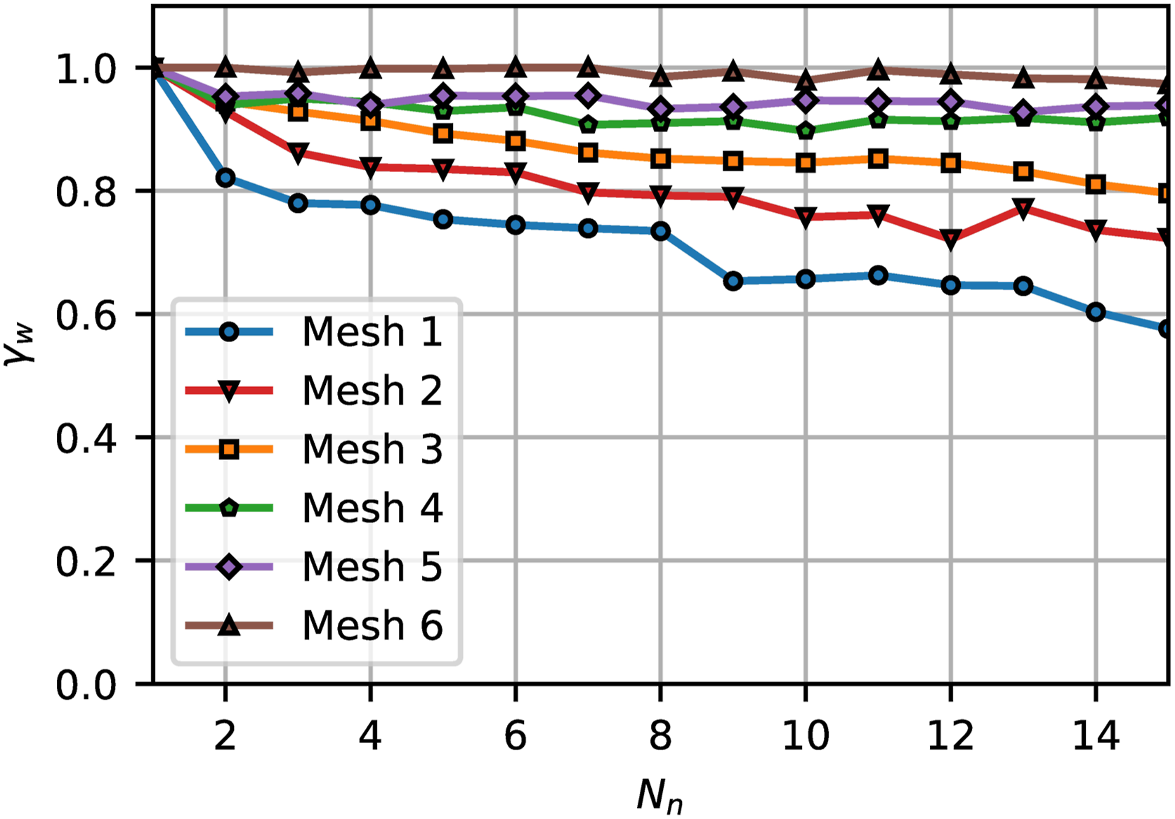
Weak scaling meshes with N y = N z = 4 and polynomial order p = 5. All reported quantities are per core, N c .
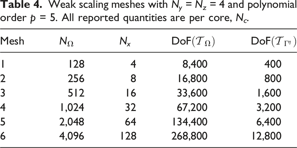
Figure 8 presents the run times for the various mesh configurations. As expected, increasing resolution increases run time. However, more importantly, the runtime remains nearly constant as the number of cores increases, confirming the model’s weak scaling behavior. This trend is further analyzed in Figure 9, which shows the weak scaling efficiency using (8). The results indicate that higher mesh resolutions lead to improved parallel efficiency, as the computational workload per core becomes more substantial relative to communication overhead. Weak scaling timings on six meshes with p = 5. Weak scaling efficiency on six meshes with p = 5.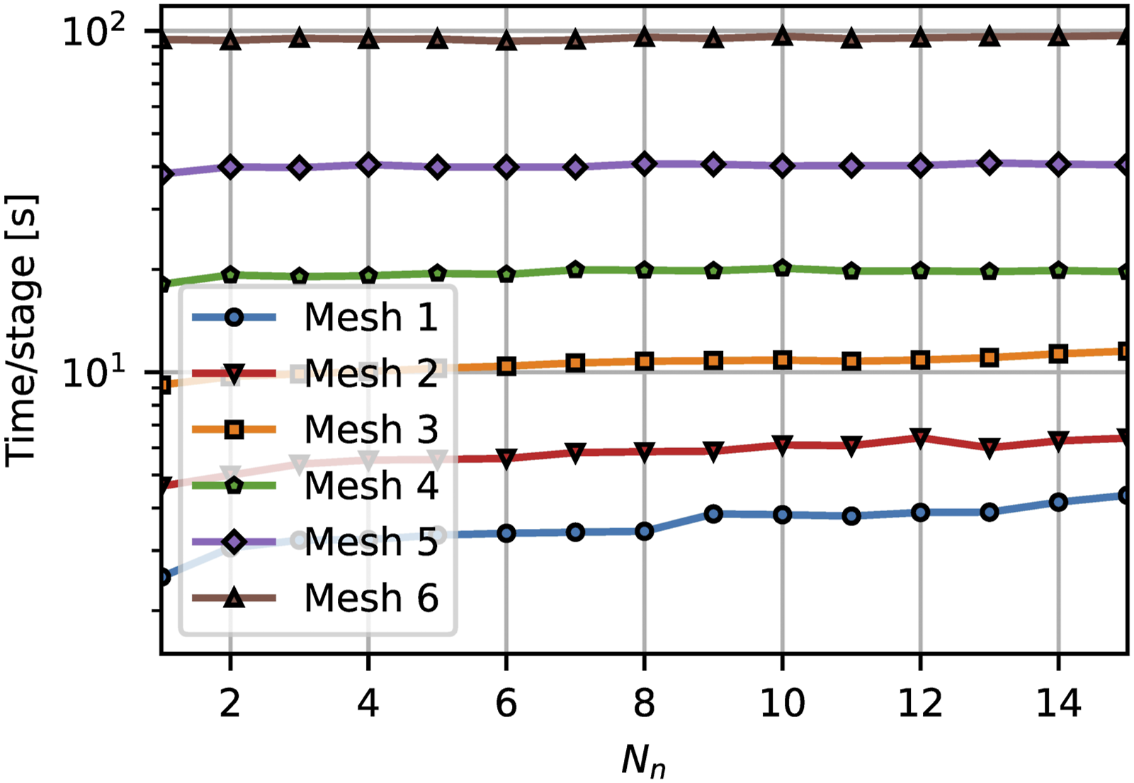
4.2. Simulations
For all the following cases, the simulations are run on a full node (N c = 20 cores).
4.2.1. Generation of high-order wave harmonics over a submerged bar
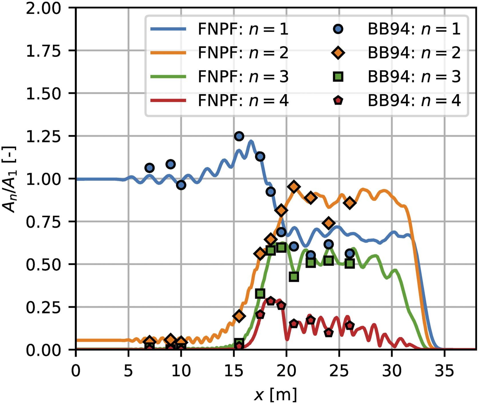
First, we consider the classical bar test, which can be compared with the physical experimental laboratory data by Beji and Battjes (1994), denoted as BB94 in the following. Note that this is a wave flume test, thus two-dimensional; however, we extend the domain in the y-direction to match our three-dimensional model. Mildly nonlinear waves are generated and propagated over a submerged bar, which generates high-order wave harmonics due to nonlinear shoaling effects (steepening and shortening of the waves). The domain is sketched out conceptually in Figure 1, where the specifications of the domain are: Generation zone (0 ≤ x ≤ 8), target zone with the submerged bar (8 ≤ x ≤ 30), and absorption zone (30 ≤ x ≤ 38). The width of the domain is 0 ≤ y ≤ 1. All units are [m]. The depths before and after the bar are h = 0.4 [m] and h = 0.1 [m] above the bar. The incline before and decline after the bar are 1:20 and 1:10, respectively. The input wave characteristics are set as kh = 0.6725 [-] and ɛ/ɛmax ≈ 7% given a wave period of T = 2.018 [s]. For the simulation, we used a free-surface mesh of 7600 elements, extruded with N z = 4 elements in the vertical direction, yielding 22,800 prismatic elements to represent Ω. Ultimately, this yields problem sizes of 810,693 DoF and 62,361 DoF for Ω and Γ η , respectively, when using basis functions of order p = 4. The simulation is run for 25 wave periods.
A contour plot of the free surface elevation, η, at the final time is shown in Figure 10. Here, the high-order harmonic is observed to occur when the wave reaches the submerged bar. In addition, a harmonic decomposition of the wave signal is carried out and presented in Figure 11. The harmonic analysis is performed by fitting the time series, both experimental and numerical, using a least-squares approach to a sum of sinusoidal functions with argument 2πf
n
t, where f
n
= n/T and n = {1, …, 4}. The figure illustrates how waves with dominant first-order components, along with minor second-order contributions, propagate toward the bar. Over and beyond the bar, second-order components begin to dominate the wave dynamics, with contributions from the first, third, and fourth harmonics. Finally, in the absorption zone, all wave energy is dissipated. The comparison between the numerical solution (FNPF) and the experimental data (BB94) shows good visual agreement. Contour of the free surface elevation at t = 25T. Harmonic analysis of the numerical simulation (FNPF) and experimental data (BB94) for the most dominant harmonic modes in the bar test. A1 = H/2 = 0.01 [m].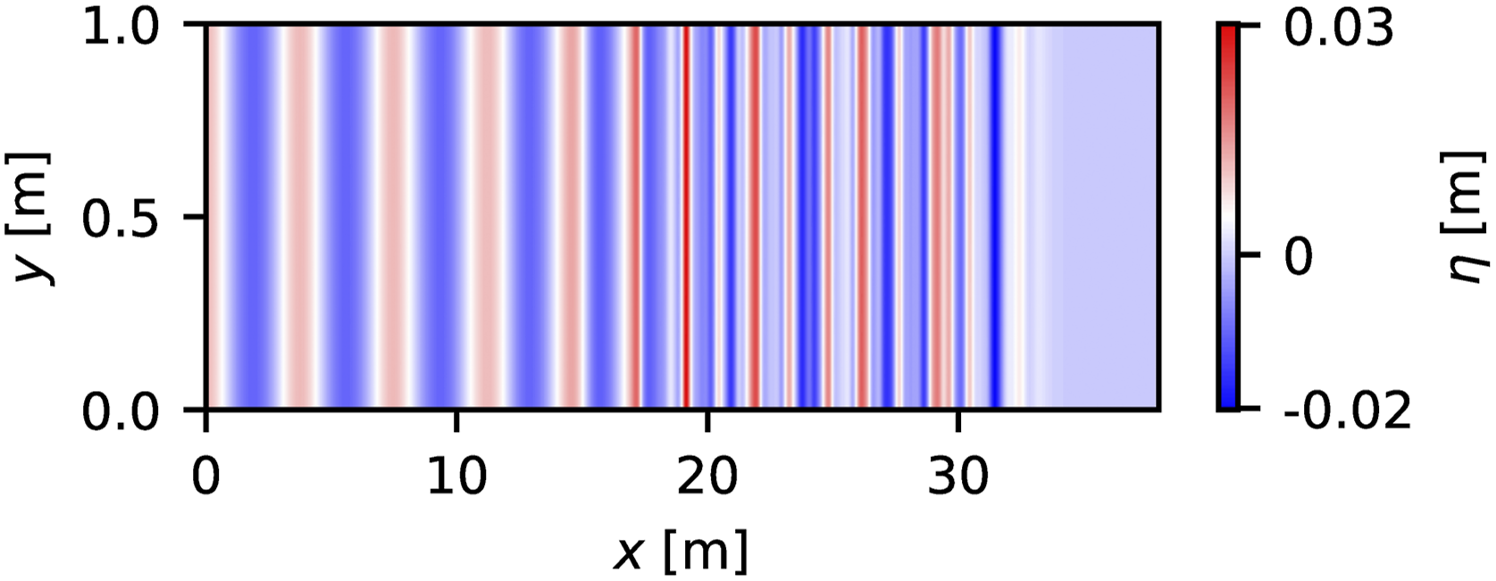
4.2.2. Linear and nonlinear interactions with a vertical cylinder
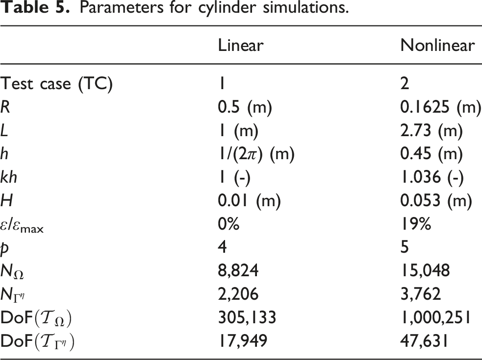
Parameters for cylinder simulations.
The results from both simulations are shown in Figure 12, presented as the non-dimensional maximum free-surface elevation at the cylinder boundary, η
m
/(2H). Here, η
m
is Maximum non-dimensional free surface elevation on the cylinder, η
m
/(2H), for the two simulations comparing numerical, experimental, and analytical solutions.
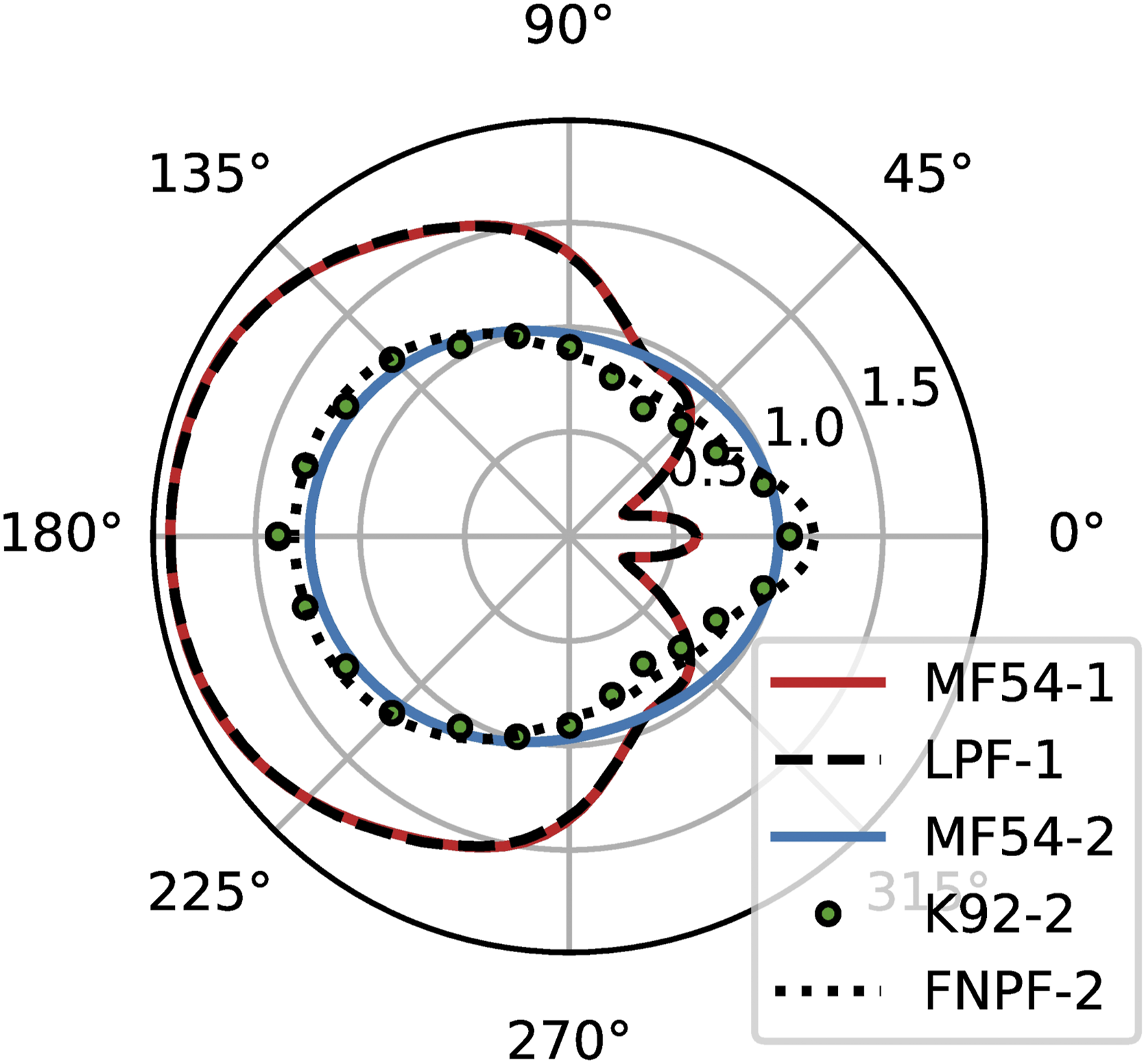
For the linear test case (TC 1), the numerical results, denoted LPF-1, are compared with the analytical predictions of linear diffraction theory by MacCamy and Fuchs (1954), denoted MF54-1. For the nonlinear test case (TC 2), the numerical results of the FNPF simulation, denoted FNPF-2, are compared with the digitized experimental data of Kriebel (1992), denoted K92-2, which were digitized for comparison. We also include equivalent linear results for this configuration, denoted MF54-2.
Figure 12 shows good agreement between the numerical and analytical results for the linear case (LPF-1 vs MF54-1), particularly in the region downstream of the cylinder. For the nonlinear test case, the numerical solution (FNPF-2) aligns well with the experimental data (K92-2), consistent with previous results reported in the literature (e.g., see Ducrozet et al. (2010)). Notably, nonlinear effects (compared to MF54-2) manifest as increased run-up at 0° and 180°, and a reduced run-up at intermediate angles, around 45° and 315°.
4.2.3. Wave interactions with a V-shaped breakwater
As a final verification test case, we consider wave interactions with a breakwater structure, following the setup described in Chang et al. (2012), for incident waves approaching at angles of θ = {0°, 30°, 60°}. The computational domain is defined as follows: From the origin, (x, y) = (0, 0), two breakwater arms extend a length of b = 76.2 [m] and form an internal angle of 2β = π/3 [rad] (60°). We refer to the upper and lower arms as the upper breakwater arm (UBA) and lower breakwater arm (LBA). At the ends of the arms, inward-facing curved end-walls are placed, each spanning an angle of 2γ = 2π/9 [rad] (40°). While the original study by Chang et al. (2012) treated the breakwaters as infinitely thin, we adopt a more physically realistic representation by assigning them a finite thickness of l = 1 [m].
The computational domain spans the region −L2 − 2b ≤ (x, y) ≤ 2b + L2, completely enclosing the target region defined as −2b ≤ x ≤ 2b and −L2 − 2b ≤ y ≤ 2b + L2. Here, L2 = 260 [m] Free surface mesh for θ = 0° near the breakwater.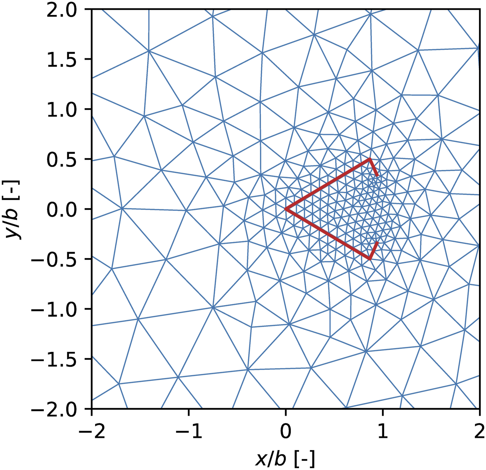
The wave input are from Chang et al. (2012), with a non-dimensional wavenumber kh = 0.65 [-], corresponding to L = 129.5 [m]. The linear wave height is set to H = 1.295 [m], and the simulations are run for 10 periods. For each incident angle, θ = {0°, 30°, 60°}, we compute the variation in η at each grid point (x
i
, y
i
) as
The corresponding non-dimensional quantity η
v
/H is visualized as contour plots in Appendix B (Figures 16–18). In Figure 14, we present η
v
/H along the UBA and LBA for the three wave angles, comparing our numerical results (LPF-θ) with digitized reference data from Chang et al. (2012) (C12-θ). Despite small differences arising from the use of finite-thickness structures, domain discretization, and minor wave reflections at the boundaries, the numerical solutions show good qualitative agreement with the reference results. This highlights that the incident angle affects the wave elevation in the vicinity of the breakwater structure, e.g., which may be of interest for sea-state or load estimations on the structure. Added to the figure, we also show the results from the FNPF model (FNPF-θ) with the same wave input parameters; however, with an incident wave of ɛ/ɛmax = 18%. From the figure, the added nonlinearity is visually evident in the maximum variance of the free surface elevation on the structure, especially on the LBA side. For θ = 60° on the UBA side, only a minor change can be observed; however, that is also the side completely sheltered from the incident waves. Breakwater solution (non-dimensional free surface variation) on the UBA and LBA for θ = {0°, 30°, 60°} using proposed linear (LPF-θ) and nonlinear (FNPF-θ) numerical model and results from Chang et al. (2012) (C12-θ).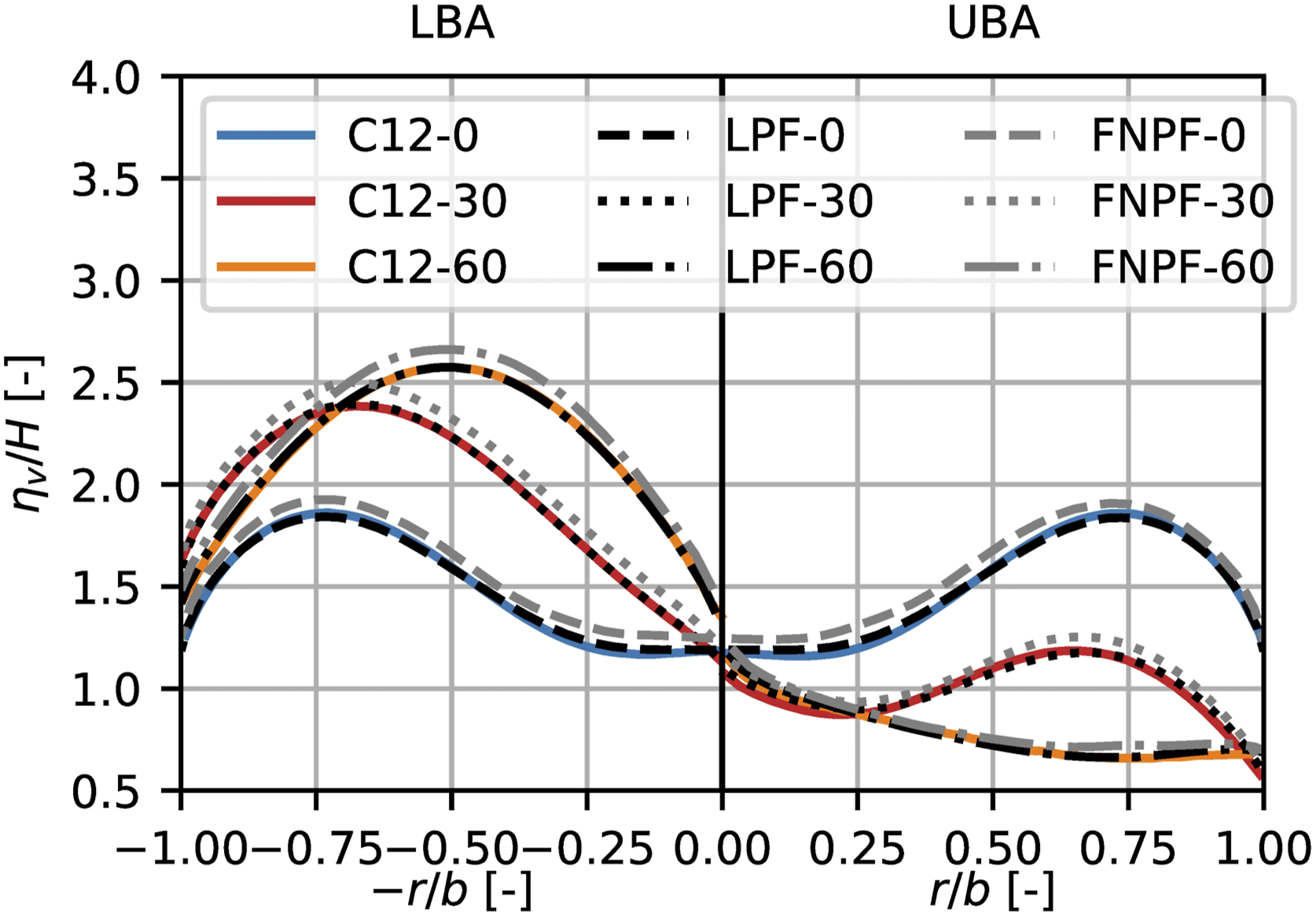
5. Conclusion
In this paper, we presented a new parallel implementation of a linear and fully nonlinear potential flow model, FNPF-SEM, to simulate wave propagation and wave-structure interaction. The model employs high-order (spectral) finite elements within the open-source Firedrake framework, leveraging its native MPI-based parallelism to handle large-scale computations efficiently. We detailed the mathematical formulation, including the governing equations, domain definitions, and numerical discretization. Parallel performance was assessed through code profiling for strong- and weak-scaling studies, demonstrating good parallel efficiency, particularly for large-scale simulations. Profiling confirmed that the Laplace problem constitutes the dominant computational cost. The numerical accuracy of the implementation was verified through convergence studies, confirming the expected algebraic and spectral convergence under mesh refinement and increased polynomial order, respectively. Finally, the model was compared against analytical solutions and experimental data for a range of wave-propagation and wave-structure-interaction scenarios, including high-order harmonic generation over a submerged bar and linear and nonlinear wave interactions with a vertical cylinder and a V-shaped breakwater. These results confirm the accuracy and applicability of the proposed framework. In ongoing work, the tool will be expanded to handle regional-scale wave propagation for accurate sea-state estimation and to consider areas with irregular coastlines, exploiting the advantages of unstructured meshes.
Footnotes
Acknowledgements
The research was carried out at the Technical University of Denmark (DTU) in the Department of Applied Mathematics and Computer Science, with computational resources provided by the DTU Computing Center (DCC). Lastly, the authors express their gratitude to the Firedrake team led by Professor David Ham for their support.
Funding
The authors disclosed receipt of the following financial support for the research, authorship, and/or publication of this article: This work partly contributes to the activities of the research project: “A new digital twin concept for floating offshore structures” supported by COWIfonden (Grant no. A-165.19) and partly the PhD-project of JV: “New Advanced Simulation Techniques for Wave Energy Converts”.
Declaration of conflicting interests
The authors declared no potential conflicts of interest with respect to the research, authorship, and/or publication of this article.
Data Availability Statement
The computational model developed in this study is publicly available on GitHub. The repository contains the full implementation, including source code, documentation, and example scripts necessary to reproduce the results presented in this paper. Additional information or clarification can be obtained from the corresponding author upon reasonable request. Link to GitHub: ![]()