Real time simulations of nuclear cloud rise with the energy research and forecasting model

Abstract

Operational models of nuclear cloud rise are required to have short simulation times to facilitate timely response by decision makers and emergency personnel. Because of this, current models are low dimensional approximations and rely on parameterized variables tuned to historical U.S. nuclear test results. These simplifications limit the capacity of current models to account for complex interactions with the local environment. As an alternative, this study examines the use of a new multiscale atmospheric solver, the Energy Research and Forecasting model (ERF), for use in fallout modeling applications. By simulating the fully three dimensional and time varying atmosphere dynamics, including turbulence with large eddy simulation (LES), significantly fewer modeling assumptions are required. In this study, four historical U.S. nuclear tests with varying heights of burst were simulated in ERF using an idealized setup and the results agree favorably with both historical test data and previous simulation data from the Weather Research and Forecasting model (WRF). Furthermore, it was demonstrated that cloud rise simulations could be performed faster than real time by leveraging GPU accelerated high performance computing resources with a combination of adaptive time stepping and adaptive mesh refinement. This represents a significant improvement in capability for nuclear cloud rise simulations and may enable the use of ERF as an operational tool in emergency situations.

Keywords

nuclear cloud rise large eddy simulation adaptive mesh refinement atmospheric models GPU WRF ERF

1. Introduction

In the event of a detonation or other release of radiological material, timely and accurate prediction of nuclear fallout patterns is a crucial component of disaster response. The National Atmospheric Release Advisory Center (NARAC) at Lawrence Livermore National Laboratory (LLNL) maintains a sophisticated suite of software that can be leveraged in the event of a disaster, such as the Fukushima Power Plant emergency in March of 2011 (Sugiyama et al., 2012). Rapid response to such disasters requires a predictive computational model with a short simulation time, to give as much time as possible for decision makers and emergency personnel to act. Current state-of-the-art operational models trade simulation fidelity for efficiency by utilizing low dimensional models with parameterized coefficients and can simulate nuclear cloud rise in minutes of computational time (Harvey et al., 1992; Norment, 1979). However, by definition, such models are unable to account for many complex environmental interactions, such as terrain, detailed weather or urban environments. These interactions affect nuclear cloud rise and the ultimate trajectory of the fallout patterns.

Previous work at LLNL (Arthur et al., 2021; Lundquist et al., 2023) investigated the use of the Weather Research and Forecasting (WRF) model’s Large Eddy Simulation (LES) (Skamarock et al., 2019) for nuclear cloud rise by simulating several historical U.S. nuclear tests. These studies demonstrated good agreement between the simulation data and published historical data, including late time cloud evolution and stabilized cloud height. Additionally, the WRF-Chem model (Grell et al., 2005) was adapted to simulate soil and bomb debris particle entrainment, which allowed for downstream fallout analysis with the Lagrangian Operational Dispersion Integrator (LODI) model (Nasstrom et al., 2007). While these studies proved that high resolution simulations of nuclear cloud rise and subsequent fallout are feasible with current technologies, the WRF model calculations required hours of wall clock time to simulate minutes of cloud rise. Ultimately, using the WRF model as a predictive tool for nuclear cloud rise in emergency response situations is not feasible without significant enhancements to its computational efficiency.

To address this gap in modeling, this study explores the Energy Research and Forecasting model (ERF;Almgren et al., 2023) for nuclear cloud rise applications. ERF is a new atmospheric LES code, drawing heavily from WRF’s numerical methodologies, but focusing on performance portability on exascale high performance computing (HPC) resources and greater flexibility in simulation capabilities. The model is built on top of AMReX (Zhang et al., 2019, 2021), a software framework for block-structured adaptive mesh refinement (AMR) applications. Preliminary results from the ERF model have demonstrated significant speedup in simulations utilizing graphical processing unit (GPU) resources compared to central processing unit (CPU) resources (Lattanzi et al., 2025).

A growing number of atmospheric codes have moved towards computing on GPU architectures, such as FastEddy (Sauer and Muñoz-Esparza, 2020), ClimateMachine (Sridhar et al., 2022), and PALM (Maronga et al., 2020), due to the capacity for computational speedup that has been observed in the field. For example, recent analyses have demonstrated potential speedups between 2.4 and 6x when using GPUs compared to CPUs, for the ClimateMachine model and FastEddy model, respectively. Accordingly, recent trends in HPC resources show that GPUs account for more than 90% of the available FLOPS (floating point operations per second) on the newest hardware, further reinforcing this trend away from traditional CPU-based computational methods.

The ERF model was chosen for the current study for several reasons. First, ERF is built on AMReX, a C++ software framework for writing massively parallel, performance portable applications for solving partial differential equations with AMR. This means that ERF is able to use CPU or GPU computation natively, without writing specialized GPU kernels. Furthermore, AMReX provides support for adaptive mesh refinement and Lagrangian particle tracking. Both features are of particular interest for cloud rise and fallout modeling applications. Cloud rise simulations stand to benefit from the use of AMR, because the feature of interest (i.e., the cloud) is typically small compared to the total size of the computational domain. In addition, Lagrangian particles can be used to simulate in-situ debris and soil particle entrainment and dispersion during cloud rise. This can allow for more accurate transport of radiological material in the cloud and stem resulting in higher fidelity input to the downstream modeling of radioactive particles. Finally, the use of a modular C++ interface makes ERF a highly customizable base for application-specific code development.

In this study, novel results from idealized nuclear cloud rise simulations with the ERF model are presented. Notably, the cloud rise was simulated faster than real time, i.e., the wall-clock time required for the simulation was less than the amount of time simulated by the model. This is a significant milestone for the use of high-fidelity models in emergency response scenarios and demonstrates the potential for more accurate methodologies to be adopted in the near future. The current study is organized as follows: In Section 2, the nuclear tests replicated in the ERF model are described along with the numerical methods and initialization procedure. In Section 3, cloud rise results from ERF are compared to previous results obtained from WRF (Arthur et al., 2021; Lundquist et al., 2023) and the differences between results from the two models are addressed. In Section 4, the computational performance on GPU architectures and the optimization strategies to simulate cloud rise faster than real time are discussed. Finally, the paper concludes in Section 5 with a discussion of future work to incorporate additional physical effects within the ERF cloud rise framework.

2. Problem setup

2.1. Description of test cases

In this study, four U.S. atmospheric nuclear tests are simulated using the ERF model: Upshot Knothole – Dixie, Upshot Knothole – Encore, Upshot Knothole – Grable, and Teapot – Wasp. Individual details of each test are reported in Hawthorne (1979) and summarized in Table 1. These tests were selected for the current study due to the availability of WRF simulation data from previous studies of nuclear cloud rise. In particular, Arthur et al. (2021) simulated the Dixie, Encore, and Wasp tests, and Lundquist et al. (2023) simulated the Grable test. Using these same tests for the ERF simulations allows for a direct comparison of the computational results and offers an additional source of validation for the ERF model.

Table 1.

Conditions for each test simulated in this study, as provided by the U.S. Department of Energy (DOE) National Nuclear Security Administration (NNSA) (NNSA, 2015).

Case	Dixie	Encore	Wasp	Grable
Location	37.085, −116.020	36.798, −115.930	37.087, −116.023	36.798, −115.930
Date [d-m-y]	06-04-1953	08-05-1953	18-02-1955	25-05-1953
HOB (m AGL)	1835.5	738.5	232.3	159.7
Yield (kT)	11	27	1	15
SHOB [ m/kT^1/3]	825.3	246.2	232.3	64.8
Regime	1	2	3	4

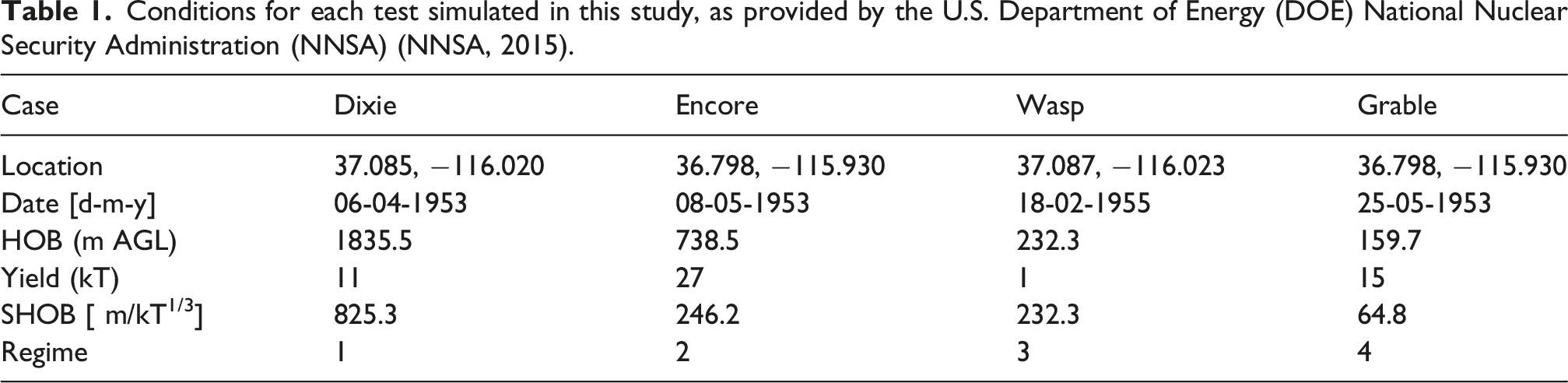
These four tests were selected for simulation with the WRF model for two primary reasons. First, available observational data from each test contains the complete time series data of the cloud top and bottom from detonation to the stabilization height (Hawthorne, 1979). Comparing simulation data to historical data provides an important method to validate the results of the ERF simulations over the full duration of cloud rise, as opposed to comparing against a single stabilized cloud height. Second, the four tests were chosen to represent a wide range of cloud behavior, which is typically characterized by a combination of the height of burst (HOB) above ground level (AGL) and device yield (Y) known as the scaled height of burst (SHOB), where

S H O B = H O B / Y^{1 / 3}

(Glasstone, 1977). According to Spriggs et al. (2020), cloud formation can be broken into eight separate regimes based on the behavior of the cloud, stem, and entrained dirt, which corresponds roughly to the SHOB (see Figure 1, Arthur et al. (2021)). For example, the Dixie test is a regime 1 burst (SHOB $> 457$ ), which is characterized by high altitude with no ground interaction and a slight stem formed by the device debris. In contrast, the Grable test is a regime 4 detonation (152 > SHOB > 61), which contains ground interaction including a reflected shockwave that distorts the initial fireball, soil particle entrainment, and slight cratering of the surface. The Encore and Wasp tests are categorized as regime 2 and 3, respectively, and the dynamics of the blast fall somewhere in between Dixie and Grable in terms of ground interaction and soil lofting. The four cases chosen for the present study represent a range of cloud behavior, useful for assessing current model capabilities and limitations.

Figure 1.

Horizontally averaged concentrations of the passive scalar field, C, as a function of vertical height from mean sea level (MSL) and horizontal distance in km. ERF model results are displayed in the left column, with WRF model results on the right. From top to bottom the tests are Dixie, Encore, Wasp, and Grable.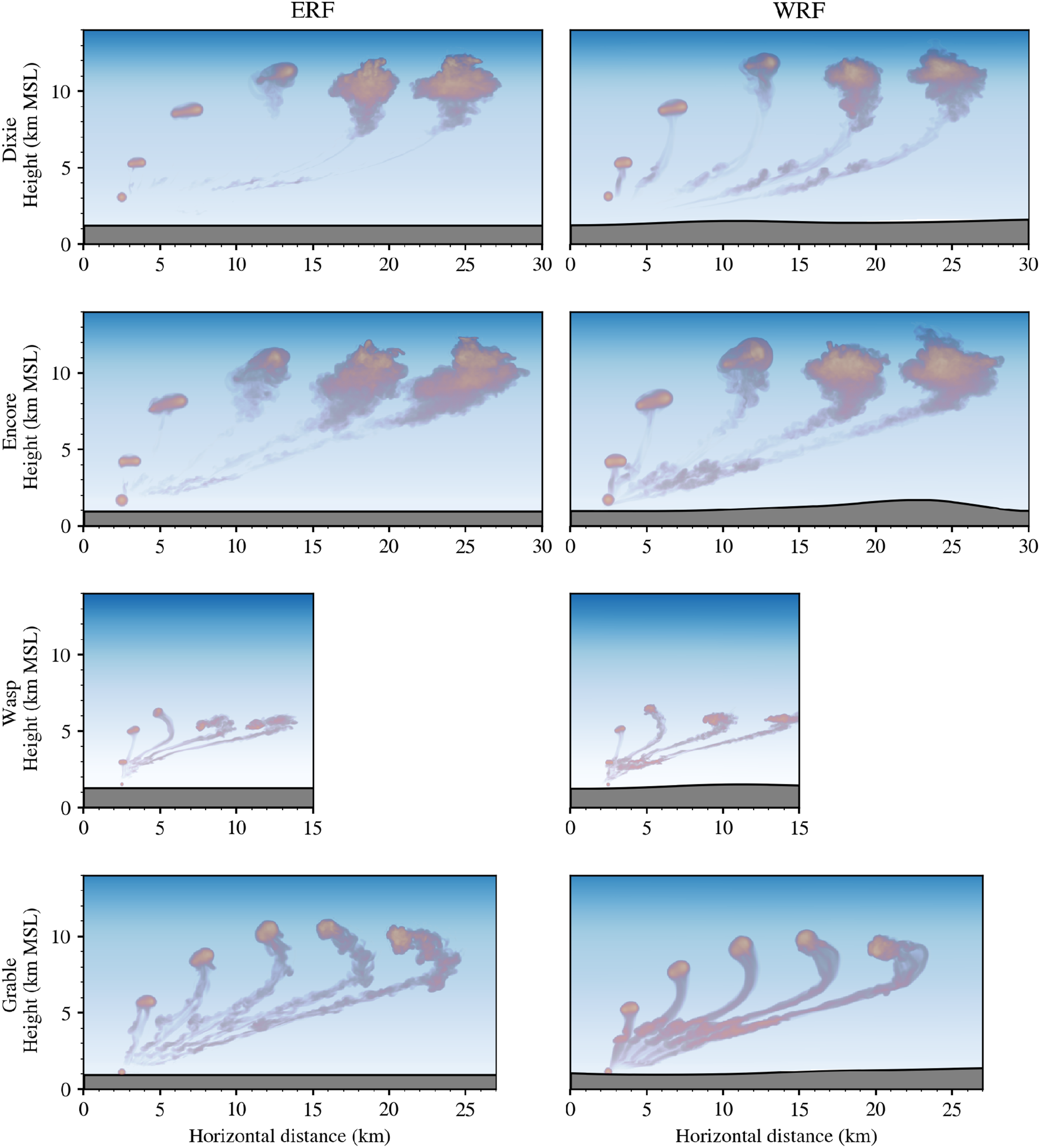

2.2. Numerical methods

ERF is an open source, multiscale atmospheric dynamics code that was originally sponsored as part of the U.S. Department of Energy’s Wind Energy Technologies Office. The code is developed on top of the AMReX software platform with high performance computing and performance portability in mind, allowing for a wide range of hardware configurations including GPU accelerators. Like WRF, ERF solves the fully compressible, three-dimensional Navier-Stokes equations for the moist atmosphere, with an Arakawa C-grid cell decomposition for spatial coordinates (Skamarock et al., 2019). Notably, ERF utilizes a height-based vertical coordinate rather than the pressure (or mass) based coordinate used by WRF.

The numerical discretization schemes available in ERF are designed to reflect available discretizations in WRF. For the results presented in Section 3, the spatial discretization is set to a fifth order upwind scheme in the horizontal direction and third order upwind in the vertical direction. A third order Runge-Kutta scheme with acoustic substepping is used for temporal discretization. The Deardorff turbulence model (Deardorff, 1980; Moeng, 1984) is used to compute the sub-grid stress in the LES closure, with a coefficient C_k = 0.1 to match the WRF simulations. In this configuration, the turbulent Prandtl number, Pr_t, is computed dynamically based on the grid spacing and mixing length.

Several simplifications have been made to the simulation setup to accelerate this initial validation of the ERF model for cloud rise simulations. First, instead of prescribing inflow/outflow conditions for the domain, periodic boundary conditions in the horizontal directions are used. The horizontal dimensions of the domain are sized such that the cloud will reach its stabilization height prior to reaching the domain boundaries, thus avoiding recirculation. Periodic boundary conditions must also be applied to the terrain; this is handled by setting a constant terrain height equal to the elevation at ground zero. This has only a minor effect on simulation results due to relatively small elevation changes at the test locations. Second, the air is assumed to be dry, and moisture models have been disabled. Arthur et al. (2021) examined the effects of latent heating and found that moisture had a negligible effect on cloud rise dynamics for the relatively dry atmosphere present in the Dixie, Encore, and Wasp tests. Third, a simple slip wall condition is used for the bottom boundary, with no land surface or boundary layer model. Despite the slip condition on the bottom wall, the initialization procedure (described below) factors in the surface friction which helps to ameliorate the effect of this simplification.

Despite the idealized nature of the present simulations, the direct simulation of cloud rise physics is significantly more complex than the operational models currently in use. The primary goal of the present study is to validate the capability of the ERF model to simulate nuclear cloud rise on timescales relevant to emergency response scenarios. Ultimately, future simulations of cloud rise in ERF will include more physical boundary conditions and microphysical models.

2.3. Initial conditions

For the cloud rise simulations in the current study, the base state of the atmosphere is initialized using an input sounding. With this option, a 1D input sounding file is supplied to ERF which specifies the potential temperature, θ and horizontal velocities U and V, as a function of height, as well as surface level values of θ and pressure, P. Based on these quantities, the hydrostatic base state of the atmosphere can be constructed, which is assumed to be uniform in the horizontal (x, y) directions.

The input sounding profiles utilized in the present study are taken directly from WRF simulations of Arthur et al. (2021) and Lundquist et al. (2023). In those studies, data from the National Centers for Environmental Prediction (NCEP)/National Center for Atmospheric Research (NCAR) Reanalysis Project (Kalnay et al., 2018) was used to perform a full weather simulation over the western half of the United States, which was then downscaled to the LES grid where the cloud rise simulations were performed. These vertical sounding profiles from ground zero were found to match closely with the measured soundings at the test sites, lending confidence to the accuracy of the reanalysis data.

Once the background atmospheric state has been calculated from the input sounding, a thermal bubble representing the detonation can be defined and superimposed on the background atmospheric state centered at the HOB, following previous studies (Arthur et al., 2021; Lundquist et al., 2023). A trigonometric profile is assumed for the temperature field inside the bubble, such that it decreases smoothly from the peak temperature to the ambient background state. The profile is defined as

θ^{'} (r) = \frac{θ_{0}}{2} (\cos (π r / R) + 1),

where θ′(r) is the temperature perturbation as a function of position, r, θ₀ is the peak perturbation temperature, and R is the radius of the bubble. For the present simulation, the peak temperature of the thermal perturbation is selected to be θ₀ = 1000K, which coincides with the peak temperature of previous WRF simulations.

To compare with historical test data, the thermal energy inside the initial bubble is set to a fraction of the reported device yield. According to Glasstone (1977), approximately 1/3 of the device yield is converted to thermal energy in the surrounding air for high-altitude bursts, which is the value used for the Dixie, Encore, and Wasp tests. Low altitude bursts, however, will preferentially heat the ground, causing less thermal energy to be absorbed by the surrounding atmosphere. Because of this, the initial bubble for the Grable test is assumed to contain only 1/6 of its yield as thermal energy.

With the thermal energy and peak temperature selected for each test, the bubble radius is determined through an iterative procedure. Given an initial guess for the bubble radius, the thermal energy inside the bubble is computed and compared to the desired energy based on the device yield, which is used to adjust the value of R until the computed and desired thermal energies are within a specified tolerance of 10⁻² kT. The initial bubble radius and peak temperature for each test simulation can be found in Table 2.

Table 2.

Simulation parameters for each of the test cases studied: Number of cells in horizontal (N_x, N_y) and vertical (N_z) directions, isotropic grid spacing Δx = Δy = Δz, simulation final time t_sim, bubble radius R, and peak bubble temperature θ₀.

Test	N_x × N_y × N_z	Δx (m)	Δt (s)	t_sim (s)	R (m)	θ₀ (K)
Dixie	756 × 360 × 396	40	0.05	720	375	1000
Encore	828 × 468 × 432	40	0.05	780	475	1000
Wasp	504 × 648 × 540	30	0.05	900	155	1000
Grable	432 × 684 × 360	40	0.05	600	310	1000

To preserve the equation of state, the density of the air inside the thermal bubble is decreased to account for the increased temperature, with the assumption that the pressure field has recovered to its initial atmospheric state at this stage of the detonation. In the previous WRF simulations, the reduction of air mass inside the vertical atmospheric columns due to the decreased density could cause significant distortion in the vertical grid spacing. Because of this, a secondary hydrostatic rebalance procedure was required to ensure that the vertical grid remained smooth in the region of the thermal bubble and a maximum peak temperature of θ₀ = 1000K was used. Because ERF uses a height-based vertical coordinate, this second hydrostatic rebalance is no longer necessary, as the grid does not deform in the presence of the fireball. Furthermore, preliminary studies suggest that cloud rise simulations may be stable up to θ₀ = 5000K, which may further improve comparison to historical data.

In addition to the temperature perturbation, a passive scalar field, C, is initialized to coincide with the initial temperature perturbation, i.e.,

C (r) = \frac{C_{0}}{2} (\cos (π r / R) + 1),

where the peak scalar concentration is C₀ = 100 kg/kg. The scalar does not affect the flow and is used as a tracer to both visualize and quantify cloud dynamics during the simulations. This is a valuable way of tracking the cloud evolution that does not rely on moisture microphysics models or other parameterizations to visualize and quantify the cloud rise dynamics. Future studies will incorporate the Lagrangian particle tracking in ERF to directly simulate soil and debris trajectories during cloud rise.

Simulation parameters for each of the four test cases are given in Table 2. The number of grid cells in the horizontal (N_x, N_y) and vertical (N_z) directions are given for each case. The total size of the computational domain is determined based on the vertical rise and downwind advection of the cloud. The grid spacing for each test is isotropic, i.e., Δx = Δy = Δz, with a nominal value of Δx = 40m for the Dixie, Encore, and Grable simulations. Due to the low yield of Wasp, the initial thermal bubble is much smaller than the other tests, so the grid spacing is decreased to Δx = 30m to ensure that the temperature field remains well resolved. Note that the Δx used in the present simulations for the Dixie, Encore and Wasp tests are larger than the grid spacing used in the WRF simulations (40m in ERF instead of 28.5 m in WRF for Dixie and Encore; 30m in ERF instead of 18.2 m in WRF for Wasp). Grid spacing was selected to balance both model accuracy and computational wall time. The time step of Δt = 0.05s is chosen to match the previous WRF simulations, which required small time steps at the beginning of the simulation to resolve the buoyancy-driven accelerations. While this is not necessary in the present simulations with ERF, the same time step is used in this section to facilitate comparison between the models; adaptive time stepping is explored in the next section. The duration of the simulations, t_sim, is set by how long it takes for the cloud to stabilize, which is determined using the available observational data for each test.

3. Comparison of ERF model to prior results

3.1. Qualitative comparisons

Qualitative comparisons between the idealized ERF model and previous results from WRF are shown in Figure 1. From top to bottom, the results from the Dixie, Encore, Wasp, and Grable tests are shown, with the idealized ERF results on the left and WRF results (Arthur et al., 2021; Lundquist et al., 2023) on the right. Due to the background flow, the cloud advects horizontally through the domain, which has been displayed from left to right in each panel for visual clarity. Images are produced by averaging the scalar field, C, in the horizontal dimension perpendicular to the direction shown, and then normalizing by the maximum value at each time step to aid in visualization. Additionally, several time steps have been included in each image to display the temporal evolution of the cloud. The background is colored by the potential temperature of the base state.

Overall, there is good agreement between the idealized ERF model results and previous simulations with WRF from a qualitative perspective. The cloud trajectories and heights are generally similar, reflecting the cloud’s interaction with the background velocity and pressure fields. Certain aspects, such as the tilt of the vortex core as it rises (e.g., in Dixie and Encore), or the advection of the stem past the cloud ‘top’ (e.g., in Grable), allow for identifiable features that are similar between the two models.

Some visual differences do exist between the two models, including the final cloud shape and the presence of a cloud stem, which deserve further discussion. First, given the idealized initial conditions used, it is not expected that the stabilized cloud shape in ERF will exactly match WRF. Due to the chaotic nature of turbulent flows, even similar initial conditions can result in markedly different features. In particular, it can be noted that the vortex core tends to break down into turbulence earlier in the ERF model than in the WRF model, despite both models using the same advection and time stepping schemes. This is most strongly observed in the Dixie and Encore cases, and could be due to differences in how the LES turbulence model is implemented or the underlying numerical dissipation, which controls the strength and size of small-scale flow features that govern the transition to turbulence.

The formation of a cloud stem is another difference between the ERF and WRF models. In the WRF model, cloud stems are clearly visible in all four tests, whereas the ERF model seems to lack a well defined stem for the Dixie and Encore tests; even the visible stems in the Wasp and Grable tests contain lower magnitudes of the scalar concentration relative to the cloud top. It is not immediately evident which model is more accurate in the cloud stem prediction because observational data are limited.

3.2. Quantitative comparisons

For a quantitative comparison between the ERF and WRF model simulations, a statistical estimate of the mean cloud height, h, is calculated for each test. The mean cloud height is computed by first obtaining a 1D representation of the vertical cloud distribution by averaging the scalar concentration, C (x, y, z), in the horizontal directions, i.e., 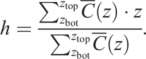$\bar{C} (z) = {⟨ C (x, y, z) ⟩}_{x y}$ to obtain a vertical profile. Then, a weighted average of the vertical direction is performed using the vertical cloud distribution as weights, such that

h = \frac{\sum_{z_{bot}}^{z_{top}} \bar{C} (z) \cdot z}{\sum_{z_{bot}}^{z_{top}} \bar{C} (z)} .

Here, z_bot and z_top correspond to the first and last grid cells in the vertical direction, respectively. Note that the bottom of the domain need not correspond to sea level. This calculation provides an estimate of the mean height at which the scalar is distributed within the cloud. The cloud stem is manually removed from the averaging process in an attempt to measure the height of the stabilized cloud only; this is of particular concern for the low altitude bursts of Wasp and Grable which have more prominent stems.

The results of this analysis are displayed in Figure 2, with the mean cloud heights plotted as a function of time for the Dixie, Encore, Wasp and Grable tests (from top to bottom). Note that the vertical coordinates differ between panels. Results from the present ERF simulations are shown in blue, with the WRF model results from Arthur et al. (2021) and Lundquist et al. (2023) in gray. Observed elevations of the cloud top and bottom from Hawthorne (1979) are given by the red lines. Due to the subjectivity inherent in the measurements of the cloud top/bottom, these should not be compared directly with the simulation results but instead are intended to give an upper and lower bound within which the mean cloud height is expected to be.

Figure 2.

Mean cloud height above ground level (AGL) as a function of time for the Dixie, Encore, Wasp, and Grable tests (top to bottom). ERF model results are given by the blue lines, prior WRF simulations are given by gray lines, and observational data of the cloud top and bottom from Hawthorne (1979) are given by red lines.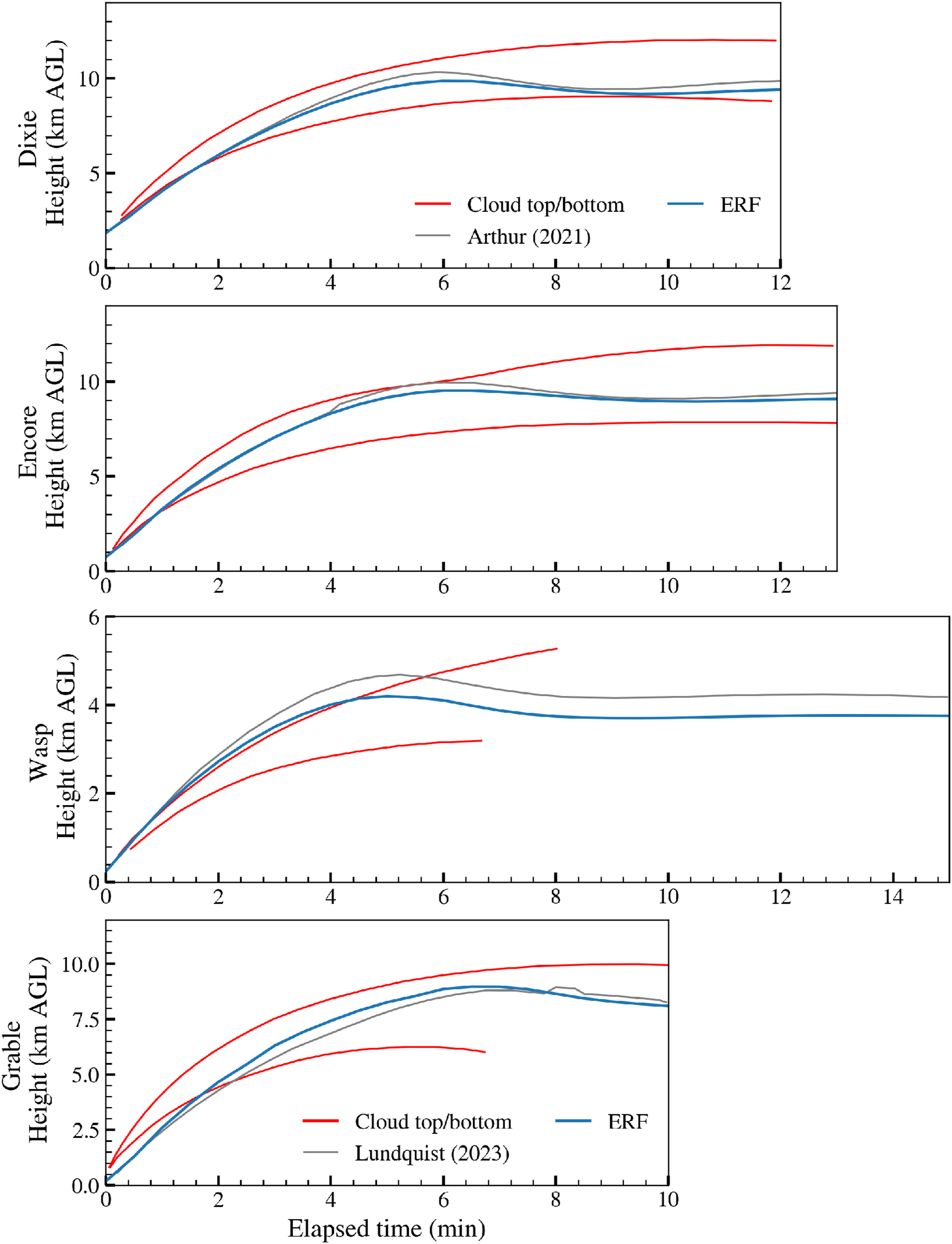

Overall, results of the mean cloud height demonstrate good agreement between the idealized ERF model and the WRF simulations. In the first three tests (Dixie, Encore, and Wasp), the WRF simulations exhibit a slightly faster rate of rise at early times and subsequently reach a higher peak altitude. Both models predict a subsequent decrease in the mean cloud height once reaching the peak, and the ERF model consistently produces slightly lower stabilized cloud heights. Mean cloud heights for both ERF and WRF are recorded in Table 3, as well as the percent difference between the predicted values of stabilized height between ERF and WRF, which range between 1.94 % (Grable) and 10.3% (Wasp).

Table 3.

Comparison of stabilized mean cloud heights between the WRF and ERF models, for each of the tests simulated in this study and the percent difference between them. Units for mean cloud height are in km above ground level (AGL).

Test	ERF	WRF	% diff.
Dixie	9.41	9.87	4.66 %
Encore	9.09	9.40	3.30 %
Wasp	3.75	4.18	10.3 %
Grable	8.10	8.26	1.94 %

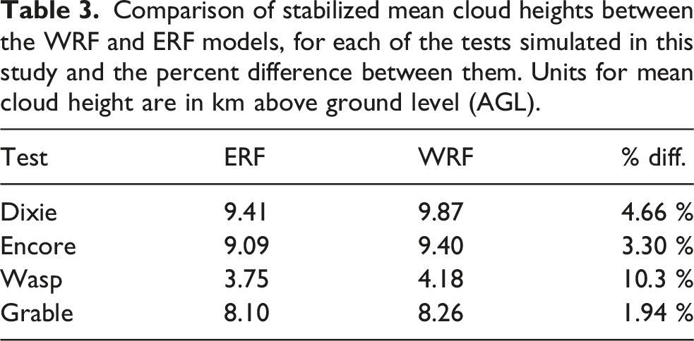
Notably, all of the predicted mean cloud heights fall generally within the observed boundaries of the cloud top and bottom. This is an important finding, because the cloud stabilization height is one of the most important features for predicting transport and dispersion of fallout after a nuclear detonation. Despite the simplifications in the setup, the mean cloud height predicted with ERF falls within the observed range for all tests.

Results from early times in the Grable test, i.e., t < 2 minutes, are notable because the predicted cloud height is below the observed cloud height. This is likely due to surface interactions; Grable has the lowest SHOB and the only bubble to intersect the bottom of the domain in the idealized initialization. Ground effects were examined in more detail by Lundquist et al. (2023), where the radiation-hydrodynamics code MIRANDA (Cook, 2007; Cook et al., 2021) was used to generate a more realistic initial condition of the Grable test (results not shown here). While this was found to improve the cloud rise prediction at early times, the stabilization height was unaffected.

4. Towards real time simulations

In the previous section, it was demonstrated that estimates of the mean cloud height with the ERF model are consistent with both the prior WRF simulation data and historical observations of cloud rise, providing confidence in the ERF model for cloud rise applications. In this section, the computational performance of the ERF model is discussed, with an emphasis on reducing simulation duration toward real time. A real time simulation is defined for this study as one in which the wall clock time of the simulation, t_wall, is equal to the amount of time simulated, t_sim. Faster than real time simulations are those where t_wall < t_sim. Three computational techniques are explored to accelerate the simulations: adaptive time stepping, strong scaling, and adaptive mesh refinement. Achieving real time (or faster) simulations would represent a significant milestone towards to the use of high-resolution atmospheric models for emergency response scenarios.

4.1. Adaptive timestepping

Simulation parameters are identical to the validation studies (refer to Table 2), with one exception; whereas a fixed time step was used in the above simulations to facilitate comparison to previous studies in WRF, the simulations in this section use adaptive time stepping to represent a more realistic use case and identify the fastest possible wall clock time for these simulations. For a compressible simulation such as the ones performed here, the time step Δt in ERF is computed dynamically each step using the Courant-Friedrich-Lewy (CFL) number,

Δ t = C F L \cdot m i n (\frac{Δ x}{| u | + c}, \frac{Δ y}{| v | + c}),

where |u| and |v| are the magnitude of the fluid velocity in the horizontal directions, c is the speed of sound, and Δx and Δy are the grid spacing in the horizontal directions. The vertical velocity is not included in this calculation because it is treated implicitly in the present formulation of the governing equations. The minimum value of Δt used for the timestep is computed across all grid cells in the domain.

By default the CFL number is set to 0.8, but it was found that, with the use of acoustic substepping, the present simulations were stable and accurate up to CFL = 2.6 for the Dixie, Encore, and Grable tests, and CFL = 2.5 for Wasp. The minimum number of acoustic substeps per time step is 4, corresponding to an acoustic CFL number of 0.65. This is consistent with the theoretical maximum CFL number of $1 / \sqrt{2}$ for the third order Runge-Kutta method used in ERF Skamarock et al. (2019). Note that all I/O operations, such as checkpointing and writing plot files are disabled for this study (except for the first and last time steps).

Enabling adaptive timestepping yields a significant increase in simulation performance. For the Dixie test, the value of Δt increases from a minimum of 0.15 seconds at the initial timestep to a final value of 0.297, resulting in a speedup of 5.6× compared to the baseline simulations presented in the prior section. However, the timestep used for the baseline simulations is a conservative value of Δt, so that this speedup may not be representative of a typical experience. For a more realistic estimate of the speedup, we compare the simulation times using the initial Δt = 0.15s compared to the adaptive timestepping procedure. This comparison yields a more modest, but noticeable, speedup of 2.0×.

4.2. Strong scaling performance

The most straightforward approach to reduce the wall clock time of a simulation is to increase the number of processors used in the simulation while keeping the total number of grid cells fixed. As such, a classical strong scaling study is performed for each of the four test cases (described above) to quantify the parallel scaling performance of the ERF code. Note that the adaptive timestepping, as described above, is used for this strong scaling study.

Strong scaling studies were performed on the Lassen supercomputer at Lawrence Livermore National Laboratory (LLNL). Each node on Lassen contains two IBM Power9 processors with 22 CPU cores (two cores are reserved for system processes) and 256 GB of DDR4 memory. Additionally, each node contains four NVIDIA Tesla V100 GPUs with 16 GB of high bandwidth memory. The GPUs are connected to the node with NVLINK 2.0 interconnect, and nodes are connected with a Mellanox 100 Gb/s Enhanced Data Rate InfiniBand network. Due to the configuration of Lassen, the GPUs provide the vast majority of the computational power (greater than 90% of the theoretical floating point operations). To provide a baseline comparison, strong scaling using CPUs was also tested using the Dane supercomputer at LLNL. Each node on Dane contains two 56-core Intel Sapphire Rapids processors with 256 GB of DDR5 memory, and a Cornellis Networks OmniPath high speed connection between nodes.

For the present study, the number of nodes used for each test is varied from 4 to 32, with a corresponding range of 16 to 128 GPUs on Lassen and 448 to 3584 CPU ranks on Dane. Performance is assessed by measuring the normalized wall time, t_wall/t_sim, where a value of 1 represents a real time simulation and values $< 1$ run faster than real time.

Normalized wall times as a function of the node count are presented in Figure 3, with the CPU scaling presented as a dotted line and the GPU scaling as solid lines. The horizontal dashed line at 1 represents the cutoff for a real-time solution. Finally, the gray dashed line represents the ideal strong scaling case. Of particular interest are the results from the Dixie and Grable GPU simulations, which are found to have normalized wall time values $< 1$ for simulations using more than 20 nodes (80 GPUs). However, it is found that the Encore and Wasp simulations, both of which contain a greater number of total grid cells compared to Dixie and Grable, fall short of the desired real time threshold even with 32 nodes (128 GPUs). Note that the Wasp test requires more wall time than Encore, despite having a similar number of grid cells. This is primarily because the Wasp test uses a smaller Δx, which reduces the timestep accordingly based on the CFL number.

Figure 3.

Normalized wall time (t_wall/t_sim) for each of the test cases described in Table 2, as a function of the number of nodes used for the simulation. The gray dashed line indicates ideal strong scaling. Values falling below the black dashed line at 1 indicate simulations faster than real time.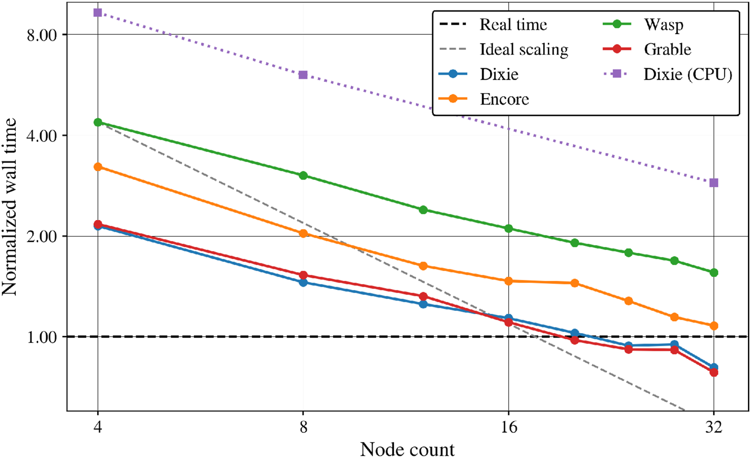

From these data, the strong scaling efficiencies are calculated using the 4 node simulation as a baseline. On the CPU, the strong scaling efficiency at 32 nodes was calculated to be 40%, which is comparable to the GPU strong scaling which ranges from 33 to 37% (depending on the test case). Compared to Figure 19 of Lattanzi et al. (2025), the CPU scaling efficiency is lower than expected based on the reported 60% scaling efficiency at 32 nodes. Interestingly, the GPU strong scaling in the present study is higher than the 20% efficiency reported in the same figure using 32 nodes. CPU/GPU speedup can also be calculated using these results, which was found to vary from 4.3x to 3.6x from 4 to 32 nodes. This speedup is smaller than the reported values from Figure 19 of Lattanzi et al. (2025) for 4 nodes (9.99x), but almost identical for 32 nodes (3.56x). The observed differences in scaling and speedup can be explained in part by differences in the computational setups (e.g., the results presented here utilize more cells per rank) and the LLNL and the National Energy Research Scientific Computing Center (NERSC) system hardware (e.g., NVIDIA V100 versus A100 GPUs).

The GPU scaling results presented here generally agree with prior studies of GPU enabled solvers in the literature (Häfner et al., 2021; Norman et al., 2022) and another AMReX-based compressible flow solver (Henry De Frahan et al., 2023). Due to increased computational performance, GPUs tend to expose more communication latency during parallel simulations compared to CPUs, which contributes to the relatively poor strong scaling efficiency compared to CPU codes. Additionally, as the workload on each GPU decreases, overhead associated with launching a kernel can become appreciable to the computational time, further limiting the parallel efficiency of the GPU simulation.

While sufficient strong scaling may allow for real time simulations of all the cases tested here, it is not guaranteed and will require significant computational resources. In an emergency response scenario, the cloud rise simulations would ideally use only a small number of resources and be included as an ensemble of many calculations run in parallel with varied initial parameters. For this use case, the adaptive mesh refinement capability can provide further computational gains on fewer compute resources.

4.3. Adaptive mesh refinement

The adaptive mesh refinement capability in ERF is provided via integration with the AMReX software framework. ERF employs a two-way coupling between coarse and fine patches in order to generate a consistent solution across AMR levels. Additionally, temporal subcycling enables advancing finer patches with smaller time steps than coarser patches. Significant work has gone towards ensuring conservation between coarse and fine patches such that the governing atmospheric flow equations are preserved throughout the simulation domain (Lattanzi et al., 2025). ERF supports up to 10 AMR levels with arbitrary integer refinement ratios between each level. Notably, ERF allows for refinement in both horizontal and vertical directions independently, allowing significantly more flexibility in grid generation compared to typical atmospheric flow solvers.

The cloud rise simulations described here are a particularly promising use case for AMR for two key reasons. First, the region of interest (i.e., the cloud) is small compared to the size of the computational domain at any given time step, which can significantly reduce the number of grid cells needed for the simulation. Second, the cloud is seeded with a scalar field at t = 0 which visually tracks the cloud throughout the simulation, providing an obvious and simple choice of location to refine the adaptive mesh. These are not generally true of atmospheric simulations, which may need additional calculations to identify regions that require increased mesh resolution. Moreover, the identified regions may account for a significant amount of the total computational domain size.

AMR simulations with adaptive time stepping were carried out for each of the historical nuclear tests described previously, using 2 levels of mesh refinement with a refinement factor of 3 between each level. The finest level of the AMR simulation is set to have the same grid spacing as the previous simulation, resulting in the level 0 (base) grid spacing increasing from 40 m to 360 m for the Dixie, Encore, and Grable simulations and from 30 m to 270 m for the Wasp simulation. The scalar field C is used as the refinement criteria with a threshold value of 0.01 to trigger the mesh refinement. The grid efficiency, ɛ, which controls how closely the AMR patches conform to the refinement criteria, is ɛ = 0.3. The number of timesteps between remeshing the AMR patches (regrid interval) is set to 6, and a buffer region of 4 grid cells is used between each each AMR level. The effect of ɛ and the buffer region on the simulation will be discussed in further detail in the following section.

The temporal evolution of the cloud and AMR patches for the Dixie test are shown in Figure 4. Individual AMR levels and patches can be observed to conform to the scalar isosurface throughout the duration of the simulation. Note the reduction in volume of the finest (level 2) grid compared to the total computational domain. At t = t_sim, the total number of grid cells (including levels 0 through 2) is 6.18 million compared to ≈ 108 million in the original simulation, a 95% reduction. The vast majority (87.9%) of these grid cells are concentrated in level 2 at the highest resolution. On a per-level basis, 15.0% of the level 0 grid cells are refined to level 1, and of those grid cells approximately 33.6% have been further refined to level 2, accounting for the reduction in total grid cells. Wall clock times for the AMR simulations are reported in Table 4.

Figure 4.

3D snapshots of the Dixie simulation at t = 0, 240, 480, and 720 seconds with AMR enabled and ɛ = 0.3. The cloud is visualized by an iso-surface corresponding to a value of C = 0.01, with the AMR patches overlaid onto the image. A 2D projection of the scalar field in the vertical direction is displayed at z = 0. The background is colored by the potential temperature.

Table 4.

AMR simulation results for each of the test cases studied: Wall clock time, t_wall, simulated time t_sim, normalized wall clock time t_wall/t_sim. All simulations used 8 nodes (32 GPUs) on Lassen and grid efficiency ɛ = 0.3.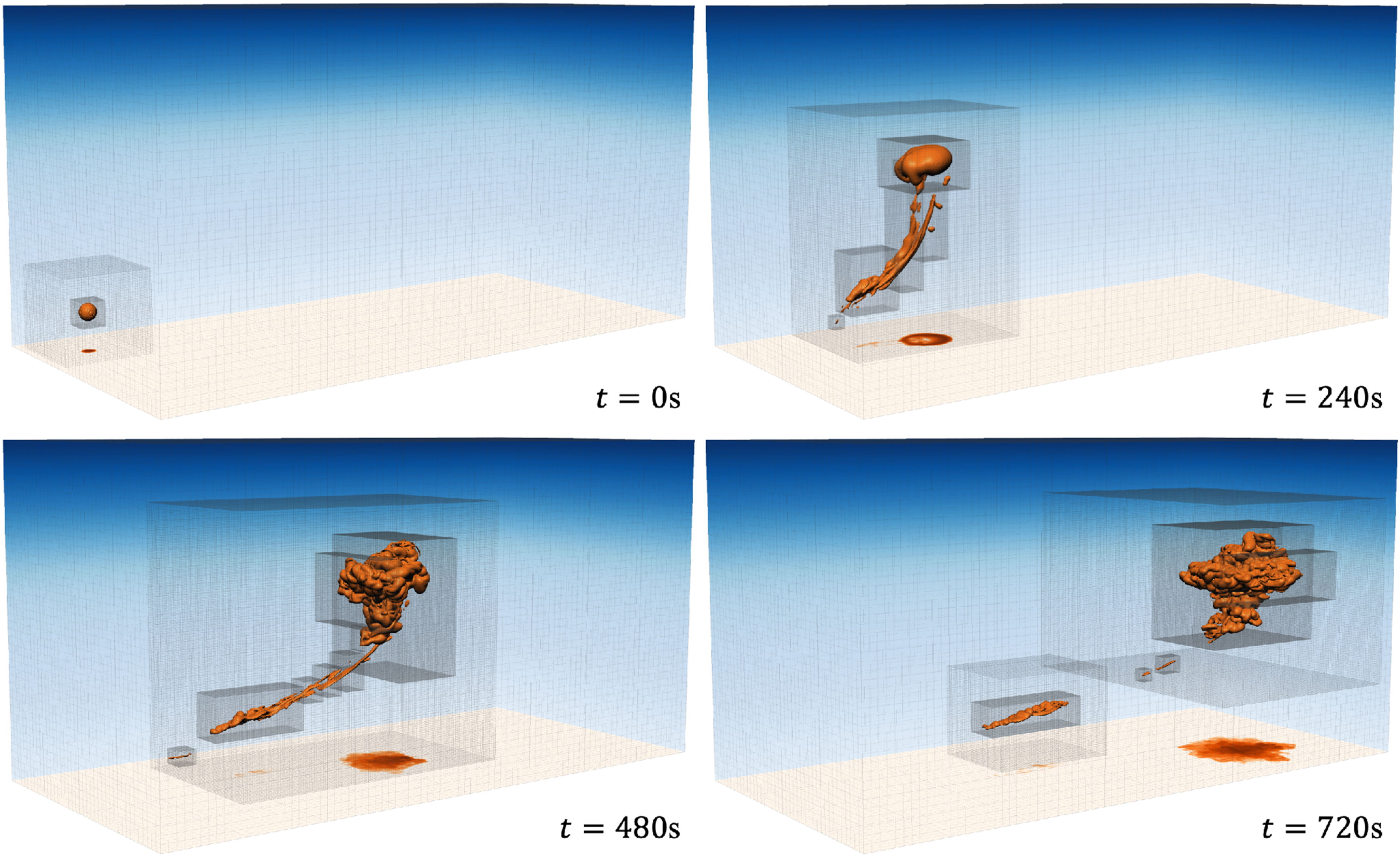

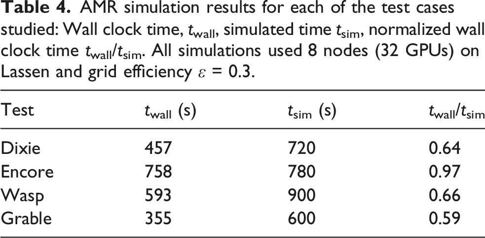
Test	t_wall (s)	t_sim (s)	t_wall/t_sim
Dixie	457	720	0.64
Encore	758	780	0.97
Wasp	593	900	0.66
Grable	355	600	0.59

Using only 8 nodes (32 GPUs) on Lassen, the reduction in total grid cells from AMR is sufficient to achieve normalized wall times $\leq 1$ for all four tests. Not only are the simulations faster than real time, they require one quarter (or less) of the compute resources compared to the non-AMR simulations.

The Dixie, Wasp, and Grable tests showed the greatest improvement from AMR, with normalized wall clock times between 1/2 and 2/3 of real time. Encore requires notably more time, despite reaching the real time threshold. This is likely due to the fact that, as the test with the largest yield, it requires more grid cells to capture the entire cloud. This could be accounted for by increasing the grid spacing at the finest level, or by using more GPUs to compensate for the higher workload.

In addition to simulating cloud rise in real time, it was found that using AMR had a negligible effect on simulation accuracy (depending on grid efficiency, see discussion below). Differences between the baseline ERF simulations and AMR ERF simulations range between 0.33 and 2.28%. The mean cloud height for the AMR simulations are compared to previous simulations in Figure 5.

Figure 5.

Mean cloud height as a function of time, as in Figure 2. Dashed lines correspond to cloud heights for AMR simulations with ɛ = 0.3.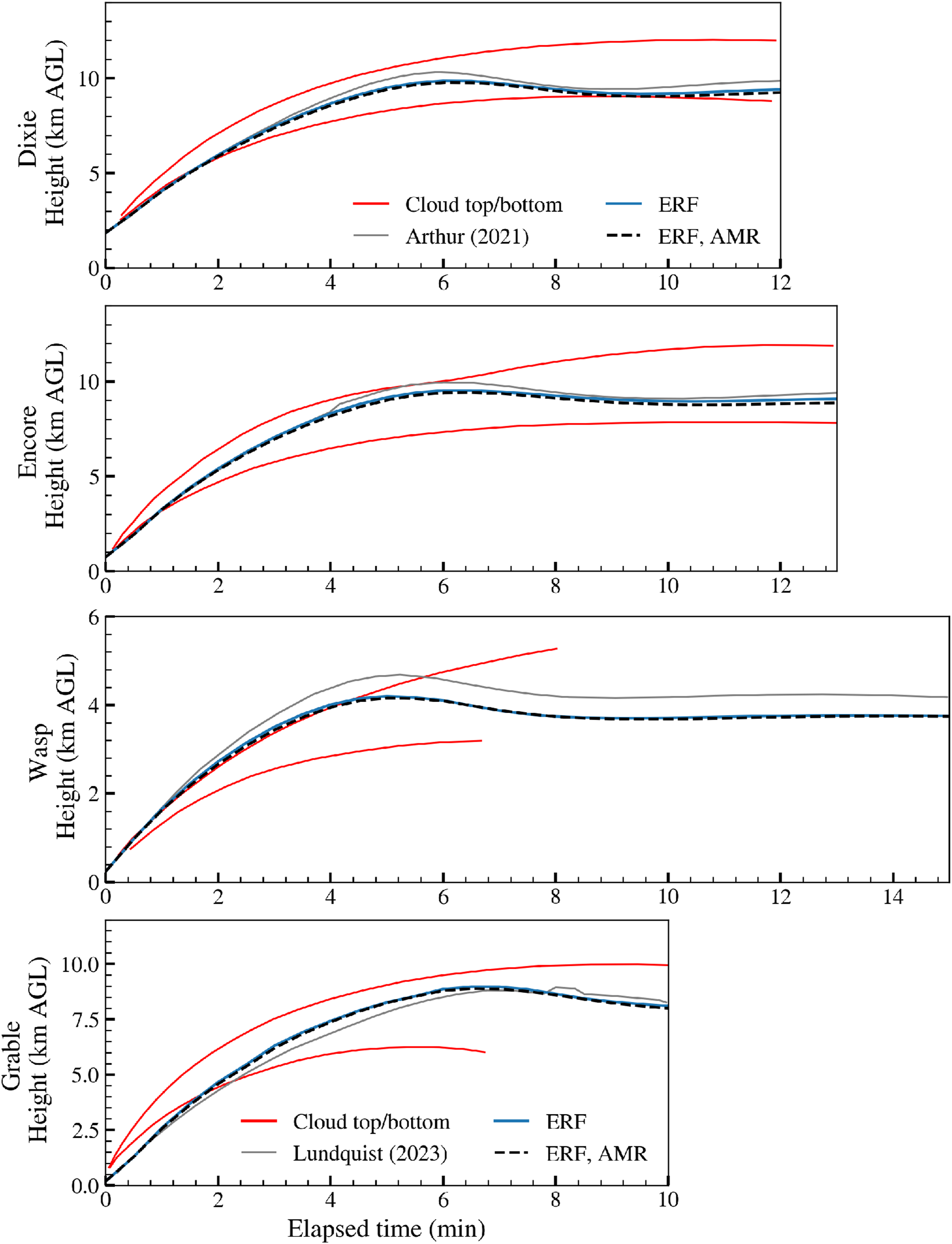

4.4. AMR grid efficiency

The AMR grid efficiency was found to have the largest single effect on both wall clock time and simulation accuracy. In the AMReX paradigm, the grid efficiency is a floating point value between 0 and 1 that determines how closely the AMR patches conform to the refinement criteria. For low grid efficiencies, fewer individual AMR patches are generated, increasing the amount of grid cells that fall outside of the refinement criteria. For grid efficiencies close to 1, many small AMR patches are generated such that they conform more closely to the refinement criteria threshold.

The effect of the grid efficiency on AMR patches can be observed in Figure 6, in which the mesh patches are visualized in the final time step of the Dixie test case for a range of grid efficiencies. The refinement criteria threshold is denoted by the orange isosurface of the scalar field, with a value of 0.01. It can be seen that, as the grid efficiency increases, the ratio of grid cells within the refinement criteria to the ratio of grid cells outside the criteria increases, which ultimately requires fewer overall grid cells. However, this comes at the cost of generating a larger number of smaller AMR patches.

Figure 6.

Snapshots of the mesh refinement structure at t_sim = 720s for the Dixie test case, using grid efficiencies 0.2, 0.4, 0.6, and 0.8.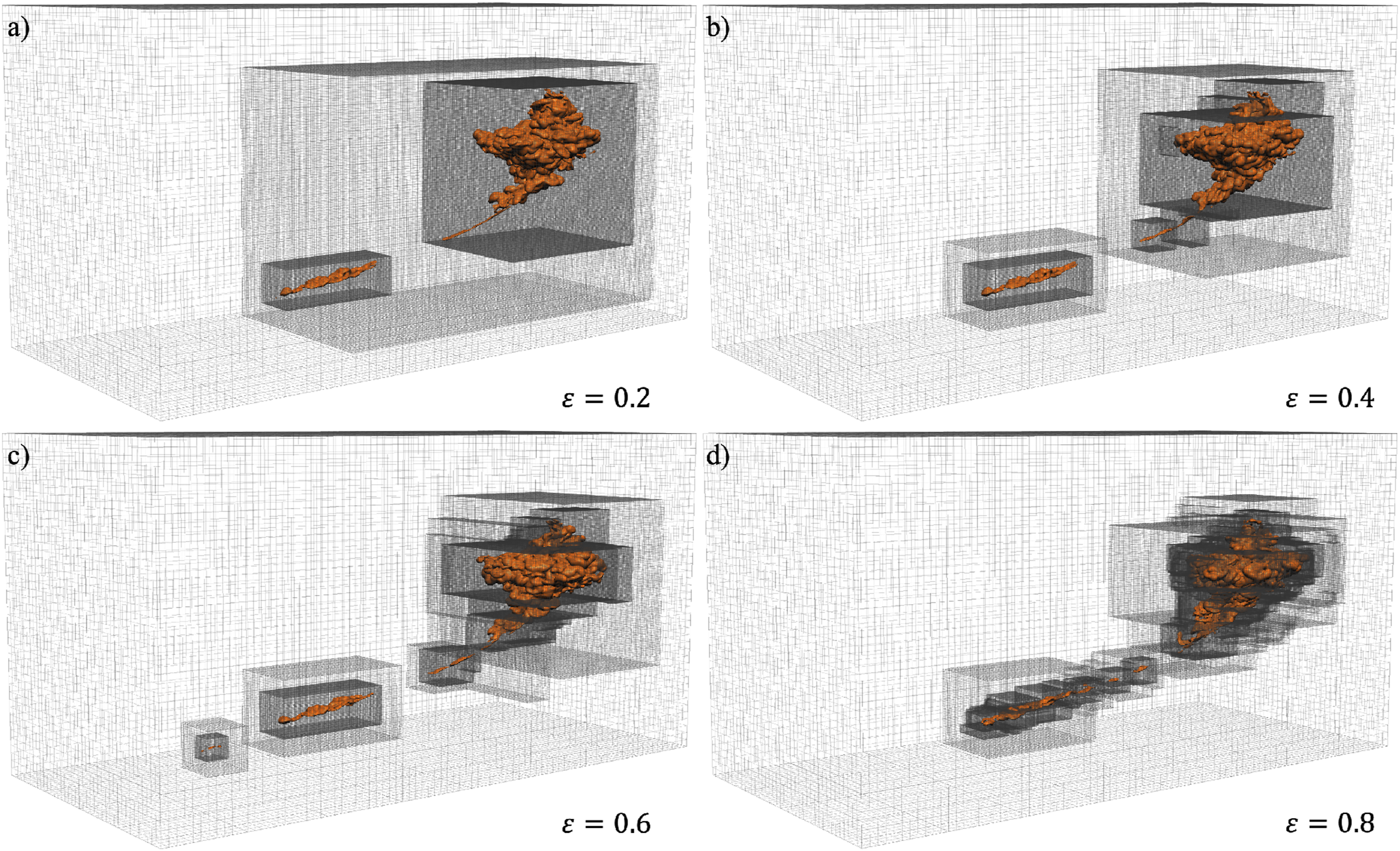

Despite the increased efficiency in grid cell count, it was found that larger values of grid efficiency could result in longer wall clock times, to the extent that the normalized wall time would actually increase with AMR enabled. In Figure 7, the normalized wall time on 8 nodes (32 GPUs) for each of the tests are plotted as a function of the grid efficiency. For all cases, ɛ < 0.5 results in wall times that are real time or faster. However, increasing the grid efficiency above 0.6 (or 0.5 for Encore) results in longer wall clock times and, in some cases, takes even longer than the non-AMR wall clock times. This is thought to be caused by the higher values of ɛ generating a greater quantity of smaller AMR patches, which could reduce GPU performance by limiting GPU concurrency and increased kernel launch overhead.

Figure 7.

Normalized wall clock time, t_wall/t_sim for each test as a function of the grid efficiency.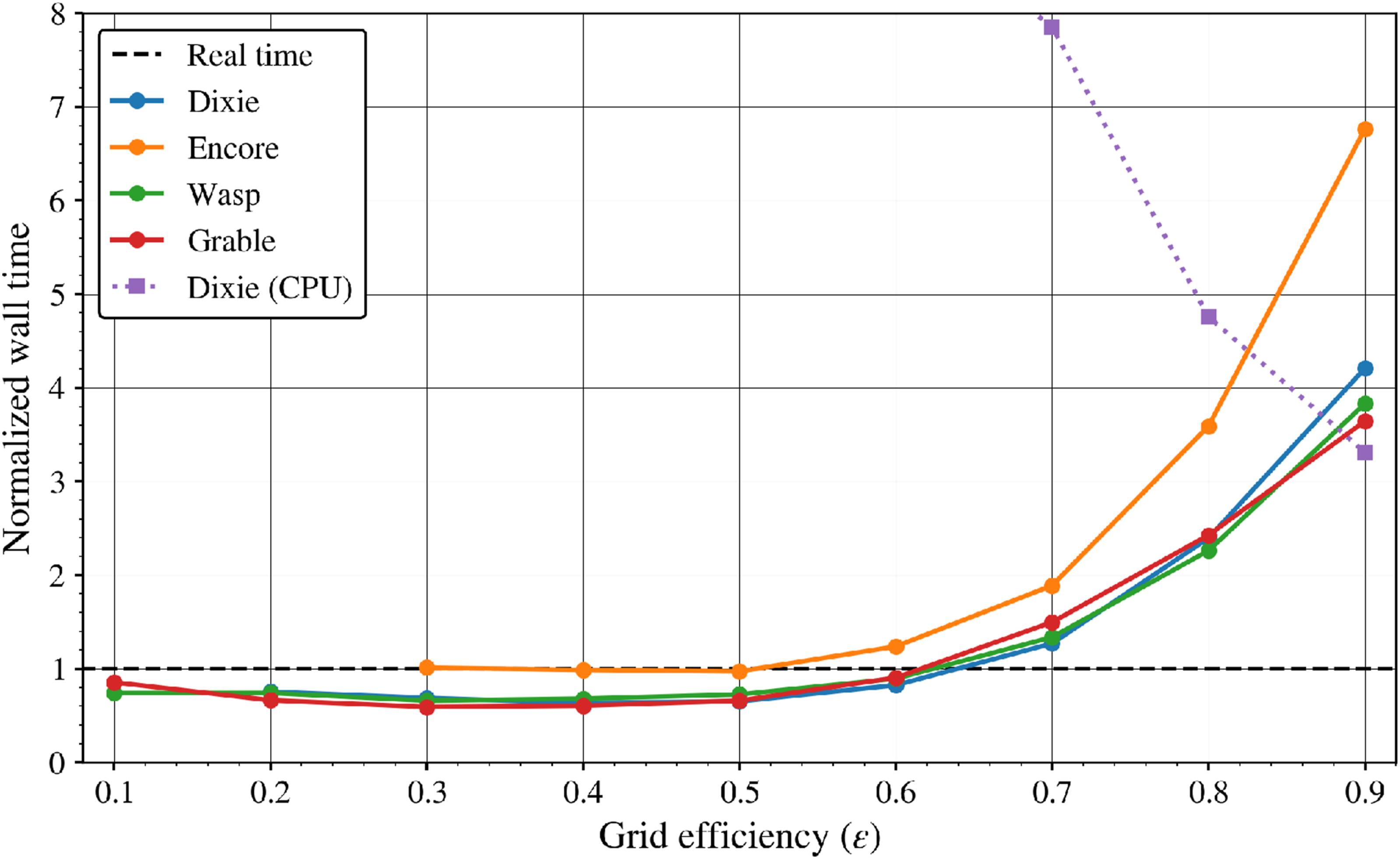

This is a notable result, as it goes against conventional AMR studies using CPU-based systems that typically demonstrate increased performance with increasing grid efficiency. To highlight this, a CPU simulation of the Dixie test using 8 nodes on the Dane supercomputer has been included in Figure 7 as a dotted line. Normalized wall times are comparable between CPU and GPU simulations for large values of the grid efficiency, with the CPU simulation even surpassing the GPU-enabled simulation time at ɛ = 0.9 with a normalized wall time of 3.3. However, the normalized wall times increase dramatically below ɛ = 0.8. This difference between CPU and GPU behavior highlights the unique challenges associated with optimizing simulation performance on a wide variety of systems.

Grid efficiency was also found to affect the solution accuracy, in combination with the regrid interval, i.e., the time interval between re-meshing the domain based on the refinement criteria. The regrid interval is a tunable parameter in the AMR settings, which should be small enough to ensure that the mesh is properly adhering to the refinement criteria, but large enough to prevent the re-meshing process from taking unnecessary computational time. A regrid interval of 6 steps was used for the simulations described here.

Especially for the cloud rise cases involving significant background advection, it was found that the larger grid efficiencies required short regrid intervals to prevent the cloud advecting out of the refined mesh at each time step. This has a compounding effect; not only do large grid efficiencies take longer to solve as shown in Figure 7, they also require more frequent re-meshing operations to preserve simulation accuracy. This could be remedied by adding a number of buffer grid cells outside of the refinement criteria, which is an independent parameter in the ERF input file. A buffer region of 4 grid cells is used in the present simulations; a larger number of buffer cells would increase the AMR patch size and allow more time between needing to re-mesh the solution (at the cost of additional grid cells). The size of the AMR patch is also affected by the blocking factor, an optional input parameter which requires that each AMR patch be a multiple of the given value. The blocking factor for the present simulations is 4. While these parameters were not analyzed in depth for the present work, this could be explored in the future to further improve AMR performance.

5. Conclusions and future work

This study represents a key breakthrough for high-fidelity nuclear cloud rise modeling enabled by the Energy Research and Forecasting model. Current operational capabilities are simplified to achieve real time computational speed, while higher-fidelity options are too computationally expensive for operational use. With the combination of GPU computing resources, adaptive time stepping, and adaptive mesh refinement, four historical U.S. nuclear tests were simulated faster than real time, i.e., the wall clock time necessary for a cloud rise simulation is less than the duration of the real cloud rise. This demonstrates a significant improvement over the current state-of-the-art modeling capabilities. Moreover, AMR-enabled cloud rise simulations in ERF were found to agree with both observational data from the nuclear tests as well as prior simulation data using the WRF model. These results have the potential to improve predictive capabilities in the event of a nuclear detonation by including fully 3D atmosphere dynamics, turbulence, and terrain effects into the cloud rise model.

Future work is focused on improving the accuracy and capability of the ERF cloud rise model in several ways. Current efforts are concentrated on including additional physics into the present cloud rise simulations, such as multiscale atmospheric dynamics, terrain interaction, and moisture effects. In addition, efforts are underway to improve simulation fidelity by coupling the initial condition in ERF to the output of a hydrodynamics solver that is capable of simulating the detonation and blast wave directly (Kanarska et al., 2009, 2020). In previous work, it was found that using a realistic initial condition (compared to the idealized bubble approach used here) can improve comparison to historical data (Lundquist et al., 2023). Finally, the native Lagrangian particle capability in AMReX is being expanded to use the super droplet method (Ghosh et al., 2025; McGuffin et al., 2022) for use in modeling fallout activity, transport, and dispersion. Ultimately, the inclusion of these features in ERF would allow for high-fidelity operational cloud rise simulations, which could lead to more accurate fallout predictions in emergency response scenarios.

Footnotes

ORCID iDs

Brandon C. Blakeley

Ann S. Almgren

David J. Gardner

Funding

The authors disclosed receipt of the following financial support for the research, authorship, and/or publication of this article: This work was performed under the auspices of the U.S. Department of Energy by Lawrence Livermore National Laboratory under Contract DE-AC52-07NA27344. BCB, RSA, DJG and KAL were supported by LDRD project 24-SI-001, “Accelerated Atmospheric Simulations for Rapid Response in Nuclear, Climate, and Energy-Security Applications”. The contributions of ASA and AML were performed under the auspices of the U.S. Department of Energy at the Lawrence Berkeley National Laboratory under contract DE-AC02-05CH11231. This article is approved for unlimited release as LLNL-JRNL-2012579.

Declaration of conflicting interests

The authors declared no potential conflicts of interest with respect to the research, authorship, and/or publication of this article.

Author biographies

Brandon C. Blakeley completed this work while a postdoctoral research fellow at Lawrence Livermore National Laboratory in the Computational Engineering Division. His research interests are in turbulent mixing and GPU computing, and his work has varied from aerospace applications to atmospheric models. Brandon received a PhD in Mechanical Engineering from the University of Washington.

Robert S. Arthur is a staff scientist in the Atmospheric, Earth, and Energy Division at Lawrence Livermore National Laboratory. His research focuses on high-resolution atmospheric modeling for energy and transport and dispersion applications. Through his affiliation with the National Atmospheric Release Advisory Center (NARAC), he supports research and development of nuclear effects models. Robert received his PhD in Civil & Environmental Engineering from Stanford University, and his BS in Engineering Science from the University of Virginia.

Aaron M. Lattanzi is a research scientist in the Applied Mathematics and Computational Research Division at Lawrence Berkeley National Laboratory. His research interests focus primarily on atmospheric and multiphase flows.Aaron received his MS and PhD in Chemical Engineering from the University of Colorado, Boulder and his BA in Chemical Engineering from the University of Washington.

Ann S. Almgren is a senior scientist in the Applied Mathematics and Computational Research Division at Lawrence Berkeley National Laboratory. Her research interests are primarily in computational algorithms and their high-performance implementation for solving PDEs in a variety of application areas, including ocean and atmosphere modeling. Ann received her MS and PhD in Mechanical Engineering from the University of California, Berkeley and her BA in Physics from Harvard University.

David J. Gardner is a computational scientist in the Center for Applied Scientific Computing (CASC) at Lawrence Livermore National Laboratory. His work focuses on the development, implementation, and deployment of accurate and efficient numerical methods for simulating multiscale, multiphysics applications on high-performance computing systems. He has collaborated with scientific teams across a range of application areas, including atmospheric dynamics, combustion, cosmology, additive manufacturing, quantum dynamics, and materials science. David received his Ph.D. in computational and applied mathematics from Southern Methodist University.

Katherine A. Lundquist leads the National Atmospheric Release Advisory Center (NARAC) at Lawrence Livermore National Laboratory. Katherine earned her Ph.D. and M.S. in mechanical engineering from the University of California, Berkeley and her B.S. in mechanical engineering at The University of Texas at Austin. She leads the development of NARAC’s models for atmospheric transport and dispersion and conducts research in scientific computing for atmospheric modeling applications.

References

Almgren

Lattanzi

Haque

, et al. (2023) ERF: energy research and forecasting. Journal of Open Source Software 8(87): 5202. https://doi.org/10.21105/joss.05202

Arthur

Lundquist

Mirocha

, et al. (2021) Simulating nuclear cloud rise within a realistic atmosphere using the weather research and forecasting model. Atmospheric Environment 254: 118363. https://doi.org/10.1016/j.atmosenv.2021.118363

Cook

(2007) Artificial fluid properties for large-eddy simulation of compressible turbulent mixing. Physics of Fluids 19(5): 055103. https://doi.org/10.1063/1.2728937

Cook

Bauer

Spriggs

(2021) The reflection of a blast wave by a very intense explosion. Proceedings of the Royal Society A 477(2250): 20210154. https://doi.org/10.1098/rspa.2021.0154

Deardorff

(1980) Stratocumulus-capped mixed layers derived from a three-dimensional model. Boundary-Layer Meteorology 18: 495–527. https://doi.org/10.1007/bf00119502

Ghosh

Beydoun

McGuffin

, et al. (2025) Super droplet method for lagrangian microphysics simulations in ERF. SIAM Conference on Computational Science and Engineering (CSE25), held in Fort Worth, TX from March 3–7, 2025.

Glasstone

(1977) The Effects of Nuclear Weapons. United States Department of Defense and the Energy Research and Development Administration.

Grell

Peckham

Schmitz

, et al. (2005) Fully coupled “online” chemistry within the WRF model. Atmospheric Environment 39(37): 6957–6975. https://doi.org/10.1016/j.atmosenv.2005.04.027

Häfner

Nuterman

Jochum

(2021) Fast, cheap, and turbulent—Global ocean modeling with GPU acceleration in python. Journal of Advances in Modeling Earth Systems 13(12): e2021MS002717. https://doi.org/10.1029/2021ms002717

10.

Harvey

Serduke

Edwards

, et al. (1992) KDFOC3: a nuclear fallout assessment capability. In: UCRL-52338. Lawrence Livermore National Laboratory.

11.

Hawthorne

(1979) Compilation of local fallout data from test detonations 1945-1962 – extracted from DASA 1251, volume I - continental US tests. Technical Report DNA-1251-1-EX, Defense Nuclear Agency.

12.

Henry de Frahan

Rood

Day

, et al. (2023) PeleC: an adaptive mesh refinement solver for compressible reacting flows. The International Journal of High Performance Computing Applications 37(2): 115–131. https://doi.org/10.1177/10943420221121151

13.

Kalnay

Kanamitsu

Kistler

, et al. (2018) The NCEP/NCAR 40-year reanalysis project In: Renewable Energy. Routledge. Vol1_146–Vol1_194.

14.

Kanarska

Lomov

Glenn

, et al. (2009) Numerical simulation of cloud rise phenomena associated with nuclear bursts. Annals of Nuclear Energy 36(10): 1475–1483. https://doi.org/10.1016/j.anucene.2009.08.009

15.

Kanarska

Dunn

Glascoe

, et al. (2020) Semi-implicit method to solve compressible multiphase fluid flows without acoustic time step restrictions. Computers & Fluids 210: 104651. https://doi.org/10.1016/j.compfluid.2020.104651

16.

Lattanzi

Almgren

Quon

, et al. (2025) ERF: energy research and forecasting model. Journal of Advances in Modeling Earth Systems 17: e2024MS004884, URL. https://doi.org/10.1029/2024MS004884

17.

Lundquist

Arthur

Neuscamman

, et al. (2023) Examining the effects of soil entrainment during nuclear cloud rise on fallout predictions using a multiscale atmospheric modeling framework. Journal of Environmental Radioactivity 270: 107299. https://doi.org/10.1016/j.jenvrad.2023.107299

18.

Maronga

Banzhaf

Burmeister

, et al. (2020) Overview of the PALM model system 6.0. Geoscientific Model Development 13(3): 1335–1372. https://doi.org/10.5194/gmd-13-1335-2020

19.

McGuffin

Lucas

Morris

, et al. (2022) Super-droplet method to simulate lagrangian microphysics of nuclear fallout in a homogeneous cloud. Journal of Geophysical Research: Atmospheres 127(18): e2022JD036599. https://doi.org/10.1029/2022JD036599

20.

Moeng

(1984) A large-eddy-simulation model for the study of planetary boundary-layer turbulence. Journal of the Atmospheric Sciences 41(13): 2052–2062. https://doi.org/10.1175/1520-0469(1984)041<2052:alesmf>2.0.co;2

21.

Nasstrom

Sugiyama

Baskett

, et al. (2007) The NARAC modeling and decision support system for radiological and nuclear emergency preparedness and response. International Journal of Emergency Management 4: 524–550.

22.

NNSA (2015) United States nuclear tests, July 1945 through September 1992, September 2015. Technical Report, US Department of Energy, Nevada Field Office. https://doi.org/10.2172/1351809. URL. https://www.osti.gov/biblio/1351809

23.

Norman

Bader

Eldred

, et al. (2022) Unprecedented cloud resolution in a GPU-Enabled full-physics atmospheric climate simulation on OLCF’s summit supercomputer. The International Journal of High Performance Computing Applications 36(1): 93–105. https://doi.org/10.1177/10943420211027539

24.

Norment

(1979) DELFIC: Department of Defense Fallout Prediction System. Volume I-Fundamentals, Bedford, MA. Atmospheric Science Associates.

25.

Sauer

Muñoz-Esparza

(2020) The FastEddy® resident-GPU accelerated large-eddy simulation framework: model formulation, dynamical-core validation and performance benchmarks. Journal of Advances in Modeling Earth Systems 12(11): e2020MS002100. https://doi.org/10.1029/2020ms002100

26.

Skamarock

Klemp

Dudhia

, et al. (2019) A description of the advanced research WRF version 4. NCAR Tech. Note NCAR/TN-556+STR 145.

27.

Spriggs

Neuscamman

Nasstrom

, et al. (2020) Fallout cloud regimes. Countering WMD Journal 21: 1771428, URL. https://www.osti.gov/biblio/1771428

28.

Sridhar

Tissaoui

Marras

, et al. (2022) Large-eddy simulations with ClimateMachine v0. 2.0: a new open-source code for atmospheric simulations on GPUs and CPUs. Geoscientific Model Development 15(15): 6259–6284. https://doi.org/10.5194/gmd-15-6259-2022

29.

Sugiyama

Nasstrom

Probanz

, et al. (2012) NARAC Modeling During the Response to the Fukushima Dai-Ichi Nuclear Power Plant Emergency. Livermore, CA. Lawrence Livermore National Laboratory (LLNL). URL. https://www.osti.gov/biblio/1035949

30.

Zhang

Almgren

Beckner

, et al. (2019) AMReX: a framework for block-structured adaptive mesh refinement. Journal of Open Source Software 4(37): 1370. https://doi.org/10.21105/joss.01370

31.

Zhang

Myers

Gott

, et al. (2021) AMReX: block-structured adaptive mesh refinement for multiphysics applications. The International Journal of High Performance Computing Applications 35(6): 508–526. https://doi.org/10.1177/10943420211022811