A GPU-accelerated simulation of rapid intensification of a tropical cyclone with observed heating

Abstract

This paper presents a limited-area atmospheric simulation of a tropical cyclone accelerated using GPUs. The OpenACC directive-based programming model is used to port the atmospheric model to the GPU. The GPU implementation of the main functions and kernels is discussed. The GPU-accelerated code produces high-fidelity simulations of a realistic tropical cyclone forced by observational latent heating. Performance tests show that the GPU-accelerated code yields energy-efficient simulations and scales well in both the strong and weak limit.

Keywords

tropical cyclone rapid intensification atmospheric model GPU acceleration

1. Introduction

Tropical cyclones (TCs) are a natural hazard that significantly impact human life and economies. Despite their huge impact, TC evolution is a physical process that is poorly understood. In particular, the prediction of TC intensity has been a challenging problem because of complexities in the multiscale interactions of convective-scale processes and synoptic-scale environment (Fischer et al., 2019). This is true especially when TCs undergo rapid intensification (RI), where TCs drastically intensify in a short period of time – typically change in wind speed of around 30 knots within 24 hours. To explore and study the RI mechanisms, we perform high-fidelity TC simulations. Modeling and numerical simulations of TCs can enhance our understanding of the underlying geophysical processes and may improve the accuracy of forecasts and risk assessment. However, one of the main challenges in the modeling of TC evolution is the high computational cost to resolve the fine-scale features needed for accurate prediction of TC intensity. To achieve computationally efficient simulations, we port a limited-area atmospheric model to the graphics processing unit (GPU) using a multi-CPU multi-GPU approach.

A nonhydrostatic atmospheric model is used to simulate TC evolutions. The code we use to perform these simulations is called xNUMA, a new version of the NUMA (Nonhydrostatic Unified Model of the Atmosphere) code (Giraldo et al., 2013; Kelly and Giraldo, 2012). The xNUMA code is designed specifically for a multiscale modeling framework (MMF) for atmospheric flows, and is written in modern Fortran using an object-oriented approach. Because all the spatial discretization and time-integration methods are encapsulated in the form of objects, it is capable of instantiating multiple simulations simultaneously during execution.

Previously, the NUMA nonhydrostatic atmospheric model, which employs element-based Galerkin methods, was ported to GPUs (Abdi et al., 2019a, 2019b) using OCCA (Medina et al., 2014). Various time integration methods, including explicit and semi-implicit schemes, were ported and demonstrated good scalability for numerical weather problems. However, using a hardware-agnostic application programming interface (API) like OCCA increases development complexity. It requires writing an entirely separate parallel branch of code in different languages, as well as modifying data structures and kernel execution patterns. In this work, we explore a hardware-specific directive-based approach to simplify offloading while maintaining performance.

In porting xNUMA to GPUs, we chose to approach the problem using a directive based implementation. The main advantage of directive-based approaches is the ability to easily make large GPU coding contributions to the code base while still maintaining a correct and performant CPU code base. In this work, we ported xNUMA to GPUs using the OpenACC programming standard (OpenACC Organization, 2020) as implemented in the NVIDIA compiler (NVIDIA Corporation, 2025).

High-order Galerkin methods are attractive for hurricane research due to their low numerical dissipation. An earlier study (Guimond et al., 2016) revealed that high-order methods better capture the vortex response to asymmetric thermal perturbations in hurricane RI due to reduced damping of heat and kinetic energies. Recently, an adaptive mesh refinement technique has been incorporated into the high-order Galerkin method to efficiently capture the fine features of hurricanes (Tissaoui et al., 2024).

High-order Galerkin methods have been shown to be performant on GPUs and well-suited for modern high-performance computing architectures. The Center for Efficient Exascale Discretizations (CEED) project documented applications of these methods in (Kolev et al., 2021). The finite element solver MFEM has been ported to GPUs (Andrej et al., 2024; Vargas et al., 2022) by integrating the RAJA abstraction layer, which facilitates access to various backend programming models for parallelization of loop kernels. The spectral element Navier-Stokes solver Nek5000 has been ported to GPUs using OpenACC (Otero et al., 2019) and OCCA (Fischer et al., 2022). These works commonly adopted a matrix-free approach for GPU acceleration and reported performance improvements as the polynomial order of the basis functions increased.

The remainder of the paper is organized as follows. Section 2 describes the nonhydrostatic atmospheric model. In this section, the governing equations, spatial, and temporal discretizations are summarized. Section 3 presents the porting and optimization of the code for single and multiple GPU systems. Section 4 presents the numerical setup for tropical cyclone simulations. Section 5 shows the performance test results. The conclusions are drawn in Section 6.

2. Nonhydrostatic atmospheric model

2.1. Governing equations

We chose the nonconservative equation set (Set2NC) from (Giraldo et al., 2010), which has been employed in our previous works (Abdi et al., 2019a; Giraldo et al., 2013; Kang et al., 2025). For a fixed spatial domain Ω and time interval $(0, t_{f}]$ , the governing equations are:

\begin{align} \frac{\partial ρ^{'}}{\partial t} + \nabla \cdot ((ρ_{0} + ρ^{'}) u) = 0, \end{align}

(1a)

\begin{align} \frac{\partial u}{\partial t} + u \cdot \nabla u + \frac{1}{ρ_{0} + ρ^{'}} \nabla p^{'} \\ + \frac{ρ^{'}}{ρ_{0} + ρ^{'}} g k + f k \times u = H_{u}, \end{align}

(1b)

\begin{align} \frac{\partial θ^{'}}{\partial t} + u \cdot \nabla (θ_{0} + θ^{'}) = S_{θ} + H_{θ}, \end{align}

(1c)

Where ρ₀ is the reference density, ρ′ is the density perturbation, u is the velocity vector, θ₀ is the reference potential temperature, θ′ represents the potential temperature perturbation, p is the pressure, g is the gravitational acceleration, k is the unit vector along the vertical direction, S_θ is the heat source, and H_q is the hyper-diffusion operator for the variable q, which we define in Section 2.4. The Coriolis parameter f is set to 5 × 10⁻⁵ s⁻¹ in this work. Equations (1a)–(1c) represent local mass conservation, momentum balance, and thermodynamics, respectively. We assume that the reference fields are in hydrostatic balance and dependent only on the vertical coordinate z, i.e., dp₀/dz = −ρ₀g.

Equation (1) can be rewritten in compact form as

\frac{\partial q}{\partial t} = S (q),

(2)

where

q = {(ρ^{'}, u, θ^{'})}^{T}

contains the prognostic variables, the superscript

T

denotes the transpose operator, and

S (q)

contains all spatial operators and source terms.

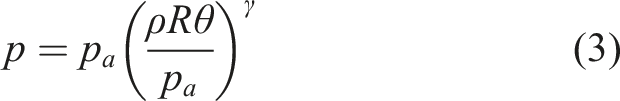
The pressure is related to density and potential temperature through the equation of state for dry air,

p = p_{a} {(\frac{ρ R θ}{p_{a}})}^{γ}

(3)

where p_a = 10⁵ Pa is the reference pressure, R is the specific gas constant for dry air, and γ = c_p/c_v is the ratio of specific heats at constant pressure and constant volume.

2.2. Element-based Galerkin method

We use an element-based Galerkin method for the spatial discretization for the governing equations, following the methodology described in (Giraldo, 1998, 2020). This has been implemented in xNUMA (Kang et al., 2025). In this section, we provide a brief summary of the method and refer readers to (Giraldo, 2020; Kang et al., 2025) for details.

The computational domain $Ω \subset R^{d}$ (d = 3) comprises N_e non-overlapping hexahedral elements Ω_e where $Ω = ⋃_{e = 1}^{N_{e}} Ω_{e}$ . On each element, we represent the solution using nodal values $q_{j}^{(e)} (t)$ and Lagrange basis functions ψ_j( x ) based on Legendre-Gauss-Lobatto (LGL) points:

q_{N} (x, t) = \sum_{j = 1}^{M_{N}} ψ_{j} (x) q_{j}^{(e)} (t),

(4)

with N denoting the polynomial order and M_N = (N + 1)^d nodal points per element. Multiplying the governing equation (2) by the test function ψ_i and integrating over each element yields the continuous Galerkin weak form

\sum_{e = 1}^{N_{e}} \int_{Ω_{e}} ψ_{i} \frac{\partial q_{N}}{\partial t} d Ω_{e} = \sum_{e = 1}^{N_{e}} \int_{Ω_{e}} ψ_{i} S (q_{N}) d Ω_{e} .

(5)

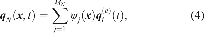
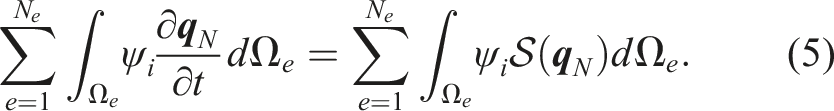
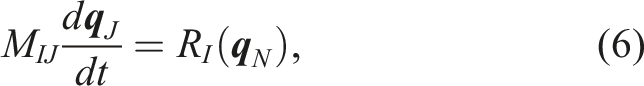
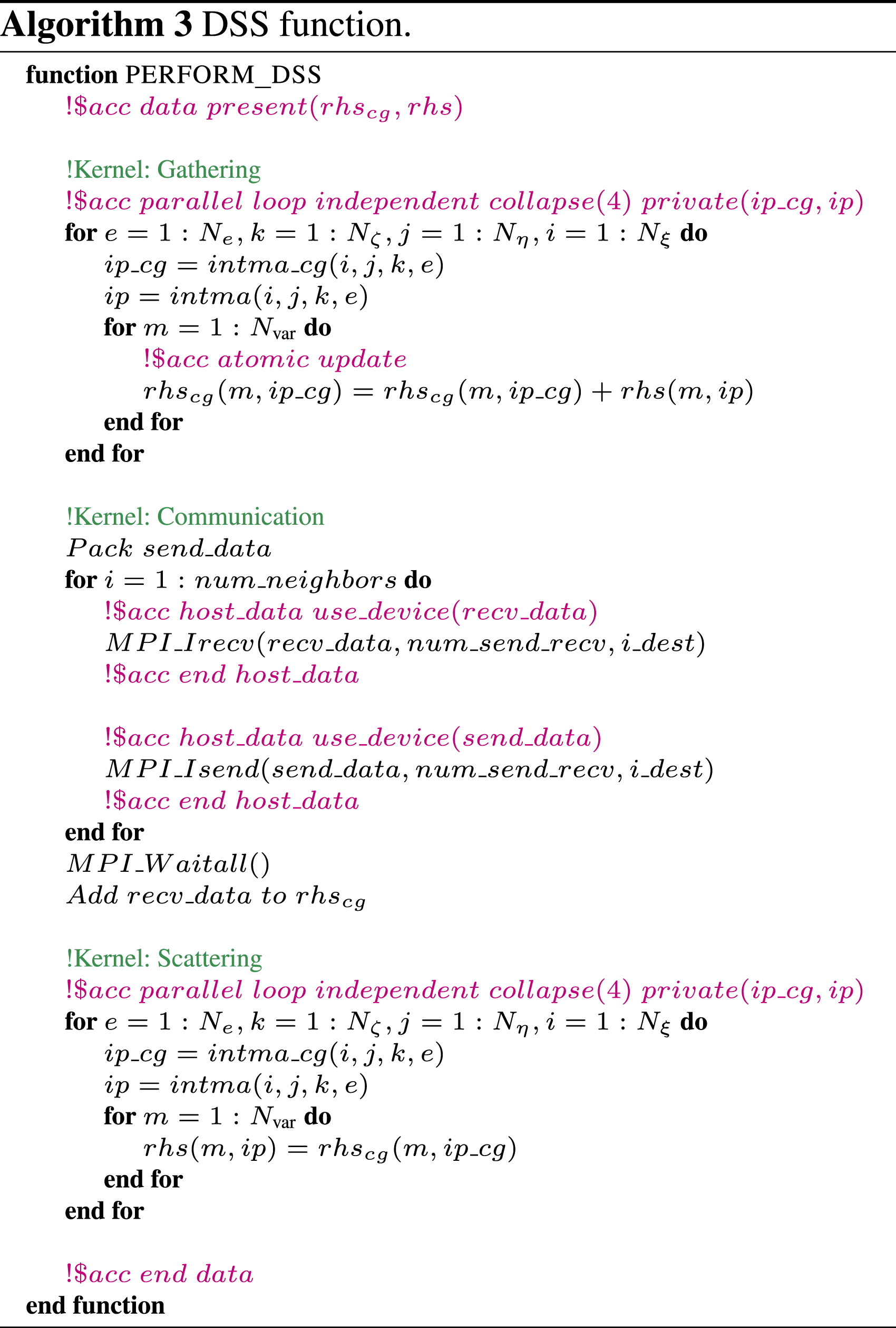
We employ LGL quadrature with collocation (integration points coincide with interpolation nodes), which renders the mass matrix to be diagonal. Global assembly via direct stiffness summation (DSS) (Giraldo, 2020) produces:

M_{I J} \frac{d q_{J}}{d t} = R_{I} (q_{N}),

(6)

where indices

I, J \in \{1, \dots, N_{p}\}

span all N_p global nodes. With the diagonal mass matrix, this simplifies to

\frac{d q_{I}}{d t} = M_{I}^{- 1} R_{I} (q_{N}) .

(7)

2.3. Implicit-explicit (IMEX) time integration

We integrate the semi-discrete equation (7) in time using an implicit-explicit (IMEX) time integrator (Giraldo et al., 2013), which splits the operator $S (q)$ in the governing equations as follows:

\frac{\partial q}{\partial t} = [S (q) - L (q)] + L (q) .

(8)

The terms enclosed in the square bracket represent the slower advective waves and are discretized explicitly. The remaining terms, in the linear operator $L (q)$ , correspond to the fast waves, including acoustic and gravity waves, and are discretized implicitly. This IMEX scheme relaxes the CFL restriction imposed by the fast waves. In this work, we employ the second-order additive Runge-Kutta (ARK2) scheme proposed by (Giraldo et al., 2013), a family of linear multistage schemes. This time integrator has also been used in both (Giraldo et al., 2024; Kang et al., 2025). In (Giraldo et al., 2024), it was referred to as ARK (2,3,2)b and employed within the horizontally explicit vertically implicit (HEVI) formulation, while the same scheme was adopted in (Kang et al., 2025) for the MMF.

The linear system arising from the implicit part of the IMEX formulation is solved using the GMRES Krylov subspace method (Saad and Schultz, 1986) in a fully matrix-free fashion. In this approach, the linearized operator is computed on the fly with no information precomputed or stored. The only memory required is to store the Krylov vectors, which are typically fewer than 20 in the simulations presented.

The complexity of the algorithm is analyzed in our earlier work. Detailed information can be found in our previous paper (Kang et al., 2025).

2.4. Tensor-based hyper-diffusion

We add numerical hyper-diffusion to improve the stability of the numerical scheme. In particular, we implemented a modified form of the original formulation proposed by (Guba et al., 2014), which has also been used in the NUMA model (Giraldo et al., 2024). This modification reduces memory requirements. The hyper-diffusion term is given by

H_{q} = {(- 1)}^{α + 1} {(\nabla \cdot τ \nabla)}^{α} q,

(9)

where q is the state variable, τ is the viscosity tensor, and α is the order. In this work, we employed α = 2, which yields fourth order hyper-diffusion. The viscosity tensor τ is defined through the eigendecomposition as follows:

τ = J E (\begin{matrix} ν_{1} λ_{1}^{- 1} & 0 & 0 \\ 0 & ν_{2} λ_{2}^{- 1} & 0 \\ 0 & 0 & ν_{3} λ_{3}^{- 1} \end{matrix}) {(J E)}^{T},

(10)

where J = ∂ x /∂ ξ denotes the Jacobian matrix of the isoparametric mapping. The viscosity coefficients

(ν_{1}, ν_{2}, ν_{3})

are defined along the principal directions of the metric tensor

G = J^{- 1} J^{- T}

. The tensor G has eigenvalues

(λ_{1}^{- 1}, λ_{2}^{- 1}, λ_{3}^{- 1})

with corresponding normalized eigenvectors ( e ₁, e ₂, e ₃), which forms E . The viscosity parameters ν_i have physical dimensions L²/T^1/α, while kinematic (physical) hyperviscosity ν_p has dimensions L^2α/T. The viscosity parameters can be scaled by the element size Δx and time-step Δt as follows

ν_{i} \equiv {(c_{i})}^{1 / α} \frac{{(Δ x_{i})}^{2}}{{(Δ t)}^{1 / α}} (i = 1, \dots, 3)

(11)

where

c_{i} = (c_{1}, c_{2}, c_{3})

are dimensionless coefficients.

3. GPU implementation

3.1. Base code

The xNUMA code is written in modern Fortran and the base CPU code is parallelized using a Message Passing Interface (MPI) implementation. The simulator utilizes the dynamical core of the nonhydrostatic unified model of the atmosphere, referred to as NUMA (Giraldo et al., 2013; Kelly and Giraldo, 2012). Each simulator object encapsulates the data and functions that define a simulation, including input data, spatial discretization, time integration, and solvers.

The CPU baseline employs MPI for distributed memory parallelism, using element-based domain partitioning where each MPI rank handles a balanced subset of elements (Kang et al., 2025). We chose to keep the grid columns within a partition for potential use of a column-based microphysics model. Inter-rank communication is required for global DSS operations that assemble element contributions across partition boundaries. The multi-GPU implementation extends this parallelization strategy by assigning each GPU to an MPI rank. For detailed descriptions of the CPU implementation, including domain decomposition layouts, computational stencils, and parallel communication patterns, see (Kang et al., 2025; Kelly and Giraldo, 2012).

3.2. OpenACC implementation

In this work, we ported the time integration task, a main component of the simulation, to GPUs using OpenACC directives. Figure 1 illustrates the simulation workflow on the CPU and GPU. Initially, the simulation is set up on the CPUs by reading input parameters, creating the grid, and computing the initial conditions. Subsequently, all data is transferred to GPUs using OpenACC directives to copy data from the CPU to the GPU. On the GPUs, the simulation advances in time by calculating the RHS vector, performing GMRES iterations, and updating the state vector. To output XML outputs and diagnostics, we transfer the GPU value for the state vector to the CPU, again using OpenACC directives. For this work, we have included all data management directives explicitly rather than using NVIDIA compiler implemented unified or managed memory approaches. These latter memory approaches can simplify porting, but can require either code refactoring (managed memory) or bleeding edge software/hardware (unified memory) to function properly. Explicit data management gives us minimal code change requirements while providing the ability to maximize performance.

Figure 1.

Simulation workflow on the CPU and GPU.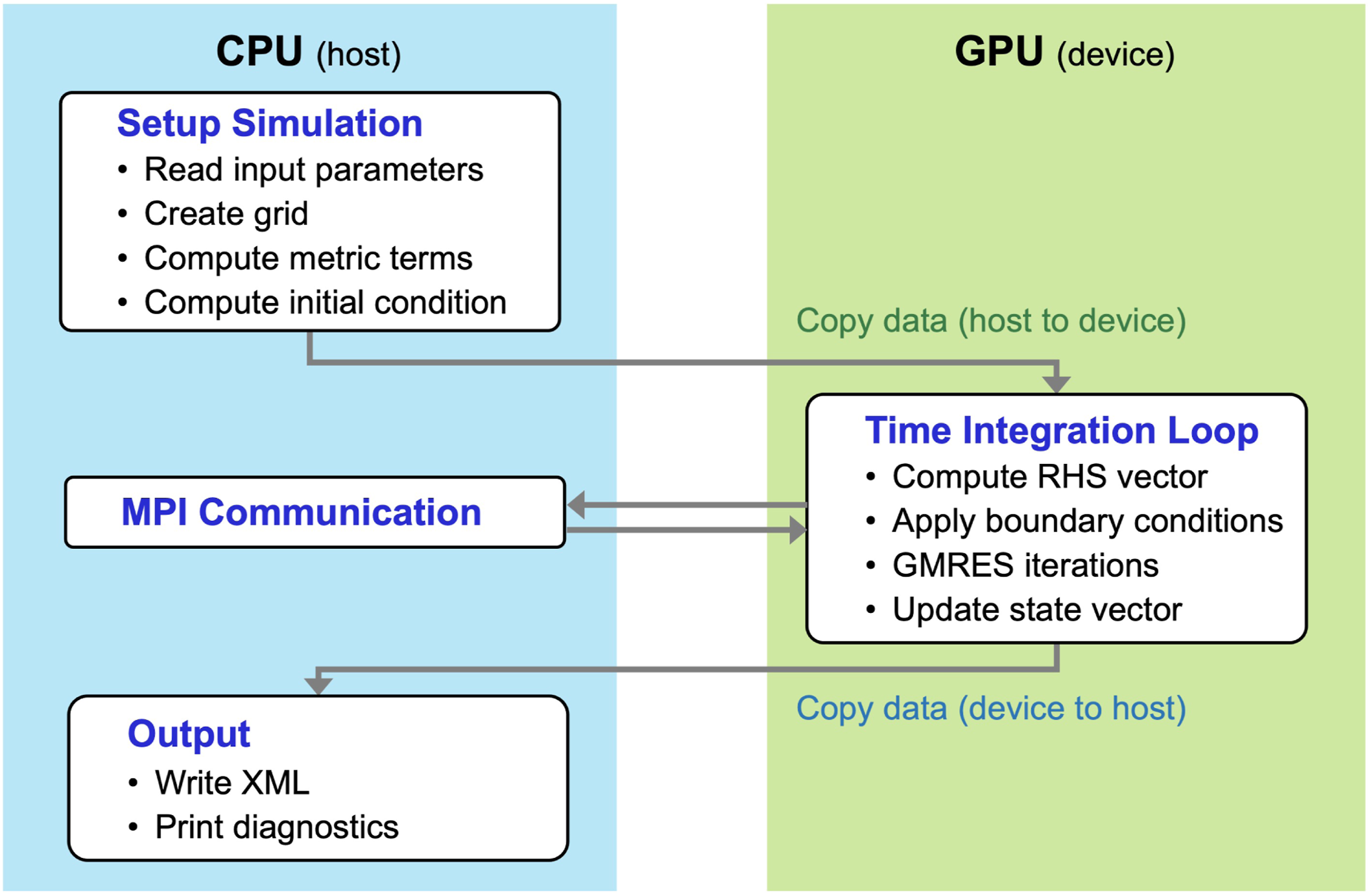

For communication across GPUs, we utilize OpenACC interoperability features that enable MPI communication directly between GPUs. The host_data construct makes GPU data addresses accessible on the CPU, and arrays listed in the use_device clause can be passed to CPU functions. If the hardware does not support CUDA-aware MPI or GPUDirect, standard network communication methods, such as Transmission Control Protocol (TCP), will be used.

To verify the correctness of the GPU implementation, we compared the prognostic variables computed by the CPU-only and GPU-accelerated simulations using PCAST. The results showed agreement within machine precision for all state variables, which confirms the correctness of the OpenACC-based porting.

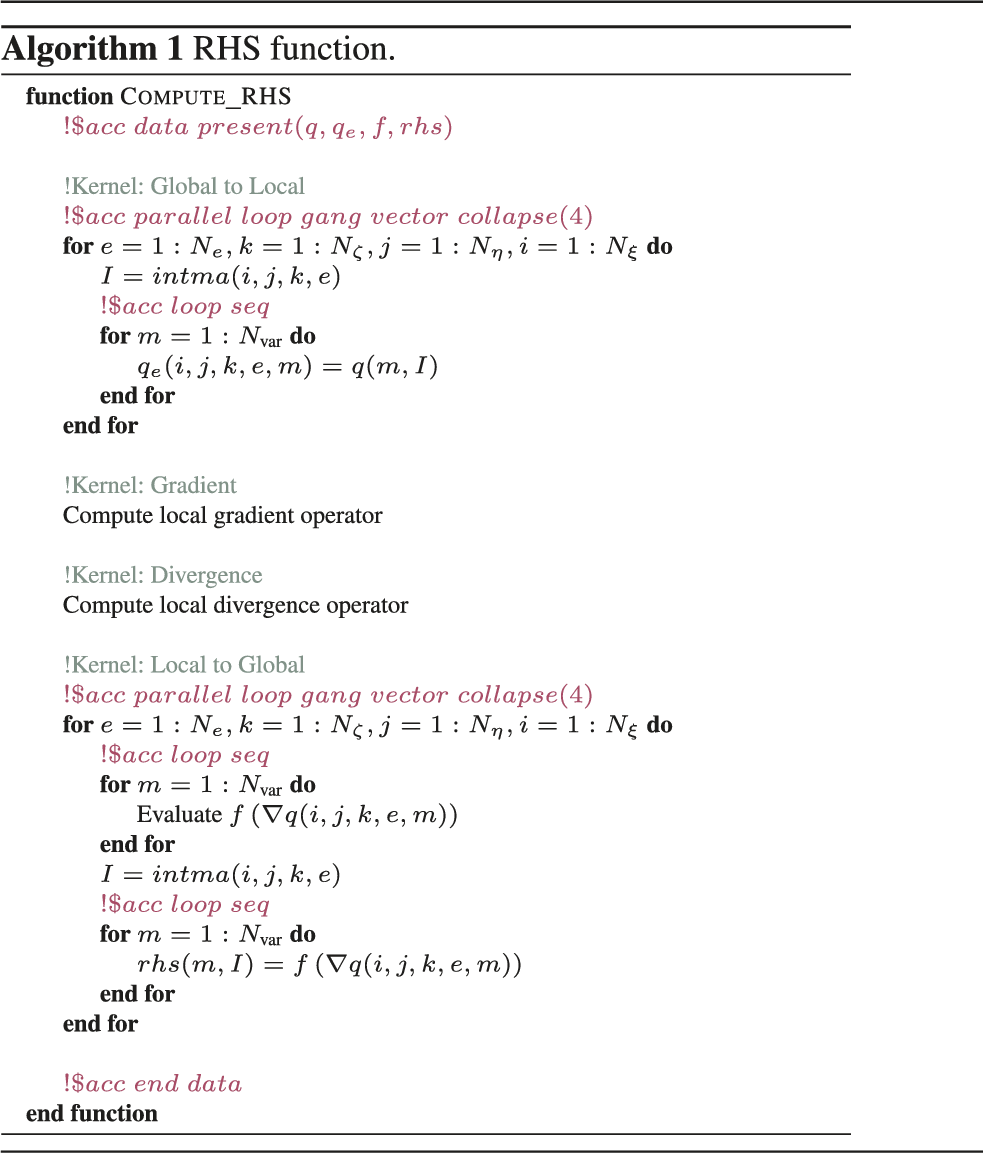
3.3. RHS function

Algorithm 1 presents pseudocode for the function that computes the RHS vector, ported to the GPU using OpenACC directives. In the code, N_e is the number of elements, while N_ξ, N_η, and N_ζ are the number of points within an element in each respective direction. N_var denotes the number of variables at each node. The function intma maps local nodal indices to global nodal indices. The RHS function consists of four kernels: global-to-local, gradient, divergence, and local-to-global kernels. Each kernel is parallelized using the parallel loop directive and optimized with gang and vector elements, which represent coarse-grain and fine-grain levels of parallelism, respectively. Vector parallelism operates within each gang in single instruction multiple threads (SIMT) lanes. The quadruple-nested loops over spectral elements and their nodal points are collapsed into a single loop using the collapse clause, which allows the compiler to maximize parallelism by mapping the nested loop to an unnested parallelizable loop with N_e × N_ζ × N_η × N_ξ independent iterations. Despite also being a parallelizable loop, we found that allowing the innermost loop to run sequentially maximized performance. By parallelizing the outer loops over more contiguous memory indices while sequentializing the largest-stride direction, the memory access pattern becomes more efficient. In addition, the outer loops already provide sufficient parallelism to effectively hide memory latency.

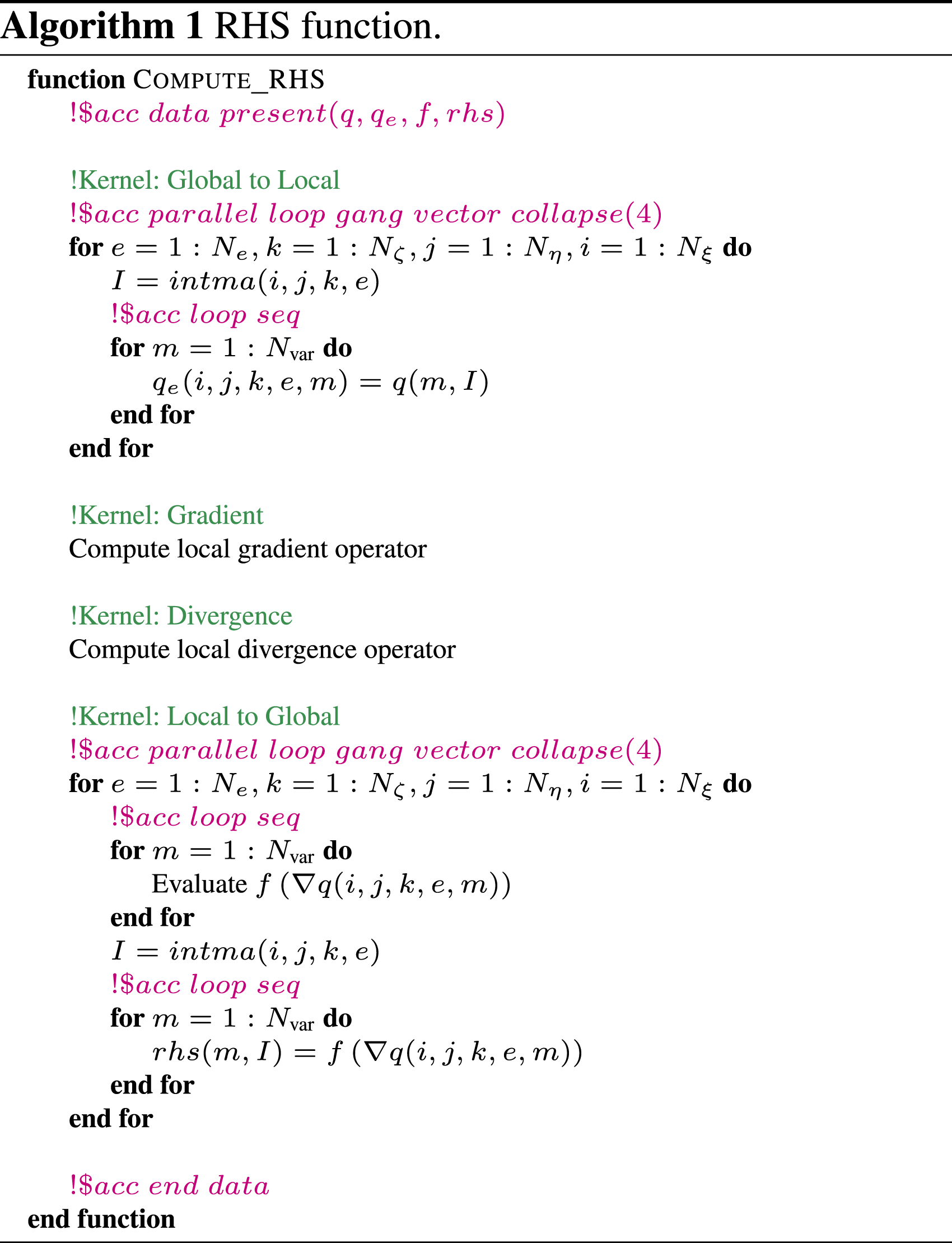
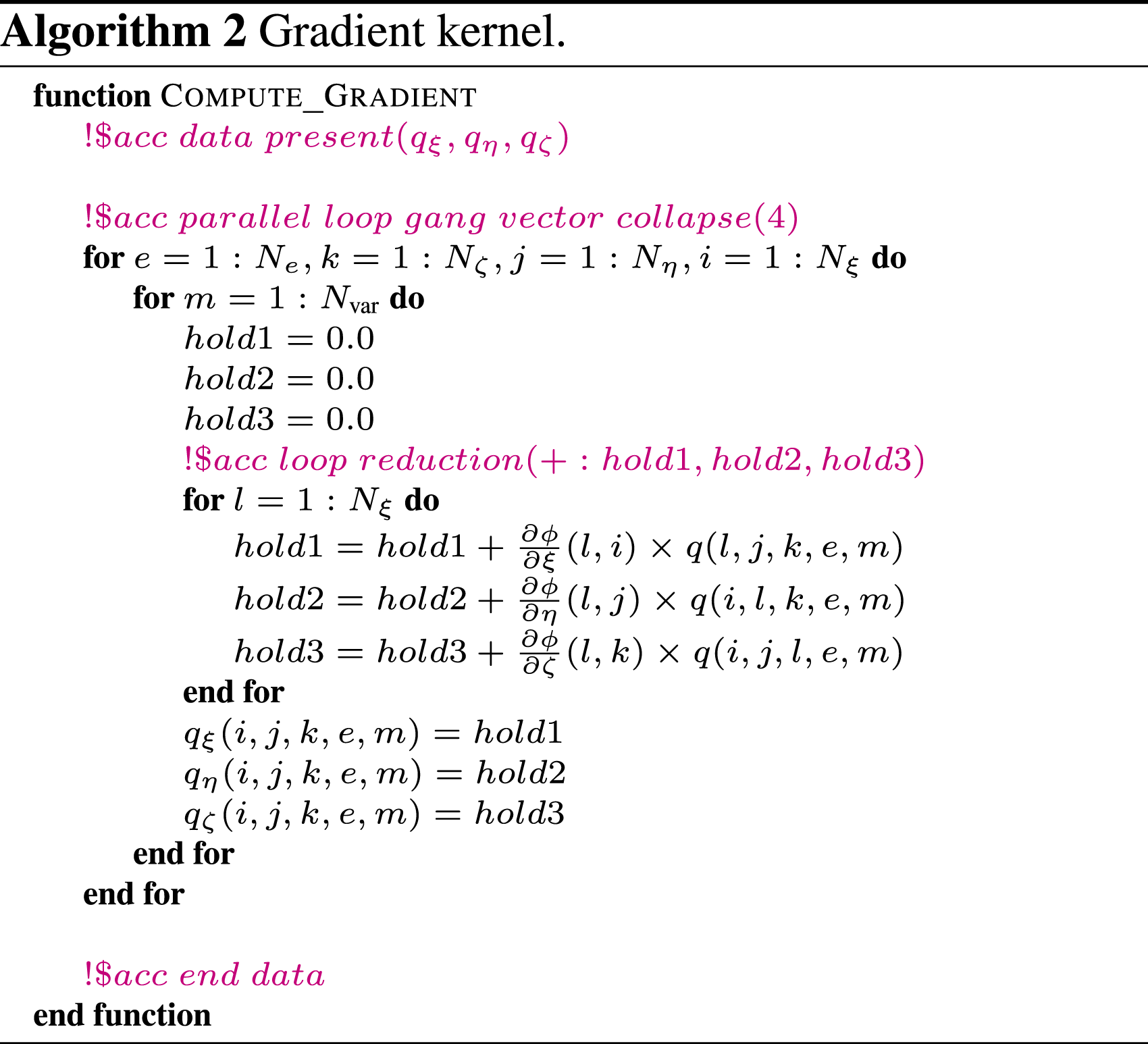
3.4. Gradient kernel

Algorithm 2 presents pseudocode for the function that computes the gradient fields of the prognostic variables. This function is the most computationally intensive part of the code and is executed when evaluating the right-hand side vector or the linearized operator. In the code, q_ξ, q_η, and q_ζ represent the differentiation of the state vector with respect to the reference coordinates, ∂q/∂ξ, ∂q/∂η, and ∂q/∂ζ, respectively.

3.5. Assembly function

Algorithm 3 presents pseudocode for the function that performs the DSS to assemble the global RHS vector. This part of the code requires communication across ranks. The function consists of three major kernels. The first gathering kernels assemble the local RHS vector through overlapping nodes, and therefore requires avoiding race conditions among threads, which is achieved using the atomic update directive. The second kernel exchanges the values of the RHS vector at the grid interface via MPI communications. The host_data directive enables the use of device data within the CPU code, MPI calls in this algorithm, by passing the device address of the data to the CPU. The third kernel scatters the continuous nodal values back to the RHS global array.

4. Simulation setup

4.1. Numerical setup

We simulate a tropical cyclone case using the GPU-accelerated code. The computational domain is a 3D box with horizontal dimensions of 800 km and a vertical height of 20 km, defined as Ω = [−400, 400] × [−400, 400] × [0, 20] km. Doubly periodic boundary conditions are applied at the lateral boundaries, and a no-flux boundary condition is enforced at the bottom surface. To absorb upward gravity waves and prevent reflections, an implicit sponge layer (Kang et al., 2025; Klemp et al., 2008) with a thickness of 4 km is imposed at the top of the domain.

Several values for horizontal grid spacing are tested, with $Δ x \in \{0.5, 1,2,4\}$ km when using fifth-order basis functions (N = 5), while the vertical spacing is fixed at Δz = 167 m. For different orders of the basis function, the grid spacing is adjusted as close as possible to these values. The simulation runs for 6 hours with a time step size of Δt = 0.5 seconds.

The values for the reference variables are taken from the background sounding provided in (Jordan, 1958). Figure 2 presents the profiles of reference potential temperature and reference pressure with respect to height. In the simulation, background wind is not considered.

Figure 2.

Soundings for tropical cyclone simulations: reference potential temperature θ₀ and reference pressure p₀.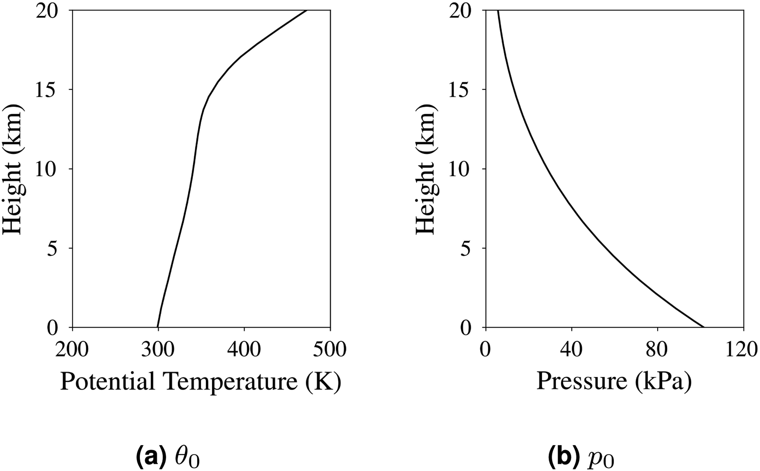

The tropical cyclone is initiated by an idealized vortex used in (Guimond et al., 2016). This vortex is modified from the original form (Nolan et al., 2007; Nolan and Grasso, 2003) to enforce zero velocities at the lateral boundaries. In this vortex, the azimuthal-mean tangential velocity is defined as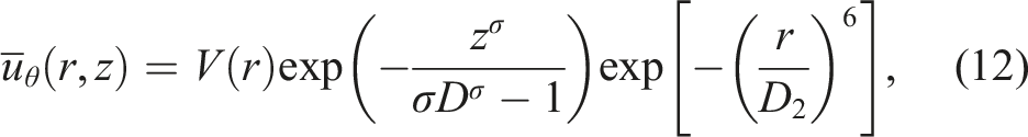

{\bar{u}}_{θ} (r, z) = V (r) \exp (- \frac{z^{σ}}{σ D^{σ} - 1}) \exp [- {(\frac{r}{D_{2}})}^{6}],

(12)

where V is the surface tangential velocity, σ = 2, D₁ = 5823 m, and D₂ = 200 km. The surface tangential velocity is calculated by integrating a Gaussian distribution of vorticity with a peak of 1.5 × 10⁻³ s⁻¹ at the vortex center, and a maximum wind speed of 21.5 m/s at a radius of 50 km.

The RI of tropical cyclones is driven by the vortex response to latent heating injected into the boundary layer. In this research, we incorporate the observational latent heating into the source term S_θ in Eq. 1c. A time-varying 3D observational heating profile was obtained from airborne Doppler radar measurements during the RI of Hurricane Guillermo (1997) (Hasan et al., 2022). Figure 3 presents snapshots of the asymmetric spatial distribution of latent heating at different time points. Over the duration of 6 hours, 11 sampling points of latent heating are used to interpolate the heating source term.

Figure 3.

Latent heating in the region [−60, 60] × [−60, 60] × [0, 20] km.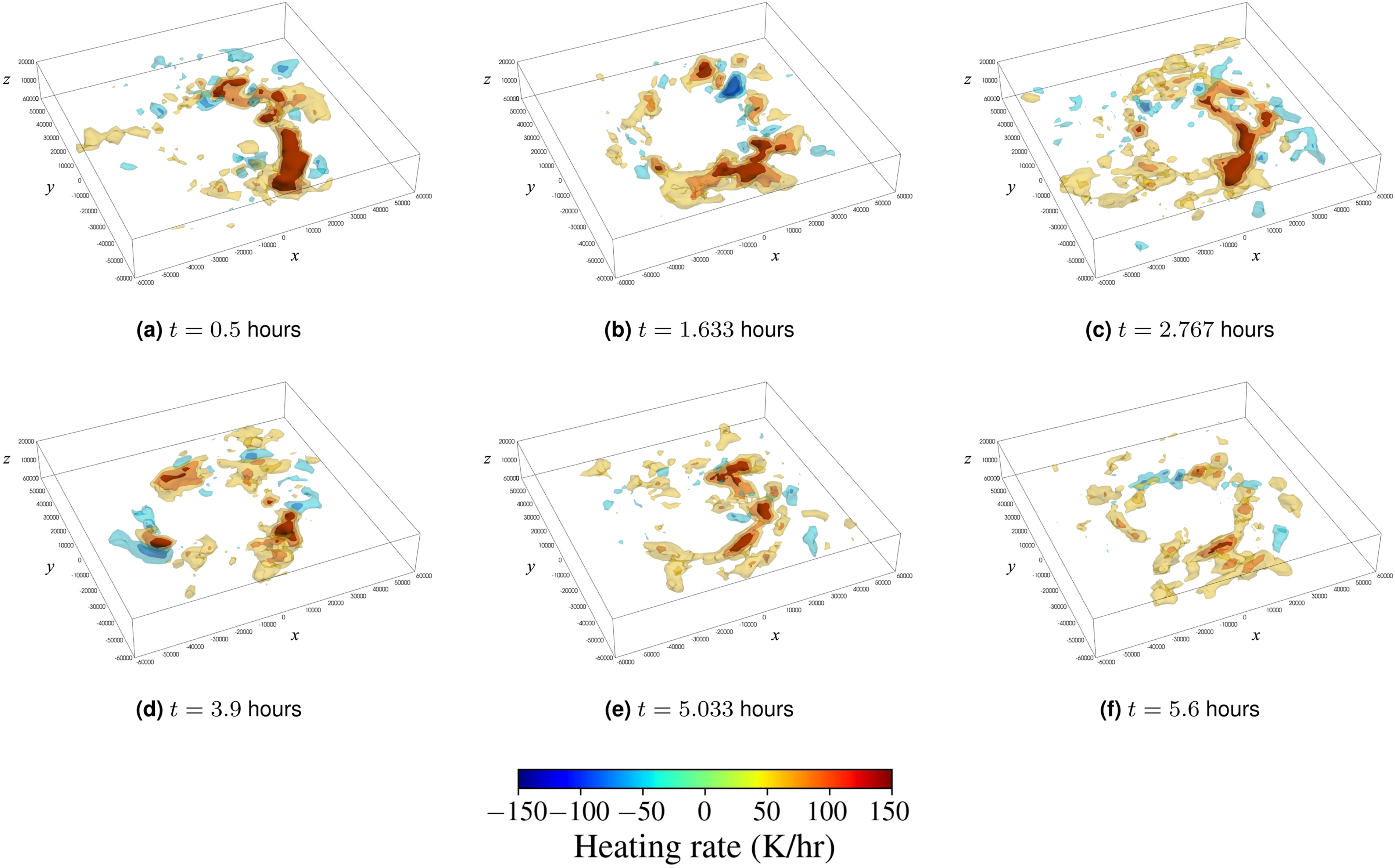

4.2. Computing system

The performance of the GPU code for tropical cyclone simulations is evaluated on the Delta system, which was ranked No. 100 in the November 2025 TOP 500 list (top500.org, 2025). Delta is an advanced computing resource maintained by the National Center for Supercomputing Applications (NCSA) at the University of Illinois, and supported by the National Science Foundation (NSF). While Delta provides access to NVIDIA A100 and H200 GPUs, we only use A100 GPUs for performance tests in this study. Delta features 100 A100 GPU nodes, and each node is equipped with 64 AMD EPYC 7763 (Milan) CPUs and 4 A100 GPUs. The compute nodes are connected via a low-latency high-bandwidth HPE/Cray Slingshot interconnect.

The parallel code is compiled using NVIDIA HPC compilers (version 22.5), which include OpenMPI compiler wrappers. All performance tests in this study are conducted using double-precision calculations.

5. Numerical results and performance analysis

5.1. Numerical results

Figures 4 and 5 show the velocity magnitude and potential temperature perturbation, respectively, on the y-z plane at the center of the domain. In the initial state at t = 0 hours, a single idealized vortex defined by equation (12) is located at the center near the surface, with no thermal perturbation. By injecting thermal energy into the dynamical system, a strong updraft develops in the eyewall and leads to asymmetric and complex vortex structures. Figure 6 shows the vortical structures in the eye and spiral bands of the tropical cyclone at t = 6 hours.

Figure 4.

Velocity magnitude at the middle y-z plane. (The domain is vertically stretched by a factor of 10 for visual purposes).

Figure 5.

Potential temperature perturbation at the middle y-z plane. (The domain is vertically stretched by a factor of 10 for visual purposes).

Figure 6.

Vortical structures in the eye and spiral bands of the tropical cyclone at t = 6 hours. (Vortices are visualized using the Q-criterion).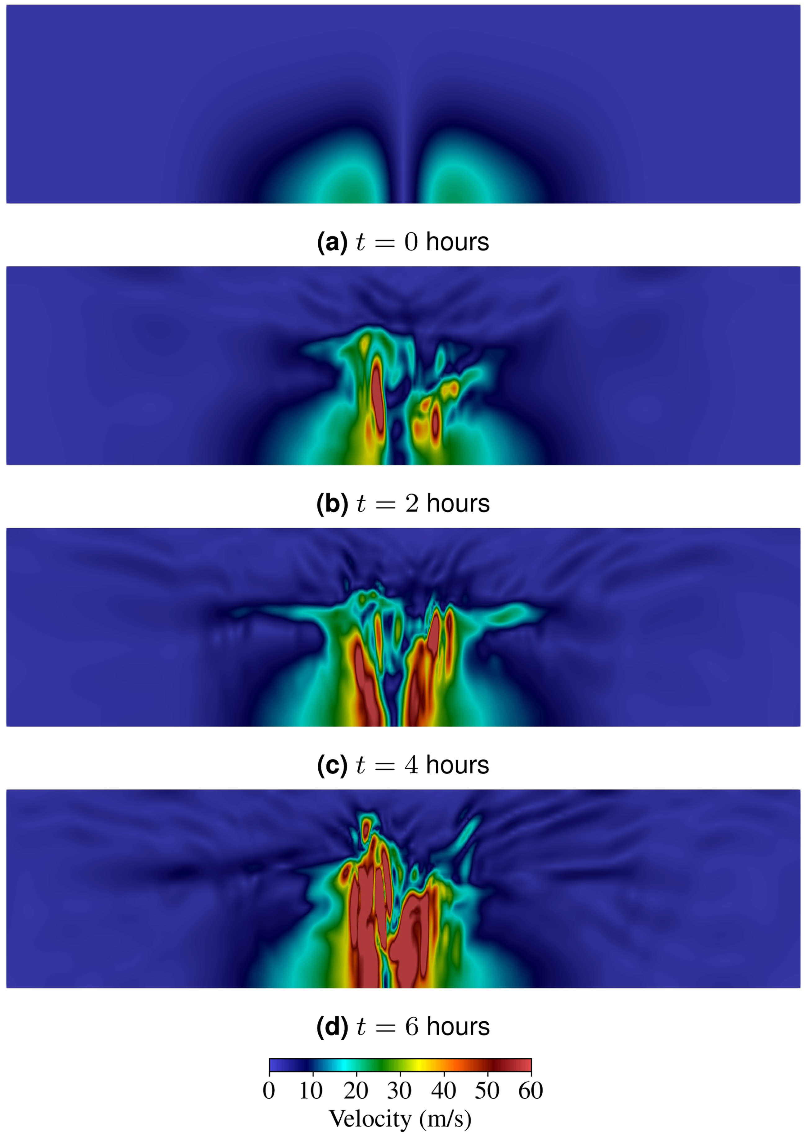

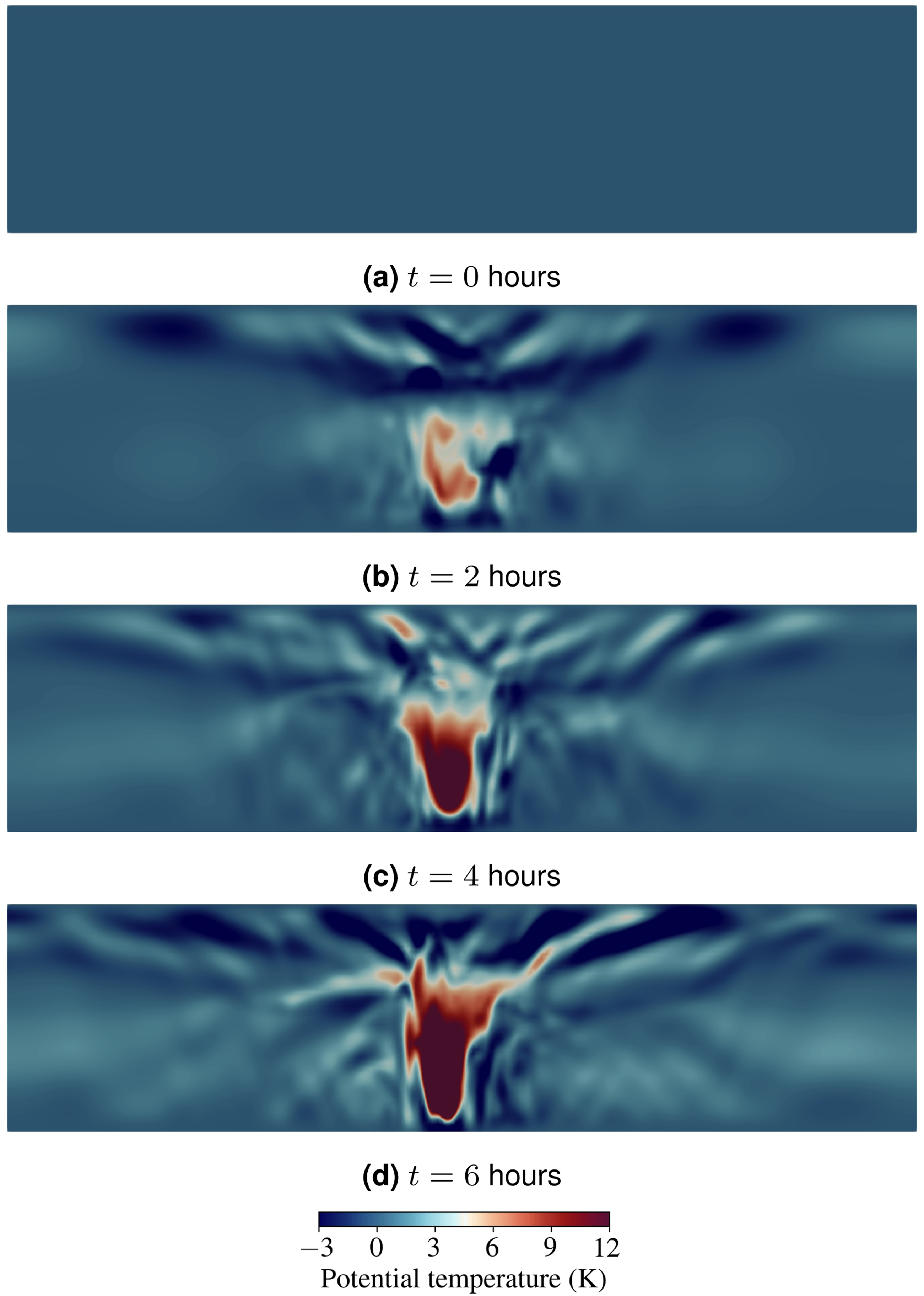
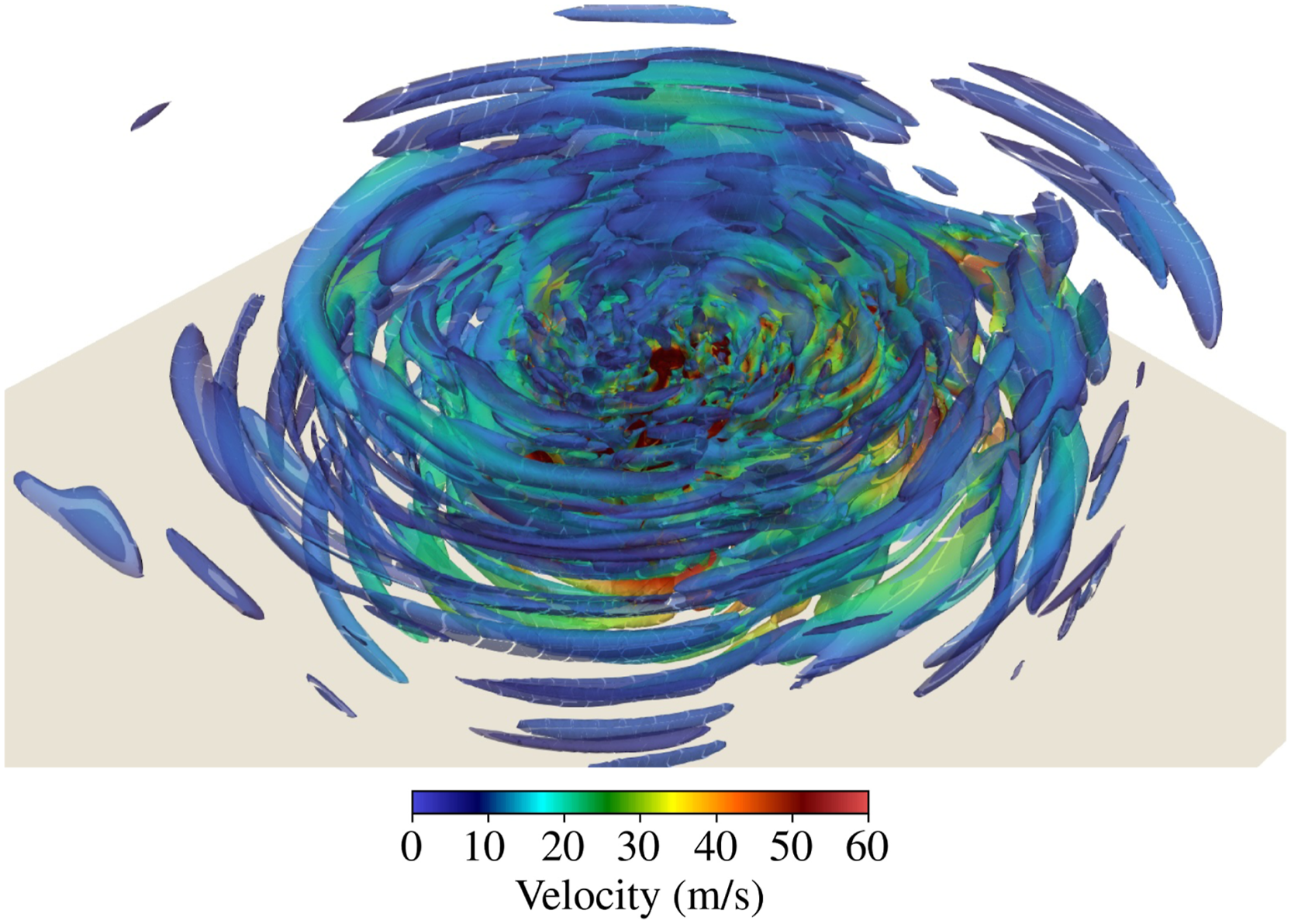
Figure 7 shows the velocity magnitude on the horizontal plane at various heights. Uneven temperature distribution near the surface significantly contributes to the asymmetric structure of the tropical cyclone, where the extent of asymmetry varies with height.

Figure 7.

Velocity magnitude at t = 6 hours in the horizontal region [−20, 20] × [−20, 20] km at various heights.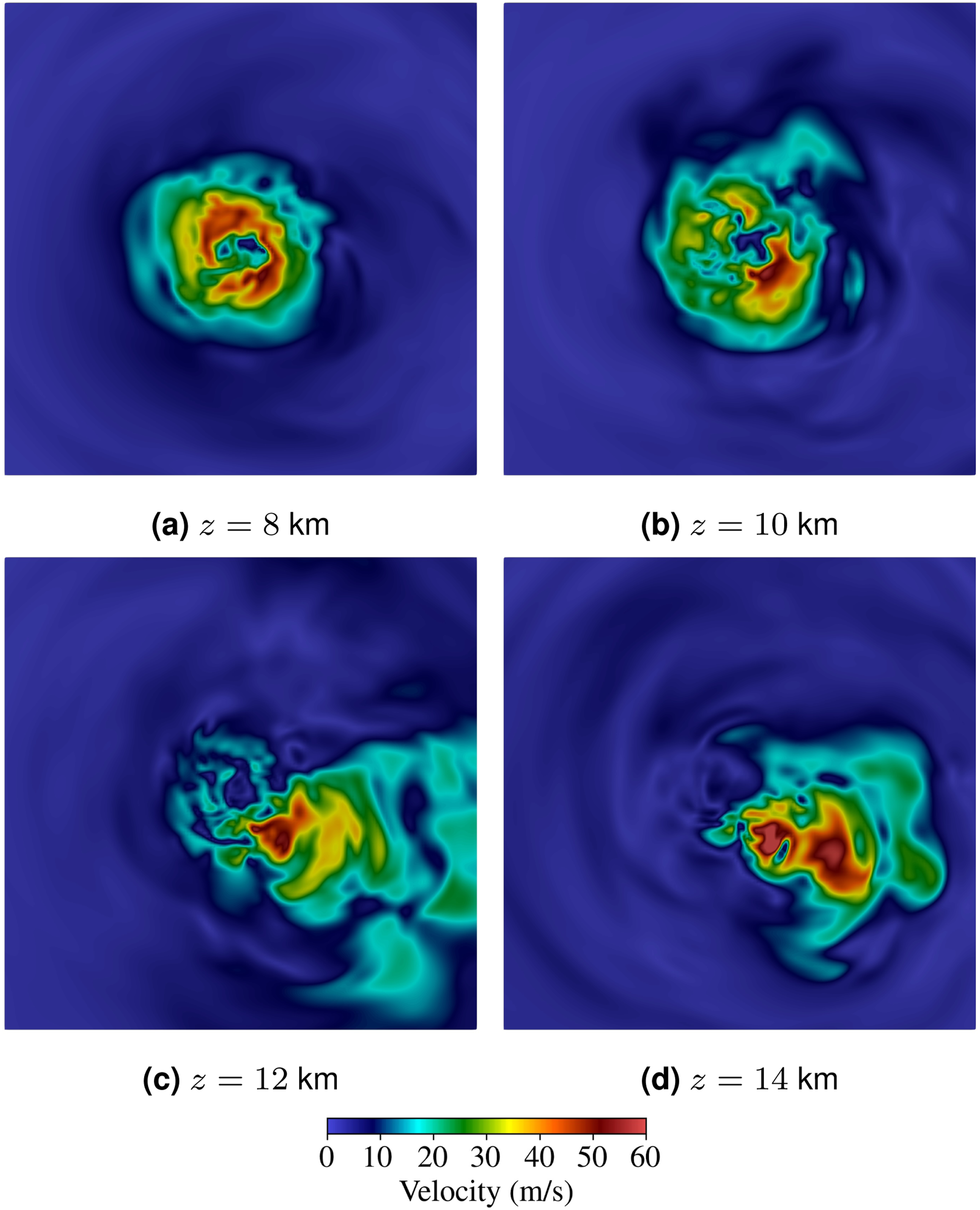

In order to quantify the magnitude of the vortex, we use the index of maximum tangential velocity and denote it as the RI velocity. In this work, the RI velocity is defined as the maximum of azimuthal-averaged tangential velocity as follows:

u_{RI} = \max ({\bar{u}}_{θ} (r, z)),

(13)

where.

\begin{align} {\bar{u}}_{θ} (r, z) & = \frac{1}{2 π} \int_{0}^{2 π} u_{θ} (r, θ, z) d θ \end{align}

(14)

\begin{align} u_{θ} & = ‖ u_{θ} ‖ \end{align}

(15)

\begin{align} u_{θ} & = (I - e_{r} \otimes e_{r} - e_{z} \otimes e_{z}) u . \end{align}

(16)

Here, e _r and e _z are the unit vectors in the radial and vertical directions, respectively, which are calculated as e _r = r /| r |, r = (x − x_c, y − y_c, 0), and e _z = (0, 0, 1). The vertically varying centroid of the TC, x _c = (x_c, y_c, z), is estimated as the weighted center of the velocity magnitude field:

x_{c} = \frac{\int_{x} \int_{y} | u | x d x d y}{\int_{x} \int_{y} | u | d x d y},

(17)

where L_x and L_y are the lengths of the domain along the x and y directions, respectively.

We propose a simplified calculation of azimuthally-averaged velocity, as given in equation (14). The azimuthally-averaged velocity is approximated as the arithmetic mean of points that fall within a narrow circular strip at each radial distance r_i and height z_i. This circular strip is defined as $Ω_{strip} (r_{i}, z_{i}) = \{(r, θ, z) ∣ r_{i} - \frac{ε}{2} < r < r_{i} + \frac{ε}{2}, 0 \leq θ \leq 2 π, z = z_{i}\}$ , where ɛ is the width of the strip. The averaged tangential velocity is evaluated as

{\bar{u}}_{θ} (r, z) \approx \frac{1}{N_{p}} \sum_{i = 1}^{N_{p}} u_{θ} (r_{i}, θ_{i}, z_{i}), for (r_{i}, θ_{i}, z_{i}) \in Ω_{strip} (r, z),

(18)

where N_p is the number of points that belong to the strip.

Figure 8 presents the time evolution of the RI velocity at various grid resolutions, together with the maximum horizontal velocity. The RI velocity is calculated using 50 equi-width strips to average the tangential velocity. At all grid resolutions, the RI velocity exhibits a significant increase exceeding 20 m/s from its initial state. This is higher than the typical RI threshold of 13 m/s, which indicates that the occurrence of the RI event is effectively captured. The RI velocity produces a similar curve across all the resolutions and converges when the grid resolution is finer than Δx = 2 km, whereas, the maximum horizontal velocity shows larger variance between the profiles of different resolutions.

Figure 8.

Maximum horizontal velocity (u_max) and RI velocity (u_RI) at resolutions 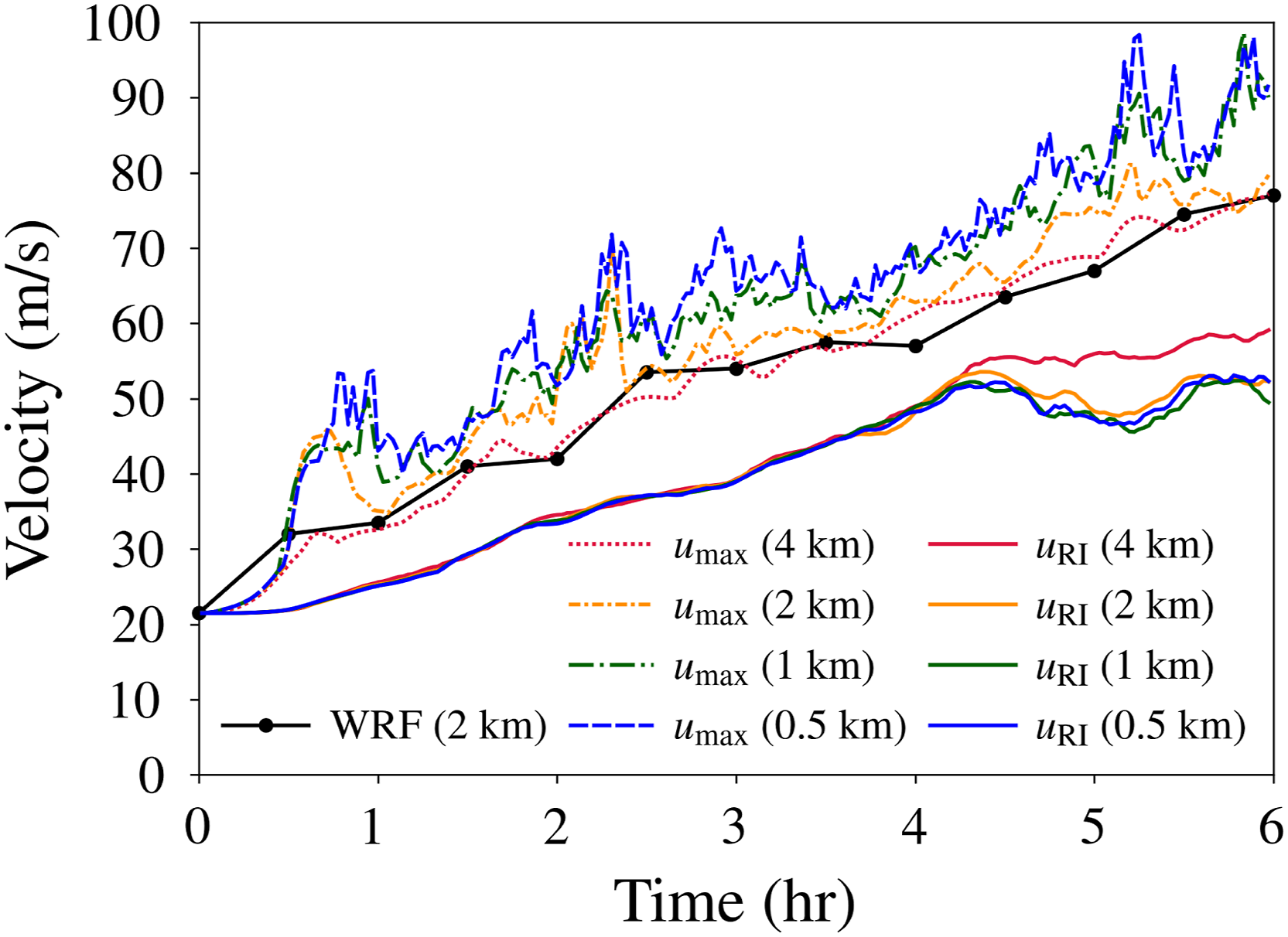$Δ x = \{0.5, 1,2,4\}$ km.

The maximum horizontal velocity results are compared with those obtained using the Weather Research and Forecasting (WRF) model with reduced eddy viscosity and a horizontal grid spacing of 2 km (Hasan et al., 2022). The resulting time series show good agreement between the two models, which validates the present simulation results.

5.2 Speedup and energy consumption

The execution time and energy consumption are compared between a CPU-based simulation using 128 AMD and 4 A100 processors. The test grid consists of 80 × 80 × 24 fifth-order elements, which results in 165,888,000 degrees of freedom (DOFs). Table 1 summarizes the comparison between the two simulations. The maximum power consumptions are assumed based on the hardware specifications.

Table 1.

Comparison of total energy consumption during 100 time steps between CPUs (AMD EPYC 7763) and GPUs (NVIDIA A100).

	CPU	GPU
Max. Power consumption (W)	280 (per node)	400 (per GPU)
Number of nodes	2	1
Number of processors	128	4
Execution time per step (seconds)	5.563	0.536
Energy consumption per step (J)	3115.3	857.6

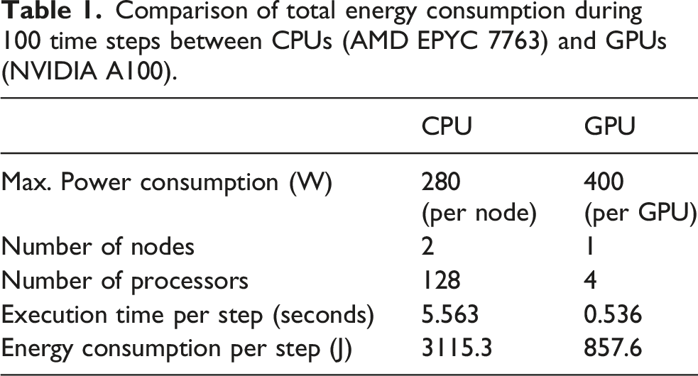
Execution times are measured for the time integration loop, i.e., after the simulation setup stage in Figure 1, over 100 time steps from the initial state. The CPU run employs the base code, originally optimized for CPUs. The GPU-accelerated code achieves approximately 10.4× speedup over the CPU code for the current configuration. This speedup is likely due to the higher FLOP capacity of the GPU and reduced communication overhead from the smaller number of processors.

The energy consumption per time step in the GPU simulation is approximately 3.63× lower than that of the CPU simulation. Although a single GPU consumes more power than a single CPU node, the total energy consumption is significantly reduced in the GPU run due to 10.4× speedup. This indicates that the GPU implementation offers greater energy efficiency compared to the purely CPU-based approach. To emphasize this point, Table 1 shows that 4 GPUs are 3.63× more efficient than 128 CPUs; therefore, we require 128/4 × 3.63 ≈ 116 CPUs to match a single GPU. To perform equivalent simulations that we performed on 256 GPUs would require nearly 30,000 CPUs (approximately 4.5× the CPU capacity of Delta).

5.3. Scalability

To evaluate the scalability of the GPU implementation, we measure the strong and weak scaling performance.

Figure 9 shows the strong scaling of the GPU implementation. The grid is composed of 160 × 160 × 24 fifth-order elements, which results in a total of 663,552,000 DOFs. Strong scalability tends to degrade as the number of GPUs increases. This can be attributed to increased GPU memory access latency, and its effects become relatively more significant as each rank holds a smaller portion of the problem. It is noteworthy that GPUs are the most performant when they are fully saturated.

Figure 9.

Strong scaling of the GPU implementation.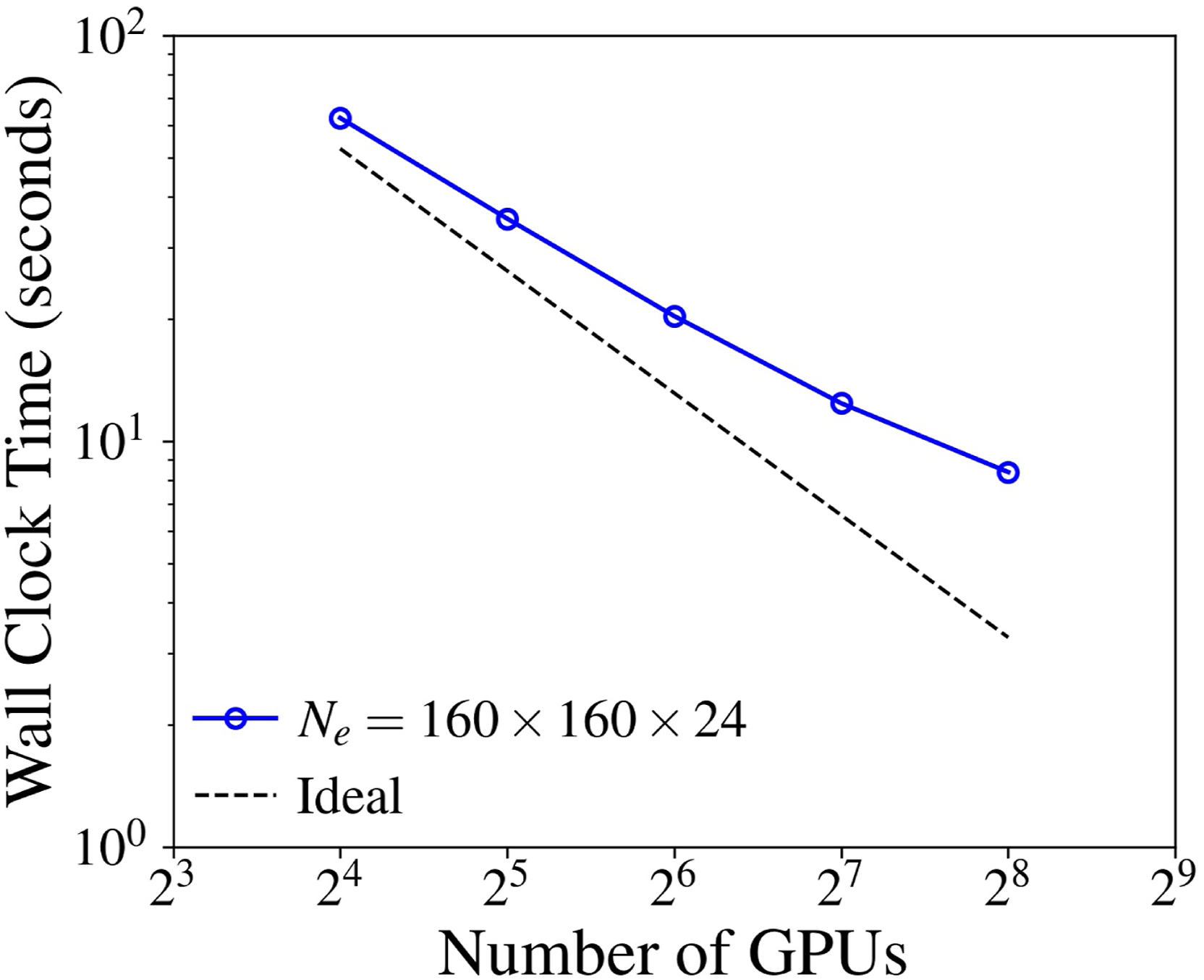

For weak scaling, the grid size is increased proportionally to the number of GPUs. To achieve this, the grid resolution is doubled while keeping the number of elements per GPU at 40 × 40 × 24 (41,472,000 DOFs), and the temporal resolution constant at Δt = 0.5 seconds (the largest problem shown has 5.31 billion DOFs). The order of basis function is N = 5 in all direction. Figure 10 shows the wall clock time per time step for the weak scaling test. The execution time converges as the number of GPUs increases. This trend arises because larger problem sizes require more GMRES iterations for the implicit solve. In this work, the maximum number of GMRES iterations is limited to 20. This result highlights the high performance and scalability of the code.

Figure 10.

Weak scaling of the GPU implementation.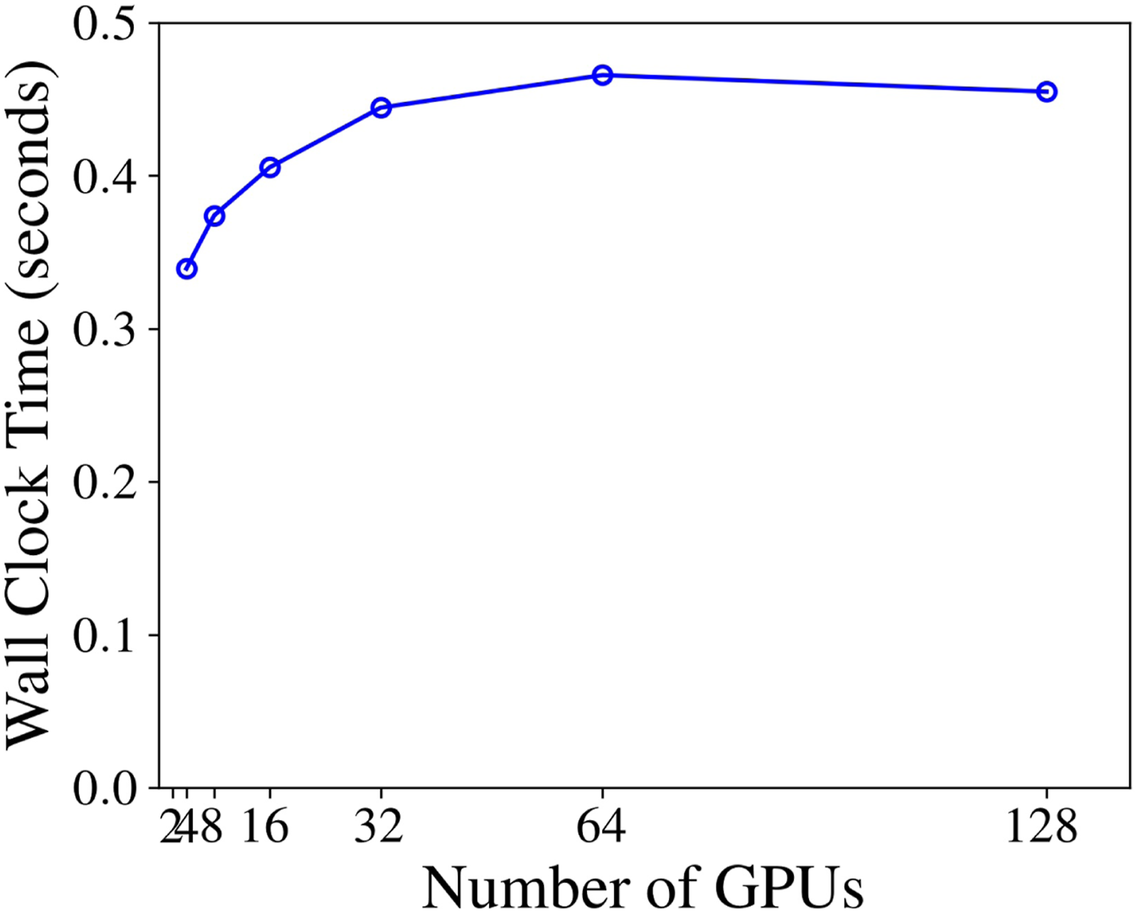

5.4. Kernel performance

We evaluate the performance of the main kernels to compute the RHS vector in Algorithm 1 using the roofline model (Williams et al., 2009). While both gradient and divergence operators are also invoked within the Laplacian subroutine in the code, our analysis focuses on these kernels within the RHS routine. The roofline model uses the metrics of double-precision floating point operations rates in GFLOPS/s, bandwidth in GB/s, and the arithmetic intensity (GFLOPS/GB). The measured peak performance and bandwidth of NVIDIA A100 GPUs in the test are 7329 GFLOPS/s and 1506 GB/s, respectively.

Figure 11 shows the GFLOP/s performance, arithmetic intensity, and roofline plots for various orders of the basis function, where the number of DOFs is held constant. The gradient and divergence kernels are computationally intensive and achieve higher performance as the order of the basis function increases. The measured performance for the gradient kernel ranges from 9.5% to 12.3% of the peak performance, while the divergence kernel achieves between 4.1% and 6.2%. In the gradient kernel presented in Algorithm 2, we fused the three innermost loops corresponding to the differentiation matrix multiplications in the ξ-, η-, and ζ-directions into a single loop. This optimization reduces global memory accesses and improves register reuse by reusing the q array for the state vector within the same thread. In contrast, the divergence kernel launches separate loops for each differentiation operation, which results in lower performance; however, it accounts for only a small fraction of the total runtime.

Figure 11.

GFLOP/s performance, arithmetic intensity, and roofline model for four main kernels in the RHS function.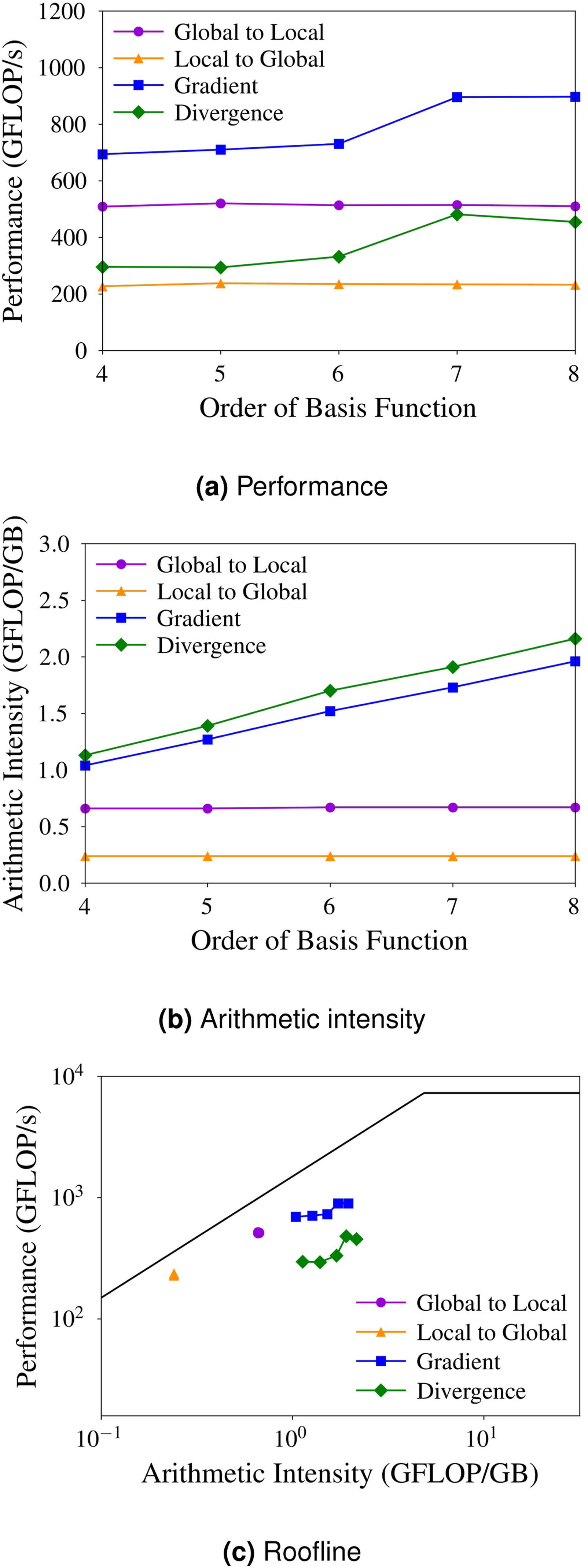

The higher-order basis functions result in greater arithmetic intensity and consequently higher performance, as shown in Figure 11. This implies the potential of high-order methods to better exploit GPUs capabilities. In contrast, the performance of the global-to-local and local-to-global kernels remain independent of the basis function order, 7.1% and 3.2% of the peak performance, respectively, as they simply loop over the grid points and their associated DOFs.

6. Conclusions

In this work, we ported the nonhydrostatic atmospheric model xNUMA to GPUs using the OpenACC programming model. This approach facilitates simple maintenance of the code. The entire time-integration process, including implicit and explicit steps, is performed on the GPU. A matrix-free implementation of the implicit solution is well-suited for GPU computations.

The model successfully simulates realistic tropical cyclones on GPUs and captures the RI process. The simplified calculation of azimuthally-averaged velocity yields converged results of RI across various horizontal grid spacings.

The GPU-accelerated code yields an energy-efficient simulation, achieving a 3.63× improvement over the CPU version. The GPU implementation demonstrates both strong and weak scaling, as well as efficient kernel performance on NVIDIA A100 GPUs. We expect that this research will help accelerate high-fidelity simulations for numerical weather prediction.

Our future work includes the following:

• Using the initial state obtained from observational data to produce more realistic tropical cyclones.

• Adding a precipitation microphysics model to simulate moist dynamics of tropical cyclones.

• Accelerating the multiscale modeling framework (Kang et al., 2025) using GPUs.

• Developing an efficient and GPU-portable preconditioner for the implicit solver.

Footnotes

Acknowledgements

The authors gratefully acknowledge the help and support from Dave Norton (NVIDIA) for helping us get started on this path. This work was supported by the Office of Naval Research under Grant No. N0001419WX00721. F. X. Giraldo was also supported by the National Science Foundation under grant AGS-1835881. This work was performed when Soonpil Kang held a National Academy of Sciences’ National Research Council Fellowship at the Naval Postgraduate School. Part of Soonpil Kang’s work was performed under the auspices of the U.S. Department of Energy by Lawrence Livermore National Laboratory under Contract DE-AC52-07NA27344. LLNL-JRNL-2004409. This work used Delta at the National Center for Supercomputing Applications (NCSA) through allocation MTH240030 from the Advanced Cyberinfrastructure Coordination Ecosystem: Services & Support (ACCESS) program, which is supported by National Science Foundation (NSF).

ORCID iD

Soonpil Kang

Funding

The authors disclosed receipt of the following financial support for the research, authorship, and/or publication of this article: National Centre for Supercomputing Applications; MTH240030; Lawrence Livermore National Laboratory; DE-AC52-07NA27344; National Science Foundation; AGS-1835881; Office of Naval Research; N0001419WX00721.

Declaration of conflicting interests

The authors declared no potential conflicts of interest with respect to the research, authorship, and/or publication of this article.

Author biographies

Soonpil Kang is a postdoctoral researcher in the Atmospheric, Earth, and Energy Division at Lawrence Livermore National Laboratory. Prior to this, he was a postdoctoral researcher in the Department of Applied Mathematics at the Naval Postgraduate School. He received his Ph.D. in Civil Engineering from the Univeristy of Illinoist at Urbana-Champaign. His research focuses on computational modeling and scientific computing for multiphysics problems—including atmospheric modeling and fluid-structure interaction—and implementing these methods on high-performance computing systems.

Francis X. Giraldo is a distinguished professor in the Department of Applied Mathematics and holds a joint appointment in the Department of Mechanical and Aerospace Engineering at the Naval Postgraduate School in Monterey California; He also holds an appointment as adjunct professor in the Department of Applied Mathematics at the University of California at Santa Cruz. He received degrees from Princeton and the University of Virginia and pioneered element-based Galerkin methods in nonhydrostatic atmospheric modeling and through his teaching and collaboration has helped a number of atmospheric modeling efforts develop operational weather predictions systems based on these methods. His book on element-based Galerkin methods was published by Springer in 2020. His research is primarily focused on applied problems in climate, weather, and ocean.

Seth Camp is a Senior Applications Engineer at NVIDIA working in the NVHPC Compiler Group. He earned undergraduate degrees in Math and Physics from Berry College and a Ph.D. in Physics from Louisiana State University. He has previously worked with the Naval Research Laboratory on their Ocean Modeling and Global Ocean Forecasting team, focusing on computational efficiency of large legacy parallel Fortran applications and spends a lot of his time helping international weather forecasting groups port their codes to run on GPUs.

References

Abdi

Giraldo

Constantinescu

, et al. (2019a) Acceleration of the IMplicit–EXplicit nonhydrostatic unified model of the atmosphere on manycore processors. The International Journal of High Performance Computing Applications 33(2): 242–267. Available at: https://doi.org/10.1177/1094342017732395

Abdi

Wilcox

Warburton

, et al. (2019b) A GPU-Accelerated continuous and discontinuous Galerkin non-hydrostatic atmospheric model. The International Journal of High Performance Computing Applications 33(1): 81–109. Available at: https://doi.org/10.1177/1094342017694427

Andrej

Atallah

Bäcker

J-P

, et al. (2024) High-performance finite elements with MFEM. The International Journal of High Performance Computing Applications: 10943420241261981. https://doi.org/10.1177/10943420241261981

Fischer

Tang

Corbosiero

(2019) A climatological analysis of tropical cyclone rapid intensification in environments of upper-tropospheric troughs. Monthly Weather Review 147(10): 3693–3719. https://doi.org/10.1175/mwr-d-19-0013.1

Fischer

Kerkemeier

Min

, et al. (2022) NekRS, a GPU-Accelerated spectral element Navier–Stokes solver. Parallel Computing 114: 102982. Available at: https://doi.org/10.1016/j.parco.2022.102982

Giraldo

(1998) The Lagrange–Galerkin spectral element method on unstructured quadrilateral grids. Journal of Computational Physics 147(1): 114–146. Available at: https://doi.org/10.1006/jcph.1998.6078

Giraldo

(2020) An Introduction to Element-based Galerkin Methods on tensor-product Bases: Analysis, Algorithms, and Applications. Springer Nature.

Giraldo

Restelli

Läuter

(2010) Semi-implicit formulations of the Navier–Stokes equations: application to nonhydrostatic atmospheric modeling. SIAM Journal on Scientific Computing 32(6): 3394–3425. Available at: https://doi.org/10.1137/090775889

Giraldo

Kelly

Constantinescu

(2013) Implicit-explicit formulations of a three-dimensional nonhydrostatic unified model of the atmosphere (NUMA). SIAM Journal on Scientific Computing 35(5): B1162–B1194. https://doi.org/10.1137/120876034

10.

Giraldo

de Bragança Alves

FAV

Kelly

, et al. (2024) A performance study of horizontally explicit vertically implicit (HEVI) time-integrators for non-hydrostatic atmospheric models. Journal of Computational Physics 515: 113275. https://doi.org/10.1016/j.jcp.2024.113275

11.

Guba

Taylor

Ullrich

, et al. (2014) The spectral element method (SEM) on variable-resolution grids: evaluating grid sensitivity and resolution-aware numerical viscosity. Geoscientific Model Development 7(6): 2803–2816. https://doi.org/10.5194/gmd-7-2803-2014

12.

Guimond

Reisner

Marras

, et al. (2016) The impacts of dry dynamic cores on asymmetric hurricane intensification. Journal of the Atmospheric Sciences 73(12): 4661–4684. https://doi.org/10.1175/jas-d-16-0055.1

13.

Hasan

Guimond

, et al. (2022) The effects of numerical dissipation on hurricane rapid intensification with observational heating. Journal of Advances in Modeling Earth Systems 14(8): e2021MS002897. https://doi.org/10.1029/2021ms002897

14.

Jordan

(1958) Mean soundings for the west indies area. Journal of the Atmospheric Sciences 15(1): 91–97. https://doi.org/10.1175/1520-0469(1958)015<0091:msftwi>2.0.co;2

15.

Kang

Kelly

Austin

, et al. (2025) Multiscale modeling framework using element-based Galerkin methods for moist atmospheric limited-area simulations. Journal of Advances in Modeling Earth Systems 17(7): e2024MS004453. https://doi.org/10.1029/2024ms004453

16.

Kelly

Giraldo

(2012) Continuous and discontinuous Galerkin methods for a scalable three-dimensional nonhydrostatic atmospheric model: Limited-area mode. Journal of Computational Physics 231(24): 7988–8008. https://doi.org/10.1016/j.jcp.2012.04.042

17.

Klemp

Dudhia

Hassiotis

(2008) An upper gravity-wave absorbing layer for NWP applications. Monthly Weather Review 136(10): 3987–4004. https://doi.org/10.1175/2008mwr2596.1

18.

Kolev

Fischer

Min

, et al. (2021) Efficient exascale discretizations: High-order finite element methods. The International Journal of High Performance Computing Applications 35(6): 527–552. https://doi.org/10.1177/10943420211020803

19.

Medina

St-Cyr

Warburton

(2014) OCCA: A Unified Approach to multi-threading Languages arXiv preprint arXiv:1403.0968.

20.

Nolan

Grasso

(2003) Nonhydrostatic, three-dimensional perturbations to balanced, hurricane-like vortices. Part II: symmetric response and nonlinear simulations. Journal of the Atmospheric Sciences 60(22): 2717–2745. https://doi.org/10.1175/1520-0469(2003)060<2717:ntptbh>2.0.co;2

21.

Nolan

Moon

Stern

(2007) Tropical cyclone intensification from asymmetric convection: energetics and efficiency. Journal of the Atmospheric Sciences 64(10): 3377–3405. https://doi.org/10.1175/jas3988.1

22.

NVIDIA Corporation (2025) NVIDIA HPC compilers reference guide. Available at. https://docs.nvidia.com/hpc-sdk/compilers/hpc-compilers-ref-guide/index.html

23.

OpenACC Organization (2020) The OpenACC application programming interface. Available at. https://www.openacc.org Version 3.1.

24.

Otero

Gong

Min

, et al. (2019) OpenACC acceleration for the PN–PN-2 algorithm in Nek5000. Journal of Parallel and Distributed Computing 132: 69–78.

25.

Saad

Schultz

(1986) GMRES: a generalized minimal residual algorithm for solving nonsymmetric linear systems. SIAM Journal on Scientific and Statistical Computing 7(3): 856–869. https://doi.org/10.1137/0907058

26.

Tissaoui

Guimond

Giraldo

, et al. (2024) Accelerating simulations of tropical cyclones using adaptive mesh refinement. arXiv preprint arXiv:2410.21607. top500.org, TOP500 List – November 2025. Available at. https://top500.org/lists/top500/list/2025/11/

27.

Vargas

Stitt

Weiss

, et al. (2022) Matrix-free approaches for GPU acceleration of a high-order finite element hydrodynamics application using MFEM, Umpire, and RAJA. The International Journal of High Performance Computing Applications 36(4): 492–509. https://doi.org/10.1177/10943420221100262

28.

Williams

Waterman

Patterson

(2009) Roofline: an insightful visual performance model for floating-point programs and multicore. Communications of the ACM 16.