Exploring Joint Variance Between Independent Variables and a Criterion

Abstract

Current methods used in the analysis and interpretation of behavioral data tend to ignore a potentially important explanatory component. That component is the joint variance shared between predictors in explaining variance in the outcome variable. The authors provide an example of joint variance and how it could be interpreted. The authors believe ignoring this component has inhibited development of explanatory theories. The authors discuss a method developed by Mood for calculating joint explanatory variance. This method was initially developed to better interpret the unique effects of predictors on a criterion but can also be used to gain a better understanding of joint effects as well. They reanalyze published data to demonstrate the contribution of this approach in analyzing and interpreting behavioral data. They also provide a method for calculating the significance of joint variance components.

Keywords

multiple regression quantitative research quantitative: structural equation modeling method variance

Most studies published today in the organizational sciences consider a series of constructs and their unique relationships with the criteria of interest. However, when predictors are correlated, the nearly exclusive focus on unique prediction creates a significant gap in our research, methodology, and understanding because we are often ignoring potentially important processes that lead to that correlation and the sizable effects that may result. For organizational scientists who hope to understand human behavior, understanding the reasons for substantial correlations among predictors is an important concern. This is particularly true when this correlation stems from substantive issues more complex than typical theoretical concerns (e.g. construct redundancy) or methodological ones (e.g. common response format). The primary contribution of this article is the identification of the potential importance of joint variance in explaining a criterion—an explanatory component that is primarily ignored in the organizational sciences. Second, we demonstrate tools for calculating joint variance and significance values to aid researchers who hope to better understand the full picture provided by their theory and data. Unlike the work in relative importance, which tries to partition the joint variance component among predictors, our approach focuses on joint variance as a substantive explanatory component that needs to be further described and explored. We illustrate these points with the following example.

A new method for measuring achievement motivation (AM) via conditional reasoning was presented by L. R. James (1998). In providing evidence for this new measure, James reported data for a sample of college students. The correlation between AM and critical intellectual skills (assessed by ACT scores) was .49. Students' scores on in-class tests were averaged over a semester and regressed on critical intellectual skills and AM to ascertain how intelligence and motivation contributed to in-class test performance. Forty-two percent (42%) of the overall variance in test scores was explained by AM and critical intellectual skills. James reported the significant regression weights for both critical intellectual skills and AM in predicting student test performance. He also provided squared semipartial correlation coefficients for both predictors. The squared semipartials represent the unique amount of variance in the dependent measure accounted for by each predictor variable. The squared semipartial correlation coefficient for critical intellectual skills was .16. The squared semipartial for AM was .07. Thus, the sum of the squared semipartials is .23, indicating that 23% of the variance in student test scores was accounted for by the unique contributions of AM and critical intellectual skills.

L. R. James (1998) followed accepted procedures for reporting the results of multiple regression. Yet with simple math, we can see that James's predictors independently account for only 54.8% [(0.23/0.42) × 100] of the total variance explained. Where is the other 45.2% of the explained variance? The answer is that 45.2% of the total variance explained by the predictors is shared between the predictors in jointly predicting the criterion. As will be discussed later, the idea that joint variance shared between predictors can account for half or more of the variance in the criterion explained by those predictors is not uncommon in the organizational sciences. Unfortunately, with the exception of effect size calculations (e.g., R²), which are not routinely reported for all analytical methods (i.e., structural equation models [SEM]), our most often used approaches for analyzing and interpreting data ignore the joint contribution to prediction of multiple predictors. Considering that nearly half of the explained variance in a two-predictor model (i.e., L. R. James, 1998) can be predicted by a joint contribution of predictors, it seems like this would be an important issue to consider in more detail. In short, why does such a large correlation exist between substantively different constructs, and is it important?

To aid in his interpretation, L. R. James (1998) also included a dominance analysis (Budescu, 1993) of each variable as a unique predictor of scholastic achievement. Dominance analysis (Azen & Budescu, 2003; Budescu, 1993) and other relative importance techniques (cf. Johnson, 2000, 2001; Johnson & LeBreton, 2004) are analytical tools, which, like multiple regression and other data analytic techniques (i.e., SEM and hierarchical linear modeling [HLM]), are focused on helping researchers understand unique predictive capability. Dominance analysis essentially divvies out any joint component among various correlated predictors rather than giving any estimation as to the size of what variance is being divided among the predictors. The results of James's dominance analysis corroborate the evidence provided via the regression weights, zero-order correlations, and semipartial correlations, all suggesting critical intellectual skills were somewhat more important in predicting scholastic achievement than AM (relative contribution for critical intellectual skills and AM was 60.53% and 39.47%, respectively). There are occasions, like in the data set provided by James, when researchers may wish to also focus on better describing how or why multiple predictors are working jointly to explain the variance of a criterion rather than exclusively focusing on unique prediction.

The purposes of this article are to provide a description of the joint variance component as a substantive issue that researchers should explore, explain Mood’s (1971) method for decomposing the variance explained (R²) from regression models into the unique and joint components, and provide examples of joint variance analysis and interpretations based on data from published research. First, we define joint variance and provide a more detailed description of the study by L. R. James (1998). Second, we explain Mood’s method for extracting joint variance. Third, we reinterpret the results from research that could have benefited from the use of Mood’s decomposition. Fourth, we use methods developed by Hedges and Olkin (1981) and Olkin and Siotani (1976) and simplified by Alf and Graf (1999) and Graf and Alf (1999) to calculate significance values for these joint variance components. Fifth, we discuss how SEM also suffer from this same problem of ignoring joint variance. Finally, we place our discussion of joint variance among the analytical tools and methodological issues concerning researchers as they explore and interpret data.

Conceptualization of Joint Variance

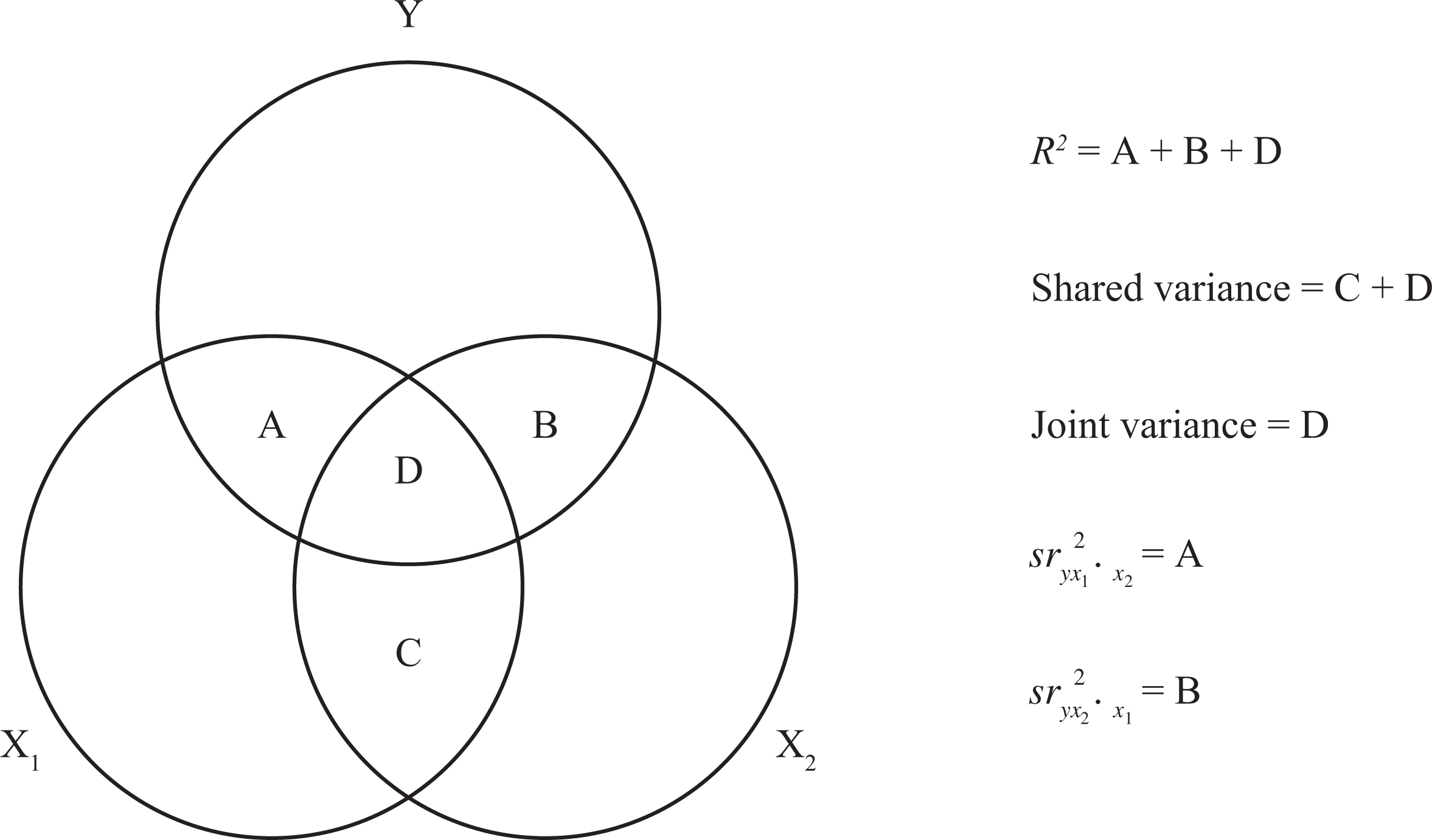
We will define joint variance (JV) as the variance shared by a set of predictors (or independent variables) that is also shared with the criterion (or dependent variable). Venn diagrams, which use circles to represent the variance of constructs, help us to illustrate the joint variance component of two predictors (X₁ and X₂) and a criterion (Y). The joint variance component is depicted in Figure 1 as the combined overlap of the three circles representing the variance of X₁, X₂, and Y, and is labeled “D.” The squared correlation between predictors is the total amount of variance they “share.” The “shared variance” of X₁ and X₂ is the combination of “C” and “D” in Figure 1. The overlap between the circle representing X₁ and the circle representing Y in Figure 1 can also be considered a shared variance as is the overlap between X₂ and Y. In short, joint variance is the shared capability of multiple predictors to explain variance in a criterion.

Figure 1.

Predictors with shared variance.

The issues presented by shared variance, joint variance, or their respective interpretations are not new topics for organizational research scientists, but this does not mean we have a grasp on how to handle them (cf. Darlington, 1968). For example, shared variance is often treated in discussions of common method variance. Common method variance is seen as a problem that must be dealt with either through research methodology or statistical correction. But not all shared variance is a statistical or methodological problem (i.e., the overlap researchers generally hope to find between X₁ or X₂, and Y) and examples selected for reanalysis here were chosen specifically because common method variance is an unlikely alternative explanation. Shared variance may also exist because constructs are redundant (i.e., they are conceptually and empirically indistinguishable).

Predictor constructs may be substantially related to one another for interesting and substantive reasons. We are suggesting the following methods be used when researchers wish to explore the relationships between their variables further, especially when their predictors are correlated and alternative explanations such as construct redundancy and common method variance are considered unlikely. Many systems may exist, a few that we explore here, that could account for the collinearity of predictor variables in a model (we refer to this collinearity or even multicollinearity as joint variance, as the number of variables and magnitude of the correlation between these variables all relate to our definition of joint variance). The following example helps illustrate the point of how constructs may be related to one another and the criterion in a substantive way.

The joint contribution of the predictors in L. R. James's (1998) analysis can be explained by the interplay between AM and critical intellectual skills throughout an individual’s lifetime. Intellectual ability and motivation are clearly important as separate predictors of performance and are conceptually distinguishable as well. We suggest, however, that intellectual ability and motivation also affect one another and jointly determine performance, and this joint effect is interesting and important to better understand.

Consider that most individuals enjoy being successful. It is possible to imagine a young individual attempting a complex task for the first time. We will assume the individual is successful in his or her attempt at working with the complex task. Task success often fills individuals with pride and a sense of accomplishment. This sense of pride and accomplishment leads individuals to believe certain things about their own contribution to success. For example, individuals are more likely to believe that increases in effort lead to even greater performance (Dweck & Leggett, 1988) and that skills can be learned and are not fixed (Dweck, 1986). Eventually, these kinds of beliefs develop into justification mechanisms for behavior (cf. L. R. James, 1998; L. R. James & Mazerolle, 2002) in that individuals justify their actions to themselves and others in terms of these beliefs. Working long hours is framed as necessary for success. Challenging and difficult tasks are perceived as enjoyable and even necessary for self-fulfillment. As individuals pursue ever increasingly difficult tasks, they also gain critical intellectual skills relevant to task achievement. Thus, an individual who attempts difficult tasks and pursues those tasks to successful completion is likely to gain knowledge and skills that will aid in future tasks.

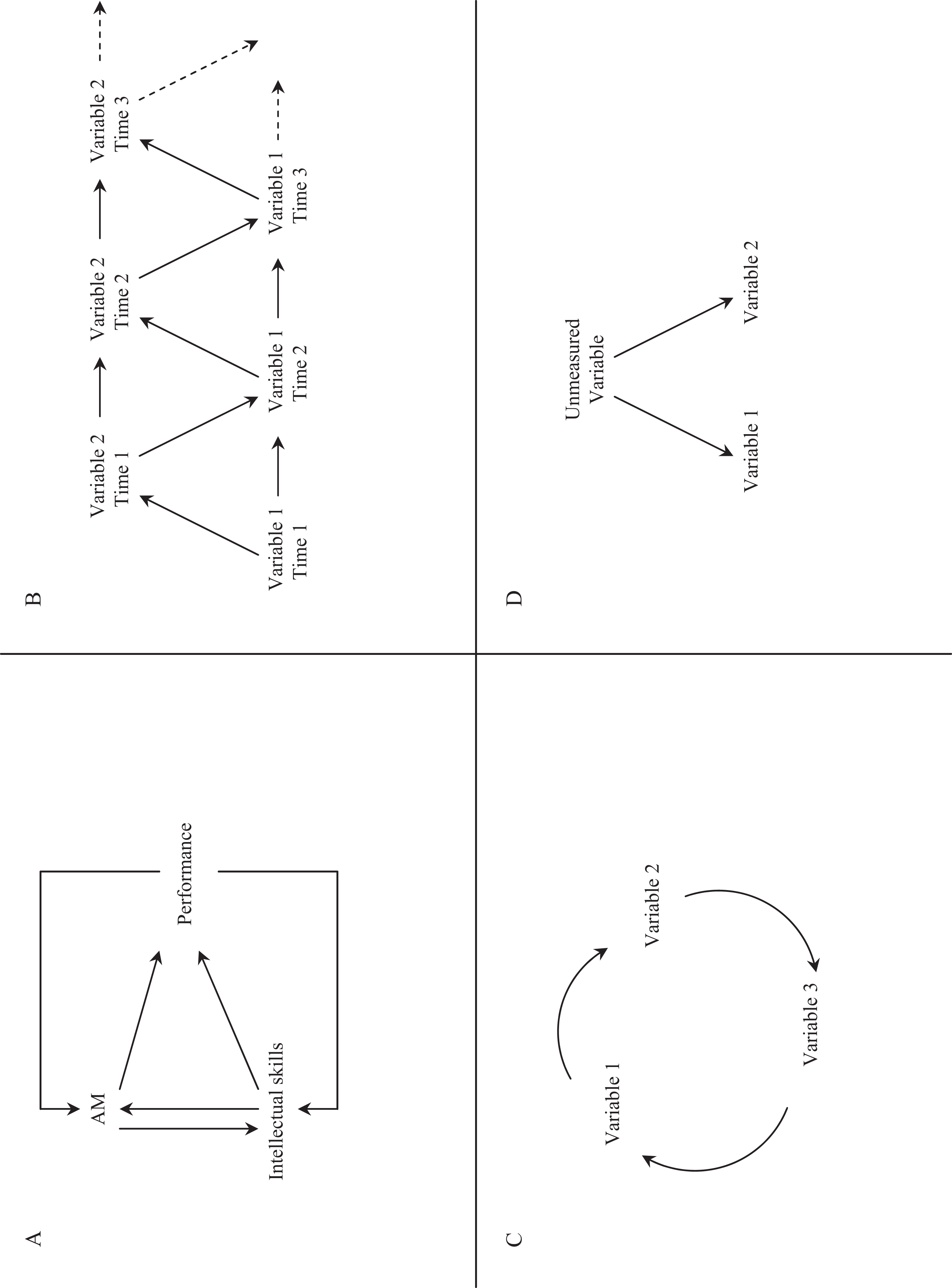
The set of relationships just described is part of a self-reinforcing developmental system. In this example, individuals who put forth effort toward goal accomplishment and who experience success gain certain beliefs about the effectiveness of that effort, which then promotes pursuit of even more difficult goals. The skills learned and knowledge gained during challenging goal pursuit serve as the building blocks and foundations for pursuing more challenging tasks, thus gaining even more skills and knowledge. Moreover, success at each difficult and challenging task leads to feelings of pride and accomplishment. These feelings are not only rewarding but also encourage individuals to want to experience those feelings again. So, they pursue more difficult and challenging tasks (L. R. James & Mazerolle, 2002). This cycle is shown graphically in Figure 2A.

A key product of this continuing cycle is that those who are motivated to achieve also develop the critical skills necessary for achievement. In the case of college students who are voluntarily pursuing a college degree, like the sample used by L. R. James (1998), it is not surprising to see those who are highly achievement motivated also have above-average critical intellectual skills. Furthermore, because of a history of reciprocal influences, these two constructs are jointly (as well as uniquely) related to the scores earned on tests in this performance-oriented environment. In this example, the two predictors are mutually reinforcing but they never converge to the point where they are conceptually indistinguishable (personality and intelligence are separate constructs) and thus construct redundancy is not a likely potential explanation of the joint variance observed here.

A few points are noteworthy in this example. The self-reinforcing developmental cycle that generates the overlap between critical intellectual skills and AM likely begins rather early in the individual’s life. In addition, the correlation between AM and critical intellectual skills, while moderate, is far from perfect. An individual may take up studying and find they are good at it, but another individual may prefer or find first success in athletics or the arts. Individuals simply do not have the time or capability to succeed at and pursue everything they might try. As a result, we would also expect moderate correlations between AM and athletic performance but not necessarily between athletic performance and intelligence (L. R. James & Mazerolle, 2002). Finally, while the theory presented here is supported by data, there are alternative models that could potentially cause the correlation between AM and critical intellectual skills. Our model may not uniquely describe these data, and without longitudinal data collection, we cannot be certain our model is correct.

The Mood Decomposition (MD)

In this section, we overview the MD method described by Mood (1971) for extracting joint variance or “JV.” We limit this introductory effort to models with three independent variables. We use L. R. James's (1998) data set as an example of a three-variable case that has two predictors of interest and one predictor that is not expected to contribute to the explanation of the criterion. Additionally, we provide examples of models that might result in significantly but also substantively correlated predictors that researchers may wish to consider in future theory and research.

MD has been discussed by others and is also referred to as “commonality analysis” or “elements analysis” (cf. Mayeske et al., 1969; Mood, 1969; Newton & Spurrell, 1967a, 1967b; Pedhazur, 1997). We refer to this method here as MD to help delineate our use as a tool for exploring joint variance where elements/commonality analysis is often used as a tool to determine construct redundancy and/or relative importance.

To use MD for two predictors, one starts with the total variance in a criterion accounted for by the predictors. The total variance explained in a model is the sum of the unique variances of each predictor and its relationship with the criterion (i.e., squared semipartial correlations) and the variance that is shared between the predictors that also relates to the criterion (i.e., JV). One can visualize this using Venn diagrams discussed earlier. In Figure 1, the overlap between X₁ and Y represents a squared zero-order correlation (“A” and “D” combined) and the overlap between X₂ and Y is another squared zero-order correlation (“B” and “D” combined). The unique components are also given in Figure 1 (“A” for X₁ and Y, and “B” for X₂ and Y—these are the squared semipartial components). A calculation of total variance explained (R²) gives us an accurate representation of the relationship between the two predictors and the criterion (“A,” “B,” and “D” combined). To interpret the variance explained by regression equations (R²), it is typical for researchers to turn to regression weights (unstandardized B weights or standardized β weights), squared semipartial correlations, and the significance calculations for those weights and/or semipartial correlations.

When using regression, researchers often use total variance explained (R²) as a heuristic to justify continued analyses (i.e., if R² or ▵R² is significant, then testing continues). Researchers rarely interpret variance explained and erroneously rely on regression weights to estimate the size of the effects of their predictors (cf. Courville & Thompson, 2001; Pedhazur, 1997). When researchers interpret only regression weights, semipartials, and the associated significance tests, they are ignoring the joint variance component. In the case of developmental systems where constructs influence one another over time, this could lead to a fallacy when interpreting the outcomes of the regression model. Although individual unique variance components are certainly interesting and important explanatory mechanisms, current data analytic standards unfortunately focus exclusively on these components and disregard the potential of explaining equally interesting and important phenomena that may be uncovered by examining the JV component. In certain instances, such as a self-reinforcing developmental system used to describe L. R. James's (1998) data, we completely miss the joint explanatory component. This is a problem, if the real story of what is happening is described by the continual interplay and reverse causation of the predictors over time leading to a large JV component. By not describing, estimating, and explaining JV, we may be missing an integral part of what we are trying to investigate, which is how various predictors account for variance in our outcomes. In some such systems, the JV may even be the most important aspect of the research.

To extract the JV component is actually rather straightforward with two independent variables. One simply needs to obtain an estimate of overall variance explained (e.g., R²) as well as the squared semipartials for each predictor in the equation. The joint variance is then equal to the difference between the total variance explained and the sum of the squared semipartials (Mood, 1971). This is given below:

Mood Decomposition : JV = R_{y . x_{1} x_{2}}^{2} - (s r_{y x_{1}}^{2} + s r_{y x_{2}}^{2})

and can also be written as:

Mood Decomposition: JV = r_{y x_{1}}^{2} + r_{y x_{2}}^{2} - R_{y . x_{1} x_{2}}^{2}

s r^{2} = R^{2} - R^{2}

If there are three independent variables, there is still a unique contribution of each variable, and this is still indicated by the squared semipartial correlations:

s r_{x_{1}}^{2} = R_{y . x_{1} x_{2} x_{3}}^{2} - R_{y . x_{2} x_{3}}^{2}

s r_{x_{2}}^{2} = R_{y . x_{1} x_{2} x_{3}}^{2} - R_{y . x_{1} x_{3}}^{2}

s r_{x_{3}}^{2} = R_{y . x_{1} x_{2} x_{3}}^{2} - R_{y . x_{1} x_{2}}^{2} .

However, with three independent variables, the joint variance itself can be separated into four distinct components: the joint variance between X₁ and X₂ in explaining Y, the joint variance between X₁ and X₃ in explaining Y, the joint variance between X₂ and X₃ in explaining Y, and the joint variance between X₁, X₂, and X₃ in explaining Y (in terms of Venn diagrams, this can be visualized by four intersecting spheres).

Calculation of the joint variance components in a model with three independent variables is outlined as follows (cf. Mood, 1971). With three independent variables, the variance accounted for by any two variables is a function of the variance accounted for in various models that include the third variable. Calculation of the joint variance of all three predictors is a function of all possible models. Specifically:

{MD}_{x_{1} x_{2}} = R_{y . x_{2} x_{3}}^{2} + R_{y . x_{1} x_{3}}^{2} - R_{y . x_{1} x_{2} x_{3}}^{2} - r_{y . x_{3}}^{2}

{MD}_{x_{1} x_{3}} = R_{y . x_{2} x_{3}}^{2} + R_{y . x_{1} x_{2}}^{2} - R_{y . x_{1} x_{2} x_{3}}^{2} - r_{y . x_{2}}^{2}

{MD}_{x_{2} x_{3}} = R_{y . x_{1} x_{3}}^{2} + R_{y . x_{1} x_{2}}^{2} - R_{y . x_{1} x_{2} x_{3}}^{2} - r_{y . x_{1}}^{2}

M D_{x_{1} x_{2} x_{3}} = R_{y . x_{1} x_{2} x_{3}}^{2} + r_{y . x_{1}}^{2} + r_{y . x_{2}}^{2} + r_{y . x_{3}}^{2} - R_{y . x_{1} x_{2}}^{2} - R_{y . x_{1} x_{3}}^{2} - R_{y . x_{2} x_{3}}^{2} .

Schemes have also been developed to decompose the total variance explained when there are more than three independent variables and there is at least one computer program available to calculate the joint variance elements (Nimon, Lewis, Kane, & Haynes, 2008). We have also developed a spreadsheet to calculate these components from a correlation table with two, three, and four predictor models. The number of components (total joint and unique) rises at an exponential rate with the addition of predictors (2^k − 1, k = number of predictors).¹ These equations and the theoretical explanations behind the components quickly become very complex (cf. Pedhazur, 1997); therefore, we limit our discussion to only two- and three-variable cases.

We now use MD to reanalyze the data of L. R. James (1998) to explore the potential magnitude of the JV components for critical intellectual skills, AM, and gender in explaining intellectual performance as an example of a three-variable model (zero-order correlations for James are given in Table 1 . The MD of these data are:

Gender and ACT : MD = . 427 + . 365 - . 431 - . 360 = . 001

Gender and ACT : MD = . 427 + . 281 - . 431 - . 270 = .00 7

AM and ACT : MD = . 365 + . 281 - . 431 - .0 20 = . 195^{*}

Gender, AM, and ACT : MD = . 431 + .0 20 + . 270 + . 360 - . 281 - . 365 - . 427 = .00 8 .

(where “*” indicates this variable is significant (p < .05) and the discussion of how to compute significance values for these components follows). Less than 1% of the variance explained in the outcome (performance) is explained by each of the joint variance components that include gender. This is not unexpected since gender was not theoretically relevant or significantly correlated with performance or the other predictors. More than 19% of the variance explained in the outcome (performance) is explained by the JV between AM and critical intellectual skills. One might also express the variance explained as a proportion of the JV of each component to the total variance.

Gender and AM : .00 1 / . 431 = .00 2

Gender and ACT : .00 7 / . 431 = .0 16

AM and ACT : . 195 / . 431 = . 452

Gender, AM, and ACT : .00 8 / 0. 431 = .0 19

In other words, nearly half of the criterion variance is accounted for by the joint variance of AM and critical intellectual skills and their relationship with the criterion. Additionally, gender does not play an important unique or joint role in explaining performance.²

Table 1.

James (1998) Correlations; Correlations of Performance, AM, ACT, and Gender

Variable (n = 336)	1	2	3
1. Mean test score	–
2. AM	.52	–
3. ACT	.60	.49	–
4. Gender (0 = male, 1 = female)	−.14	−.07	−.12

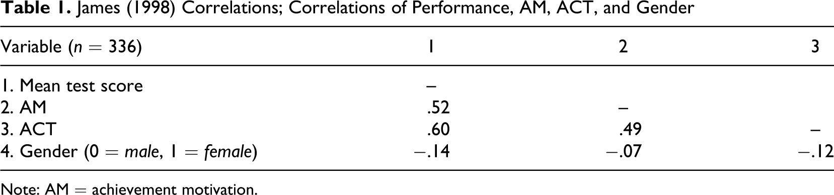
Note: AM = achievement motivation.

L. R. James (1998) was fortunate in that he understood how the variables in his model could potentially work together over time, thus resulting in correlated variables. Based on the notion that intellectual skills have a developmental component (cf. Sternberg & Wagner, 1993; Wagner & Sternberg, 1985, 1986), he suggests, “achievement motivation and skill development are functionally and reciprocally related. One feeds the other, and they are correlated statistically” (L. R. James, 1998, p. 146).

Significance Calculations for Joint Variance Components

One may also calculate the significance values for the joint variance components. Hedges and Olkin (1981), building on the work of Olkin and Siotani (1976) presented the first discussion of significance values for the joint variance component. One cannot use t tests of significance for the joint variance components because they are not independent effects. Instead, significance tests for the joint variance component rely on an asymptotic distribution.

Alf and Graf (1999) and Graf and Alf (1999) greatly simplified the work of Olkin and Siotani (1976) and Hedges and Olkin (1981). The asymptotic variance for each joint variance component is calculated via the delta method given by Olkin and Finn (1995) and is equal to aΦa′ where a is a vector of the partial derivatives of the components comprising the MD equation for the JV component in question and Φ is a variance–covariance matrix of the zero-order correlations and all possible multiple Rs. Calculations for even two predictors is rather complex. The simplified equations for two predictors are given in the appendix.

Models Resulting in Joint Variance Components

There are other models that can also result in the development of substantial joint variance components, though what we present here is not an exhaustive list. The model suggested by L. R. James (1998), given in Figure 2A, is one involving reciprocal causation and self-reinforcement. A simplex model, a model we will explore shortly when we reanalyze other published data, is given in Figure 2B depicting two variables affecting each other over time that can result in large shared variance components. A third possibility, causal loops, is shown in Figure 2C. One can consider causal loops (cf. Hall, 1971; Senge, 1990; Wood & Bandura, 1989) as more complex causal cycles involving more variables than that given in Figure 2A or 2B. Finally, Figure 2D depicts the effects of an unmeasured common cause (James, Mulaik, & Brett, 1982) such as social desirability in self-report data, a higher order causal factor, or other sources of collinearity (i.e., construct redundancy).

There are many types of models researchers may wish to consider when exploring the effects of JV; however, when more than a few variables are included in a model, the interpretation of various JV components may be rather complex (similar in difficulty to developing, interpreting, and reproducing interactions with four or more variables in moderated multiple regression). Researchers may wish to focus on a select few predictors to help aid in interpretation and understanding.³ Many times, the majority of variables in complex models will not be involved in developmental relationships and researchers will need to rely on theory to guide their selection of constructs they subject to more detailed analyses.

Reinterpretation of Prior Studies

Authors have dealt with correlated variables in ways other than Mood’s decomposition method over the years. It is not our intention to criticize the works we explore here but simply to reevaluate them using a different theoretical paradigm and additional statistical techniques. We also demonstrate how structural equation modeling is not exempt from the problems we illustrate with research that used regression as the analytic method.

Heggestad and Kanfer (2005) published data from a laboratory study and reanalyzed data from another study that explored the relationship between self-efficacy, past performance, and current performance. Theoretically, self-efficacy is one’s personal belief in the capability to perform a task. With higher self-efficacy, one is expected to approach a task and regulate behavior differently than if one were to have low self-efficacy. Bandura and his colleagues (cf. Bandura, 1986; Wood & Bandura, 1989) suggest self-efficacy is an important predictor of performance.

To test the effects of past performance and self-efficacy on current performance, Heggestad and Kanfer (2005) used a noun-pair lookup task in a laboratory study and the study they reanalyzed was a managerial simulation. The model they tested, using multiple regression, suggests that self-efficacy is only predictive of performance during early trials of a training program and is not a strong predictor in later trials as suggested by Wood and Bandura (1989). They suggest that the results of Wood and Bandura, which suggest self-efficacy is a significant predictor across successive trials, are likely a result of the method used in analyzing these data. Based on their own findings and the recency principal of Hawkings (1992), Heggestad and Kanfer suggest that self-efficacy is a result of performance instead of a cause of performance.

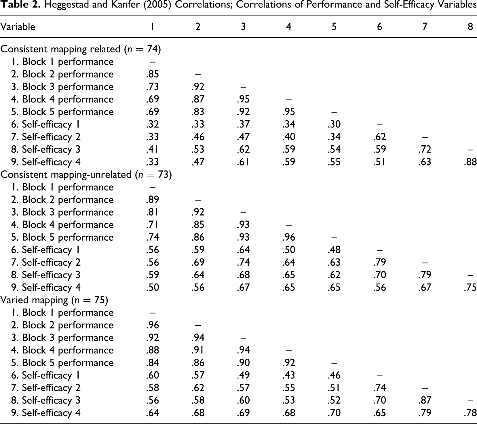
Using the correlation table provided in their article (see our Table 2 ), one can obtain the total variance explained (R²) and the semipartial correlations for self-efficacy and past performance for each phase of the study of Heggestad and Kanfer (2005) for each of their three experiments. Each experiment used a separate sample. The experimental conditions are consistent mapping related, consistent mapping unrelated, and varied mapping and are inconsequential for our discussion and not considered further. With these data, it is possible to calculate the JV components, the proportion of JV to the total variance explained for each performance block analyzed in their study for each experiment, and the significance of the JV components. The JV components provided by an MD, indication of the significance of those components, and proportions of JV to total variance explained are given in Table 3 .

Table 2.

Heggestad and Kanfer (2005) Correlations; Correlations of Performance and Self-Efficacy Variables

Variable	1	2	3	4	5	6	7	8
Consistent mapping related (n = 74)
1. Block 1 performance	–
2. Block 2 performance	.85	–
3. Block 3 performance	.73	.92	–
4. Block 4 performance	.69	.87	.95	–
5. Block 5 performance	.69	.83	.92	.95	–
6. Self-efficacy 1	.32	.33	.37	.34	.30	–
7. Self-efficacy 2	.33	.46	.47	.40	.34	.62	–
8. Self-efficacy 3	.41	.53	.62	.59	.54	.59	.72	–
9. Self-efficacy 4	.33	.47	.61	.59	.55	.51	.63	.88
Consistent mapping-unrelated (n = 73)
1. Block 1 performance	–
2. Block 2 performance	.89	–
3. Block 3 performance	.81	.92	–
4. Block 4 performance	.71	.85	.93	–
5. Block 5 performance	.74	.86	.93	.96	–
6. Self-efficacy 1	.56	.59	.64	.50	.48	–
7. Self-efficacy 2	.56	.69	.74	.64	.63	.79	–
8. Self-efficacy 3	.59	.64	.68	.65	.62	.70	.79	–
9. Self-efficacy 4	.50	.56	.67	.65	.65	.56	.67	.75
Varied mapping (n = 75)
1. Block 1 performance	–
2. Block 2 performance	.96	–
3. Block 3 performance	.92	.94	–
4. Block 4 performance	.88	.91	.94	–
5. Block 5 performance	.84	.86	.90	.92	–
6. Self-efficacy 1	.60	.57	.49	.43	.46	–
7. Self-efficacy 2	.58	.62	.57	.55	.51	.74	–
8. Self-efficacy 3	.56	.58	.60	.53	.52	.70	.87	–
9. Self-efficacy 4	.64	.68	.69	.68	.70	.65	.79	.78

Table 3.

Heggestad and Kanfer (2005) Mood Decomposition

Variables	R²	Semipartials Square, Summed	MD Estimate of JV, R² − ∑ (Semipartial²)	Proportion: JV/R²
Consistent mapping-related
DV = B2P, IVs = B1P, SE1	.72*	.79² + .06² = .63	.72 − .63 = .09	.09/.72 = .13
DV = B3P, IVs = B2P, SE2	.85*	.79² + .05² = .63	.85 − .63 = .22*	.22/.85 = .26
DV = B4P, IVs = B3P, SE3	.90*	.75² + .01² = .56	.90 − .56 = .34*	.34/.90 = .38
DV = B5P, IVs = B4P, SE4	.90*	.76² + (−.01)² = .58	.90 − .58 = .32*	.32/.90 = .36
Consistent mapping-unrelated
DV = B2P, IVs = B1P, SE1	.80*	.68² + .11² = .47	.80 − .47 = .33*	.33/.80 = .41
DV = B3P, IVs = B2P, SE2	.87*	.57² + .15² = .35	.87 − .35 = .52*	.52/.87 = .60
DV = B4P, IVs = B3P, SE3	.87*	.67² + .02² = .45	.87 − .45 = .42*	.42/.87 = .48
DV = B5P, IVs = B4P, SE4	.92*	.71² + .03² = .51	.92 − .51 = .41*	.41/.92 = .45
Varied mapping
DV = B2P, IVs = B1P, SE1	.92*	.73² + (−.01)² = .53	.92 − .53 = .39*	.39/.92 = .42
DV = B3P, IVs = B2P, SE2	.88*	.75² + (−.02)² = .56	.88 − .56 = .32*	.32/.88 = .36
DV = B4P, IVs = B3P, SE3	.89*	.78² + (−.04)² = .61	.89 − .61 = .28*	.28/.89 = .31
DV = B5P, IVs = B4P, SE4	.86*	.61² + .10² = .38	.86 − .38 = .48*	.48/.86 = .56

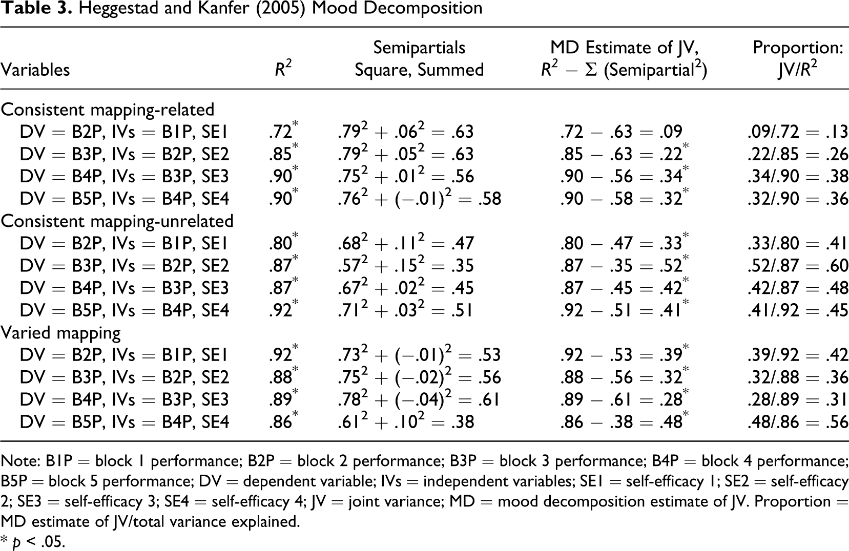
Note: B1P = block 1 performance; B2P = block 2 performance; B3P = block 3 performance; B4P = block 4 performance; B5P = block 5 performance; DV = dependent variable; IVs = independent variables; SE1 = self-efficacy 1; SE2 = self-efficacy 2; SE3 = self-efficacy 3; SE4 = self-efficacy 4; JV = joint variance; MD = mood decomposition estimate of JV. Proportion = MD estimate of JV/total variance explained.

* p < .05.

Heggestad and Kanfer (2005) used multiple regression to estimate the extent to which self-efficacy and prior performance explained the occurrence of current performance. Based on their data that we also analyzed in a stepwise manner with multiple regression to obtain effect sizes and semipartial correlations, we see that the JV component of self-efficacy and previous performance in predicting current performance generally increases over the successive trials. During the early performance stages, the smallest JV component is .09, or 13% of the total variance explained (see Table 3) and is not significant. That is to say, self-efficacy and past performance contribute uniquely and only uniquely in predicting current performance during the early stages of engagement with the task. Through successive trials, the JV component generally increases, and the largest JV component of self-efficacy and prior performance predicting current performance is .52, or 60% of the total variance explained. Simply stated, the effect of the joint component of self-efficacy and past performance is greater than the combined effects of the unique components in explaining current performance during the later stages of task engagement.

Theoretically, the growth in the joint component supports Bandura’s (1986) social cognitive model where past performance informs self-efficacy. Based on Bandura’s predictions, prior performance informs one’s beliefs—self-efficacy—about their expected performance on a future similar task. That is to say, self-efficacy is informed substantially by one’s past experience and having higher self-efficacy then helps individuals in the regulatory process of task pursuit. These regulatory processes include setting higher personal goals and having higher performance expectations (Mitchell, Hopper, Daniels, George-Falvy, & James, 1994; Wood & Bandura, 1989). Our reanalysis of these longitudinal data collected in a controlled environment (i.e., the laboratory), which also matches theory, suggests our interpretation is supported; however, without measures of other constructs such as personal goals and expectations, it is difficult to rule out alternative models.

Although Heggestad and Kanfer (2005) used regression, their proposed model is a simplex model, which is a longitudinal structural model that can be tested with SEM. Therefore, we applied a simplex model to these data using SEM. The models for the three different experimental conditions are given in Figures 3–5. These models include standardized path coefficients for all paths suggested by the simplex model, though many of these paths were not tested by Heggestad and Kanfer in their original regression analysis.

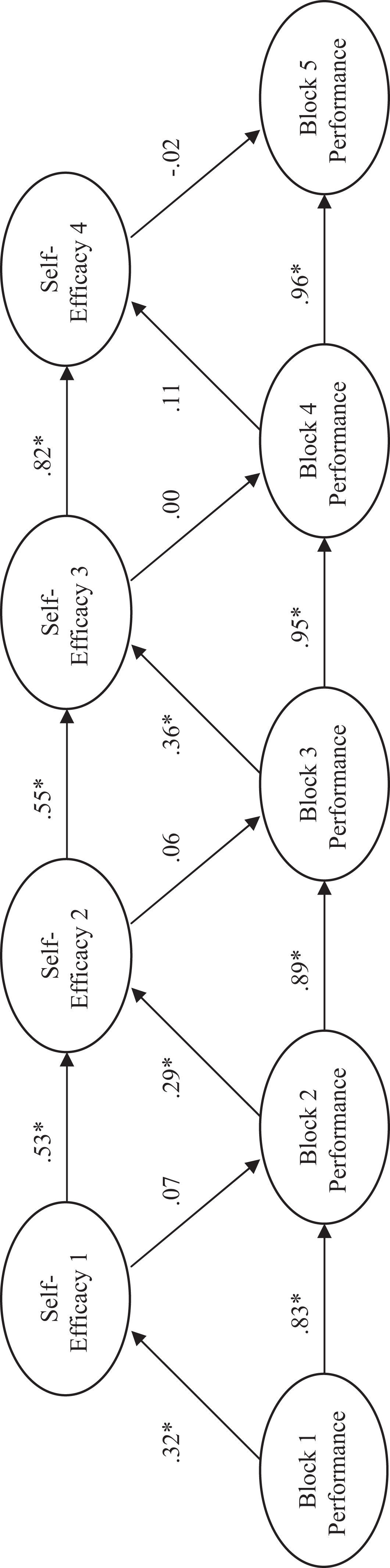
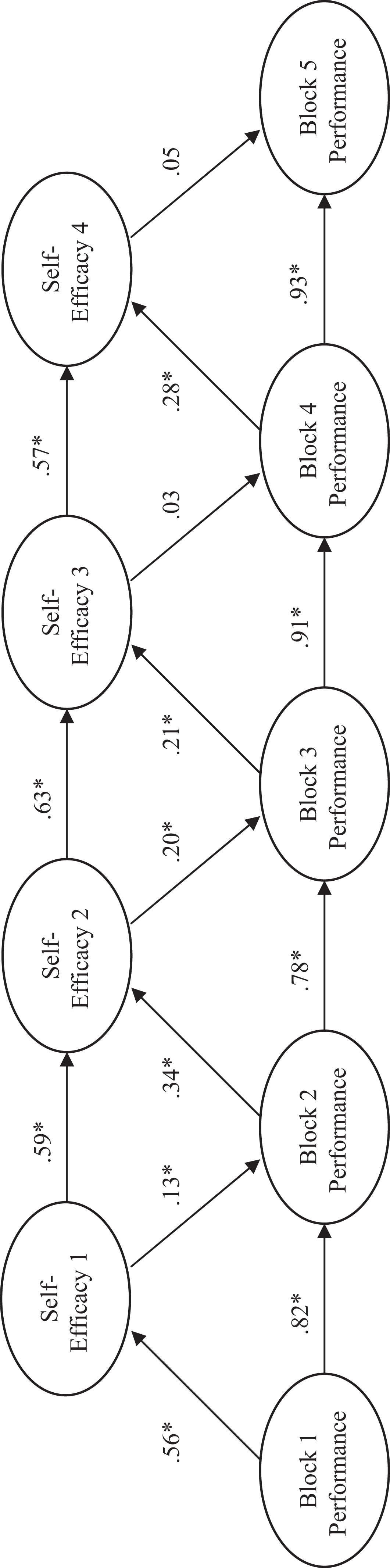
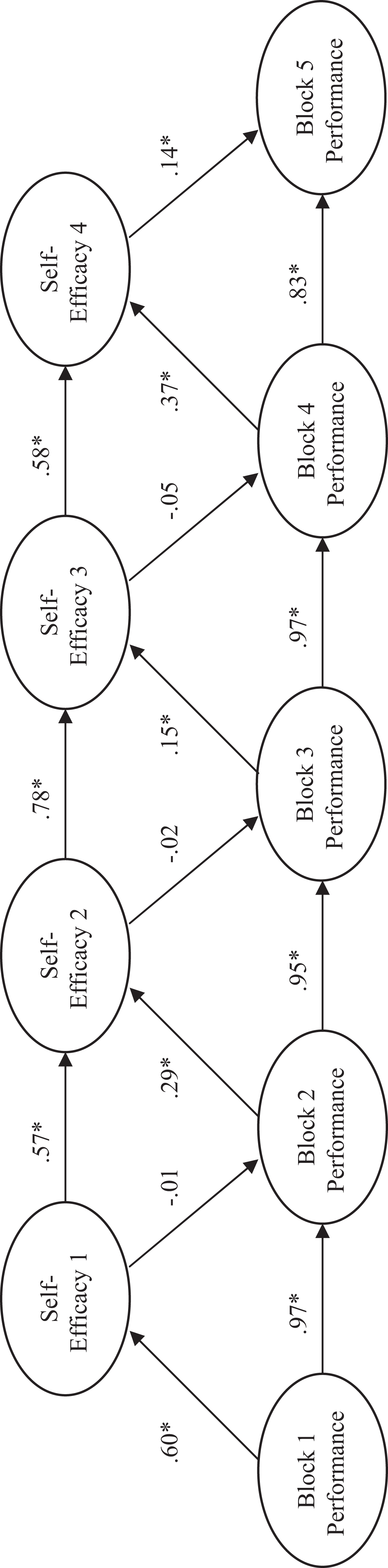
The simplex models given in Figures 3–5 along with the regression models provided by Heggestad and Kanfer (2005) appear to provide evidence in support of their position that self-efficacy is only a result of performance and not a cause since the path coefficients, like the regression weights in the analysis of Heggestad and Kanfer, suggest that self-efficacy is not a significant predictor of performance. The path coefficients are generally significant for paths from performance to self-efficacy, whereas paths from self-efficacy to performance are not. If one is only concerned with the unique effect of various predictors, then past performance is the best predictor of current performance (Heggestad & Kanfer, 2005; Mitchell et al., 1994). If, however, one is concerned with fully describing human growth and development, the exclusive focus on the unique predictive capability of self-efficacy and past performance misses the target. In addition, in this case, without understanding the development of the large joint variance component, one could run the risk of mistakenly suggesting that self-efficacy is not an important predictor of performance. In fact, theory and other data (Mitchell et al., 1994; Wood & Bandura, 1989) suggest that self-efficacy is important because of its role in the self-regulation process.

We would also like to point out that the path coefficients in the structural models and the magnitude of the semipartials in the regression models given in Table 3 do not differ substantially. In short, structural models suffer from the same problem found in regression models. Both the significance tests of regression weights and path coefficients and the interpretation of only these significance tests result in an exclusive focus on the unique predictive capability provided by the variables in the model.

It is commonly accepted practice to not interpret null effects or to consider them as unimportant (cf. Cohen, Cohen, West, & Aiken, 2003; Pedhazur, 1997). When variables are correlated, then interpretation of null findings can be difficult. In this example, Heggestad and Kanfer (2005) elected to interpret the null effect of self-efficacy on current performance in later trials as an indication that self-efficacy was not a useful predictor of current performance. With the tools they used and the data at hand, this is a risky conclusion because the predictors are correlated and it relies on the interpretation of a null finding. In this case, the potential value of self-efficacy cannot be assessed via its unique predictive capability but by its joint relationship with past performance. Even though these data were collected in a longitudinal manner and reanalyzed with a more sophisticated structural model suggested by some to help overcome issues found in regression (Baltes, Parker, Young, Huff, & Atlman, 2004), one might still relegate self-efficacy to a lesser predictive status than what it deserves. With the theoretical perspective and methodological techniques, we provide these authors may have come to a different conclusion.

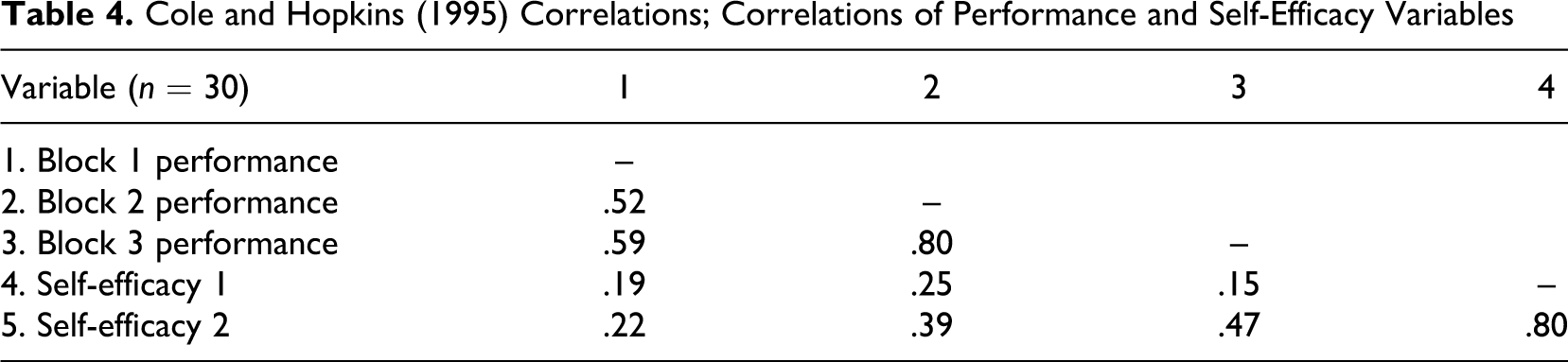
Heggestad and Kanfer (2005) also report data from another study (Cole & Hopkins, 1995) to help support their interpretation that self-efficacy is only a result of performance. The correlations for this study and the MD are given in Tables 4 and 5 , respectively. Once again, the MD results suggest that the JV component between self-efficacy and prior performance increases through the successive trials. Initially, the MD of initial performance and self-efficacy explaining current performance results in a JV component of .04, which is 13% of the explained variance and is not significant. The analysis of the third trial provides a JV component of .19, which is 29% of the explained variance and is significant (p < .05).

Table 4.

Cole and Hopkins (1995) Correlations; Correlations of Performance and Self-Efficacy Variables

Variable (n = 30)	1	2	3	4
1. Block 1 performance	–
2. Block 2 performance	.52	–
3. Block 3 performance	.59	.80	–
4. Self-efficacy 1	.19	.25	.15	–
5. Self-efficacy 2	.22	.39	.47	.80

Table 5.

Cole and Hopkins (1995) Mood Decomposition

Variables	R ²	Semipartials Square, Summed	MD Estimate of JV, R² − ∑ (Semipartial²)	Proportion: JV/R²
DV = B2P, IVs = B1P, SE1	.29*	.482 + .15² = .25	.29 − .25 = .04	.04/.29 = .13
DV = B3P, IVs = B2P, SE2	.67*	.672 + .17² = .48	.67 − .48 = .19*	.19/.67 = .29

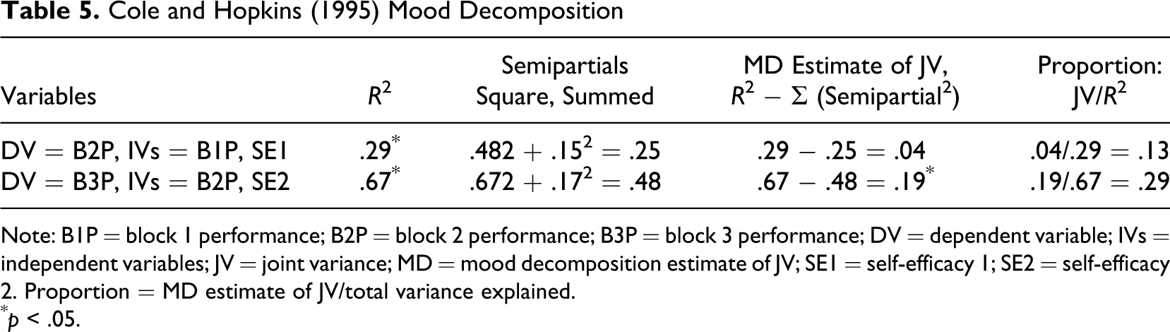
Note: B1P = block 1 performance; B2P = block 2 performance; B3P = block 3 performance; DV = dependent variable; IVs = independent variables; JV = joint variance; MD = mood decomposition estimate of JV; SE1 = self-efficacy 1; SE2 = self-efficacy 2. Proportion = MD estimate of JV/total variance explained.

^*p < .05.

A simplex model was also applied to these data. Similar results as given for Heggestad and Kanfer (2005) were found. Figure 6 shows the model for these data.

Figure 6.

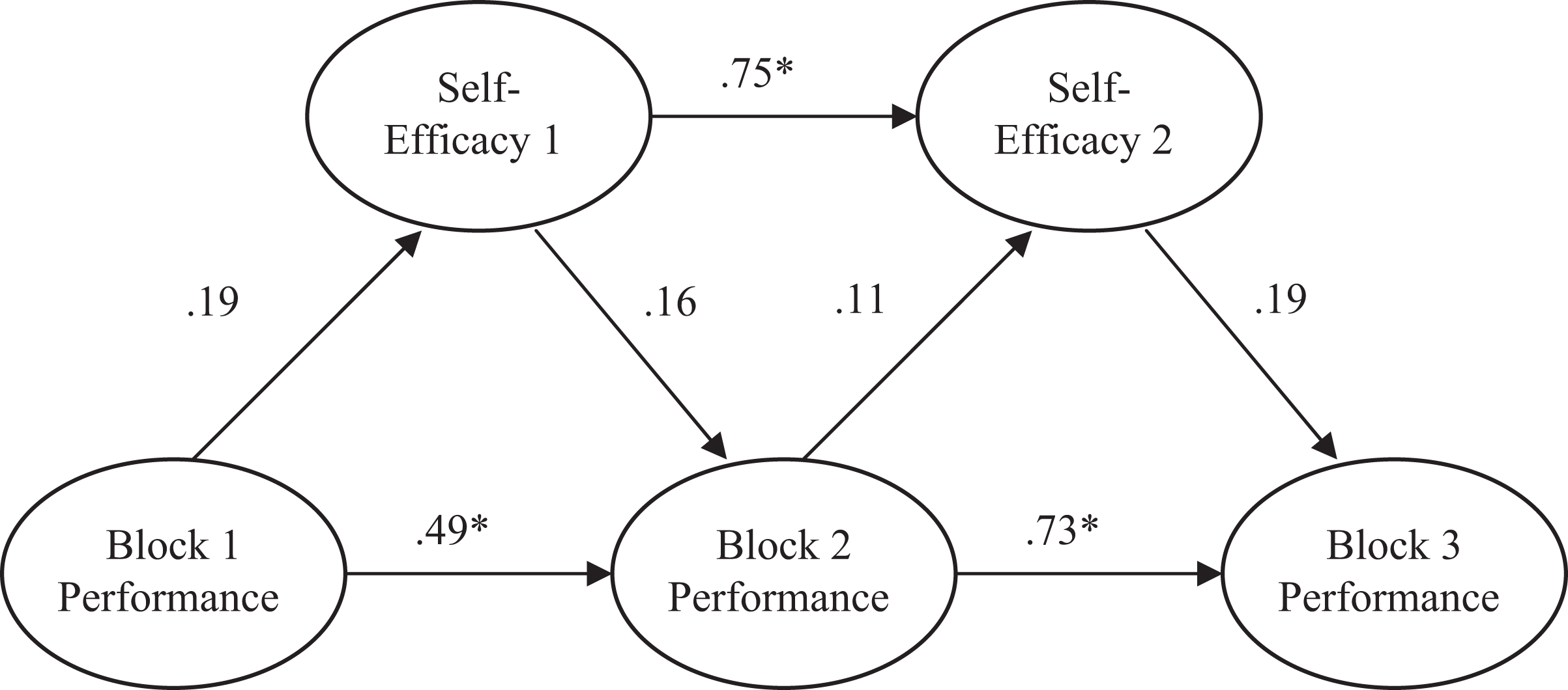
Cole and Hopkins (1995). *p < .05.

Heggestad and Kanfer (2005) appear to be partially correct in suggesting self-efficacy is a result of performance. However, by relying on estimates of unique effects, they may be missing the rest of the story. The relationship between self-efficacy and performance appears to be involved in a developmental cycle. As theory suggests (Bandura, 1986), initial performance on the task helps to inform the individual of the correctness of their self-efficacy belief. This adjusted self-efficacy belief then prompts the individual to regulate their performance on the subsequent experimental trials. The cycle then repeats itself so that the individual’s performance on the trials aids the individual in refining his or her self-efficacy belief even further (Mitchell et al., 1994; Wood & Bandura, 1989). By exploring only regression weights, as is typically done, Cole and Hopkins (1995) and Heggestad and Kanfer miss the growing JV component that explains an increasingly large portion of the variance in the criterion.

Discussion

We have presented a method developed by Mood (1971) for calculating the joint variance components of multiple predictors on a criterion. Additionally, we calculated significance values for these components using an asymptotic distribution. The estimating procedures for the MD have the potential for frequent use. Most studies published today in the organizational sciences discuss a series of constructs and their unique relationships with the criteria of interest. Little or no consideration is given to how two or more predictors may be interrelated through mechanisms such as developmental sequences and reciprocal causation. Instead, researchers often consider moderated relationships as the sum total of possible joint relationships. This creates a significant gap in our research, methodology, and understanding. There are other potential characterizations of JV and shared variance that need to be discussed. In short, there could be a number of reasons that variables are correlated with one another such as common method variance and construct redundancy that do not necessarily represent the substantive effects we are hoping researchers will now consider in more detail in the future. We also discuss our method as a complement to relative importance and finally consider the utility of MD as an explanatory tool.

Common Method Variance

Common method variance and its potential ability to bias study findings is a significant issue in the organizational sciences. Common method variance is the “variance that is attributable to the measurement method rather than to the constructs the measures represent” (Podsakoff, MacKenzie, Lee, & Podsakoff, 2003, p. 879) and may occur when the criteria and predictors are collected from the same source, all at the same time, and using similar measurement techniques. This common method variance could be a major source of JV uncovered by MD (see Figure 2D) as it represents correlations between predictors caused by the research method and not by substantive relationships between the variables under consideration. Same source data are likely to inflate the MD estimates of JV components. This could potentially lead to large JV components when there is truly a much lower joint relationship between the predictor constructs in explaining the criterion. Interpreting JV under these conditions may be problematic.

Construct Redundancy

Another form of collinearity is construct redundancy. The original purpose of this type of correlation partitioning was to determine what predictors were performing well and what predictors were performing poorly in a prediction model and this effect was considered solely as construct redundancy. MD may still represent construct redundancy or variables under consideration that are not measuring separate constructs but instead are measuring the same thing. In a purely predictive sense, there is little reason to care about why constructs are redundant. Tools such as MD become valuable when researchers start to try to develop answers for “why?” questions and we provide an example below that could have been framed in terms of construct redundancy.

Our example is a study by L. A. James and James (1989), who explored how individuals attribute meaning to various environmental factors at work. L. A. James and James proposed, based on the theory of Lazarus (1982, 1984) that individuals appraise their work environment using one higher order factor, “this g-factor comprises a higher order schema for appraising the degree to which the environment is personally beneficial versus personally detrimental (damaging or painful) to the self and therefore to one’s well-being” (L. A. James & James, 1989, p. 740). In short, individuals make an overall good/bad judgment of their work environment that influences how they perceive and report various facets of that work environment.

Researchers are unlikely to argue that a workplace facet considered by L. A. James and James (1989) such as leader trust is conceptually the same as (or redundant to) another workplace facet such as job autonomy also considered by these authors. Yet, the analysis by L. A. James and James using a second-order confirmatory factor analysis (similar to our Figure 2D) suggests these constructs may be highly related. For prediction purposes, measures of leadership trust may function only slightly differently in a prediction equation than job autonomy. Yet, theoretically and practically, the relationships between the facets of the workplace were more interesting than construct redundancy, and we believe the perspective and methods provided here may spur researchers to more deeply consider the reasons for the collinearity among their predictors.

Relative Importance

Researchers in the organizational sciences have long understood that the variance shared between predictors is enigmatic (cf. Darlington, 1968; Johnson & LeBreton, 2004). When researchers test theories, they often hope to demonstrate that one predictor variable is more important to prediction than another variable. It can be difficult to determine with regression coefficients which predictor variable is more important when two (or more) predictors are correlated. To overcome this problem, methodologists have developed multiple ways of exploring the relative importance of the predictor variables compared to one another, one of which is the decomposition developed by Mood (1971). Two of the more advanced techniques at this time are dominance analysis (Azen & Budescu, 2003) and relative weights (Johnson, 2000, 2001; Johnson & LeBreton, 2004).

These methods allow researchers to determine the relative importance of their unique predictors in explaining a criterion variable by essentially partitioning the JV among the predictors. Determining relative importance is a useful analysis tool, but it does not help answer the question we are asking. After using one of these techniques, researchers still have no idea of the magnitude of the variance shared between the predictor variables and how this shared variance helps explain the criterion. Furthermore, these techniques do not allow the researcher to determine whether the JV component itself is a statistically significant and substantive issue that needs consideration. In short, relative importance techniques are focused on simple main effect models that may miss the more complex interrelationships that researchers may be trying to understand. Thus, MD represents a tool complementary to relative importance that can help researchers to understand the complexities of human functioning as well, and we urge researchers to use the tool or tools most theoretically appropriate for their research questions.

Prediction Versus Explanation

We are proposing the use of MD as an additional tool that researchers can use to aid in the explanation of human behavior. Pedhazur (1997), who covers this topic as well, suggests MD cannot be used with data from correlational studies as a tool for generating hypotheses about why variables are related to one another and to a criterion. This position has been well heeded, and researchers have not used MD in this way. We disagree with this position. Contrary to Pedhazur’s (1997) view of correlational research as a blind predictive tool devoid of substantive input, we believe researchers can use correlations and the analysis of such data to test theories and further explanation. Focusing only on the mechanics of the predictive function of correlational data, which Pedhazur adamantly recommends, leaves researchers wanting for more detailed inferences relating to substantive relationships among their constructs.

As an example of our suggested use for MD, Pedhazur (1997) discusses a case where researchers (e.g., Mayeske et al., 1972) found a large JV component between student racial-ethnic group and teacher racial-ethnic group in describing achievement. According to Pedhazur, “It is obvious, however, that the high correlation between student and teacher racial composition does not reflect a lack of specificity of these variables but is primarily a consequence of a policy of segregation” (1997, p. 270). Even though Pedhazur suggests that researchers not do as he has done and develop hypotheses based on results from correlational data sets, we believe his examination of JV using MD to develop a theory about why two variables are correlated (i.e., race of students and teachers), and through this correlation affect achievement, is likely correct. Thus, MD is a tool researchers can use to further theory development, although this development will generally take the form of hypothesis generation rather than the confirmation/disconfirmation of causal inferences.

We believe theoretical consideration is of utmost importance when working with estimates of JV via MD. With cross-sectional data, it is impossible to determine causality. Most researchers are aware of this issue, yet structural analyses with cross-sectional data persist mostly because of a heavy reliance on existing theory. With cross-sectional data in hand, either via a pretest, a first study in a series of studies, or with the reanalysis of published data, researchers can use MD to generate theories and hypotheses. These new hypotheses should then be tested using methods designed to capture the detail and data necessary of confirmatory analyses.

Conclusion

A nearly exclusive reliance on interpretation of regression weights and semipartial correlations in terms of uniquenesses has likely stunted the organizational sciences in terms of both theoretical development and theory testing. We do not believe that estimates of unique components lack importance. Unfortunately, the reliance on these components by our field has provided an overly simplistic view of human and organizational behavior. Our discussion of MD allows researchers to estimate the effect of multiple predictors on a criterion in a way that can shed light on how these predictors are working jointly and the size of this joint influence.

We believe MD is a tool that allows researchers to explore broader aspects of their theories but, in and of itself, is not the solution for the root problem presented here. First, scholars in the organizational sciences must become more methodologically sophisticated. This means being able to both set up complex laboratory and field experiments but also having the mathematical wherewithal to analyze complex data. Simple main effects models will always be important to the organizational sciences, but the complex human development and functioning we are trying to describe is not ruled by these simple formulas. In reality, simple main effect descriptions of human behavior are likely the exception, not the rule (cf. Nettle, 2006).

Footnotes

Notes

Acknowledgment

The authors thank Robert J. Vandenberg, Charles E. Lance, and three anonymous reviewers for comments on earlier versions of this article.

The author(s) declared no conflicts of interest with respect to the authorship and/or publication of this article.

The author(s) received no financial support for the research and/or authorship of this article.

Appendix

References

Alf

E. F.

Graf

R. G.

(1999). Asymptotic confidence limits for the difference between two squared multiple correlations: A simplified approach. Psychological Methods, 4, 70–75.

Azen

Budescu

D. V.

(2003). The dominance analysis approach for comparing predictors in multiple regression. Psychological Methods, 8, 129–148.

Baltes

B. B.

Parker

C. P.

Young

L. M.

Huff

J. W.

Atlman

(2004). The practical utility of importance measures in assessing the relative importance of work-related perceptions and organizational characteristics on work-related outcomes. Organizational Research Methods, 7, 326–340.

Bandura

(1986). Social foundations of thought and action: A social cognitive theory. Englewood Cliffs, NJ: Prentice Hall.

Budescu

D. V.

(1993). Dominance analysis: A new approach to the problem of relative importance of predictors in multiple regression. Psychological Bulletin, 114, 542–551.

Cohen

West

Aiken

L. S.

(2003). Applied multiple regression/correlation analysis for the behavioral sciences. 3rd ed. Mahwah, NJ: Lawrence Erlbaum.

Cole

B. L.

Hopkins

B. L.

(1995). Manipulations of the relationship between reported self-efficacy and performance. Journal of Organizational Behavior Management, 15, 95–135.

Conger

A. J.

(1974). A revised definition for suppressor variables: A guide to their identification and interpretation. Educational and Psychological Measurement, 34, 35–46.

Courville

Thompson

(2001). Use of structure coefficients in published multiple regression articles: β is not enough. Educational and Psychological Measurement, 61, 229–248.

10.

Darlington

R. B.

(1968). Multiple regression in psychological research and practice. Psychological Bulletin, 69, 161–182.

11.

Dweck

C. S.

(1986). Motivational processes affecting learning. American Psychologist, 41, 1040–1048.

12.

Dweck

C. S.

Leggett

E. L.

(1988). A social-cognitive approach to motivation and personality. Psychological Review, 95, 256–273.

13.

Gordon

R. A.

(1968). Issues in multiple regression. American Journal of Sociology, 73, 592–616.

14.

Graf

R. G.

Alf

E. F.

(1999). Correlations redux: Asymptotic confidence limits of partial and squared multiple correlations. Applied Psychological Measurement, 23, 116–119.

15.

Hall

D. T.

(1971). A theoretical model of career subidentity development in organizational settings. Organizational Behavior and Human Performance, 6, 50–76.

16.

Hawkings

R. M. F.

(1992). Self-efficacy: A predictor but not a cause of behavior. Journal of Behavior Therapy and Experimental Psychiatry, 23, 251–256.

17.

Hedges

L. V.

Olkin

(1981). The asymptotic distribution of commonality components. Psychometrika, 46, 331–336.

18.

Heggestad

E. D.

Kanfer

(2005). The predictive validity of self-efficacy in training performance: Little more than past performance. Journal of Experimental Psychology: Applied, 11, 84–97.

19.

James

L. A.

James

L. R.

(1989). Integrating work environment perceptions: Explorations into the measurement of meaning. Journal of Applied Psychology, 74, 739–751.

20.

James

L. R.

(1998). Measurement of personality via conditional reasoning. Organizational Research Methods, 1, 131–163.

21.

James

L. R.

Mazerolle

M. D.

(2002). Personality in work organizations. Thousand Oaks, CA: Sage.

22.

James

L. R.

Mulaik

S. A.

Brett

J. M.

(1982). Causal analysis: Assumptions, models, and data. Beverly Hills, CA: Sage.

23.

Johnson

J. W.

(2000). A heuristic method for estimating the relative weight of predictor variables in multiple regression. Multivariate Behavioral Research, 35, 1–19.

24.

Johnson

J. W.

(2001). Determining the relative importance of predictors in multiple regression: Practical applications of relative weights. In Columbus

(Ed.), Advances in psychology research: Vol. 5 (pp. 231–251). Huntington, NY: Nova Science.

25.

Johnson

J. W.

LeBreton

J. M.

(2004). History and use of relative importance indices in organizational research. Organizational Research Methods, 7, 238–257.

26.

Lazarus

R. S.

(1982). Thoughts on the relations between emotion and cognition. American Psychologist, 37, 1019–1024.

27.

Lazarus

R. S.

(1984). On the primacy of cognition. American Psychologist, 39, 124–129.

28.

Mayeske

G. W.

Cohen

W. M.

Wisler

C. E.

Okada

Beaton

A. E.

Proshek

J. M.

… Tabler

K. A.

(1969). A study of our nation’s schools. Washington, DC: U.S. Department of Health, Education, and Welfare, Office of Education.

29.

Mayeske

G. W.

Cohen

W. M.

Wisler

C. E.

Okada

Beaton

A. E.

Proshek

J. M.

… Tabler

K. A.

(1972). A study of our nation’s schools. Washington, DC: U.S. Government Printing Office.

30.

Mitchell

T. R.

Hopper

Daniels

George-Falvy

James

L. R.

(1994). Predicting self-efficacy and performance during skill acquisition. Journal of Applied Psychology, 79, 506–517.

31.

Mood

A. M.

(1969). Macro-analysis of the American educational system. Operations Research, 17, 770–784.

32.

Mood

A. M.

(1971). Partitioning variance in multiple regression analyses as a tool for developing learning models. American Educational Research Journal, 8, 191–202.

33.

Nettle

(2006). The evolution of personality variation in humans and other animals. American Psychologist, 61, 622–631.

34.

Newton

R. G.

Spurrell

D. J.

(1967a). A development of multiple regression analysis of routine data. Applied Statistics, 16, 51–64.

35.

Newton

R. G.

Spurrell

D. J.

(1967b). Examples of the use of elements for clarifying regression analyses. Applied Statistics, 16, 165–172.

36.

Nimon

Lewis

Kane

Haynes

R. M.

(2008). An R package to compute commonality coefficients in the multiple regression case: An introduction to the package and practical example. Behavior Research Methods, 40, 457–466.

37.

Olkin

Finn

J. D.

(1995). Correlations redux. Psychological Bulletin, 118, 155–164.

38.

Olkin

Siotani

(1976). Asymptotic distribution of functions of a correlation matrix. In Ikeda

(Ed.), Essays in probability and statistics (pp. 235–251). Tokyo, Japan: Shinko Tsusho.

39.

Pedhazur

E. J.

(1997). Multiple regression in behavioral research: Explanation and prediction. 3rd ed. Belmont, CA: Wadsworth-Thomson Learning.

40.

Podsakoff

P. M.

MacKenzie

S. B.

Lee

Podsakoff

N. P.

(2003). Common method biases in behavioral research: A critical review of the literature and recommended remedies. Journal of Applied Psychology, 88, 879–903.

41.

Senge

P. M.

(1990). The fifth discipline: The art and practices of the learning organization. New York, NY: Doubleday.

42.

Sternberg

R. J.

Wagner

R. K.

(1993). The geocentric view of intelligence and job performance is wrong. Current Directions in Psychological Science, 2, 1–4.

43.

Tzelgov

Henik

(1991). Suppression situations in psychological research: Definitions, implications, and applications. Psychological Bulletin, 109, 524–536.

44.

Velicer

W. F.

(1978). Suppressors variables and the semipartial correlation coefficient. Educational and Psychological Measurement, 38, 953–958.

45.

Wagner

R. K.

Sternberg

R. J.

(1985). Practical intelligence in real-world pursuits: The role of tacit knowledge. Journal of Personality and Social Psychology, 49, 436–458.

46.

Wagner

R. K.

Sternberg

R. J.

(1986). Tacit knowledge and intelligence in the everyday world. In Sternberg

R. J.

Wagner

R. K.

(Eds.), Practical intelligence: Nature and origins of competence in the everyday world (pp. 51–83). New York, NY: Cambridge University Press.

47.

Wood

Bandura

(1989). Social cognitive theory of organizational management. Academy of Management Review, 14, 361–384.