A Critical Examination of Common Beliefs About Partial Least Squares Path Modeling

Abstract

Partial least squares path modeling (PLS) was developed in the 1960s and 1970s as a method for predictive modeling. In the succeeding years, applied disciplines, including organizational and management research, have developed beliefs about the capabilities of PLS and its suitability for different applications. On close examination, some of these beliefs prove to be unfounded and to bear little correspondence to the actual capabilities of PLS. In this article, we critically examine several of these commonly held beliefs. We describe their origins, and, using simple examples, we demonstrate that many of these beliefs are not true. We conclude that the method is widely misunderstood, and our results cast strong doubts on its effectiveness for building and testing theory in organizational research.

Keywords

partial least squares statistical and methodological myths and urban legends structural equation modeling

Partial least squares path modeling (PLS) was developed in the 1960s and 1970s by Herman Wold (cf. Jöreskog & Wold, 1982) as an alternative to LISREL. However, Dijkstra (1983) soon proved that if PLS is used as an estimator for structural equation models (SEMs), the parameter estimates are both inconsistent and biased, leading to abandonment of further development. Nevertheless, PLS experienced a renaissance in more applied disciplines with proponents such as Fornell and Bookstein (1982) and later Chin (1998) and Hulland (1999), and recent publications in management journals indicate that its use is increasing (Antonakis, Bendahan, Jacquart, & Lalive, 2010; Echambadi, Campbell, & Agarwal, 2006; Gruber, Heinemann, Brettel, & Hungeling, 2010; Hair, Sarstedt, Pieper, & Ringle, 2012; Peng & Lai, 2012; Reinartz, Haenlein, & Henseler, 2009; Sosik, Kahai, & Piovoso, 2009). Following Atinc, Simmering, and Kroll (2011) we reviewed four leading management journals, Academy of Management Journal, Journal of Applied Psychology, Journal of Management, and Strategic Management Journal, and found 27 studies that used PLS, which are listed in Table 1; a third of these studies were published in the past 5 years, supporting the argument that the use of PLS is becoming more common.

Table 1.

Use of PLS in Selected Management Journals Ordered by Year (Academy of Management Journal, Journal of Applied Psychology, Journal of Management, Strategic Management Journal).

Article	Summary of Description of the Method and Why It Was Used	How PLS Was Used		Relationship to SEM			Capabilities of PLS
Article	Summary of Description of the Method and Why It Was Used	Validation of Measurement	Null Hypothesis Significance Testing	PLS Is SEM	Simultaneous Eqs./Path Analysis	PLS Is Latent Variable Analysis	Distribution Free/Nonnormal Data	Models or Reduces Measurement Error	Works Well With Small Samples	Appropriate for Early/Exploratory Research
Cool, Dierickx, and Jemison, 1989	PLS is an SEM method that can be used when the data are not appropriate for LISREL and that avoids many of the problems of LISREL.	×	×	×	×	×	×	×	×
Duxbury and Higgins, 1991	PLS is an extremely powerful multivariate analysis technique for testing structural models of latent variables. PLS is ideal for early stages of theory testing because of unrestrictive assumptions.	×	×			×	×			×
Howell and Avolio, 1993	Description of the method is copied from Duxbury and Higgins (1991).	×	×	×	×	×	×	×		×
Johansson and Yip, 1994	PLS is a causal modeling technique that has less stringent assumptions about the data than LISREL.	×	×	×			×
Meznar and Nigh, 1995	PLS is a “second-generation” method that examines the relationships in the theoretical model simultaneously. PLS was used because it is well suited for assessing predictive relationships.	×	×	×	×	×				×
Birkinshaw, Morrison, and Hulland, 1995	PLS is a powerful multivariate analysis technique that belongs to the same family of techniques as LISREL. PLS was used because estimating the model as separate equations would lead to biased estimates.	×	×	×	×		×		×
Sosik, Avolio, and Kahai, 1997	PLS is an SEM method that does not make assumptions about distributions, observation independence, or variable metrics and, because of this, is preferable over LISREL.	×	×	×			×
Olk and Young, 1997	PLS is an SEM method that permits formative indicators.	×	×	×	×	×
Birkinshaw, Hood, and Jonsson, 1998	PLS is one of the so-called second-generation techniques that allow simultaneous modeling of relationships.	×	×	×	×		×			×
Shamir et al., 1998	PLS is a powerful multivariate technique that is ideal for testing structural models with latent variables.	×	×	×		×	×		×
Delios and Beamish, 1999	No description of the method given. PLS was used because the objective of the study was prediction of the dependent variable.	×	×		×		×		×
Howell and Hall-Merenda, 1999	PLS is a structural equation modeling technique that has less stringent assumptions about the data. PLS was used because it is appropriate for early stages of theory development.	×	×	×			×			×
Avolio, Howell, and Sosik, 1999	Identical with Howell and Hall-Merenda (1999).	×	×	×			×			×
Shea and Howell, 2000	PLS is a structural equation modeling technique used to analyze theoretically derived models linking constructs and their measures. PLS was used because it is appropriate for early stages of theory development.		×	×			×		×	×
Sarkar, Echambadi, and Harrison, 2001	No description of the method or why it was used was provided.	×	×			×	×	×
Tsang, 2002	No description of the method or why it was used was provided.	×	×	×
Robins, Tallman, and Fladmoe-Lindquist, 2002	PLS is a latent variable technique that can model both reflective and formative indicators and is well suited to assessing predictive relations.	×	×			×	×
Bass, Avolio, Jung, and Berson, 2003	PLS is a structural equation modeling technique that has less stringent assumptions about the data.	×	×	×			×		×
Cording, Christmann, and King, 2008	PLS is a powerful multivariate analysis technique of the same family as LISREL. PLS was used because it allows multiple indicators, does not require a large sample, and does not assume multivariate normality.	×	×	×	×	×	×	×	×
Zott and Amit, 2008	No description of the method or why it was used was provided.	×
Tiwana, 2008	PLS is an SEM method. It was used because of small sample size.	×		×					×
Groth, Hennig-Thurau, and Walsh, 2009	PLS is a distribution-free structural equation modeling technique with less constraints and statistical specifications than LISREL.	×	×	×			×
Ashill and Jobber, 2010	PLS is an SEM-based methodology. PLS was chosen because of the small sample size and exploratory nature of the research.	×	×	×					×	×
Gruber et al., 2010	PLS is a variance-based structural equation modeling technique. It was used for its ability to accommodate formative indicators.	×	×	×
Crossland and Hambrick, 2011	PLS is a form of structural equation modeling that is particularly useful for small samples and in early stages of theory development.	×	×	×		×			×	×
Cheung, Myers, and Mentzer, 2011	PLS is an SEM method. PLS was used because the primary concern of the study is with the prediction of a dependent endogenous variable		×	×		×
Wang and Bansal, 2012	No description of the method except that it permits variables to have both antecedents and consequences in the model.	×	×
Number of surveyed studies		25	25	21	8	11	17	4	10	9
Percentage of surveyed studies		93	93	78	30	41	63	15	37	33

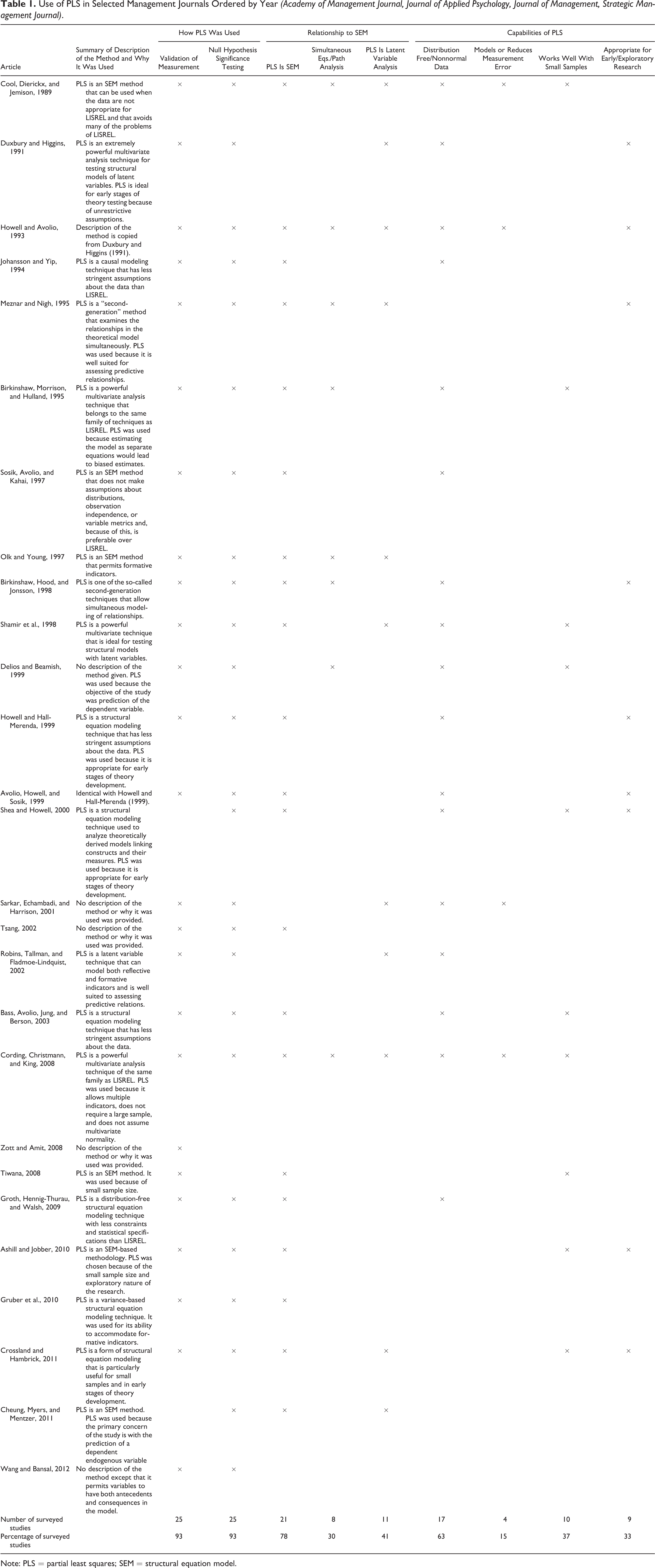
Note: PLS = partial least squares; SEM = structural equation model.

In contrast to its popularity in management research, PLS has been largely ignored in research methods journals. For example, there are no articles in Organizational Research Methods addressing the PLS method. In our review of other top research methods journals, we found one article about PLS (Henseler & Chin, 2010) published in Structural Equation Modeling and one article (Dijkstra, 1983) in Journal of Econometrics. No articles about PLS were found in Psychological Methods, Psychological Bulletin, or Econometrica.

The absence of articles on PLS in the research methods literature has led researchers in disciplines such as strategic management (Hulland, 1999), operations management (Peng & Lai, 2012), marketing (Hair, Ringle, & Sarstedt, 2011), group research (Sosik et al., 2009), and information systems (Gefen, Rigdon, & Straub, 2011) to develop their own guidelines on how to perform and evaluate PLS-based studies. We argue that most of these articles present an overly positive picture of the method, with some aggressively promoting the method as a “silver bullet” (Hair et al., 2011), a “success story” (Vinzi, Chin, Henseler, & Wang, 2010), or as a method with “genuine advantages” (Henseler & Sarstedt, 2013). However, many of these articles are not based on statistical theory or simulation studies but are based on beliefs about the method that earlier, similar articles have presented, leading to the perpetuation of commonly held beliefs that have not been demonstrated, that is, methodological myths and urban legends (Vandenberg, 2006).

This article addresses some of these beliefs and shows that they are incorrect or correct only with strong qualifications. Given the growing popularity of PLS-based studies in management research, this is a timely and important topic.

Overview of the PLS Method

As originally presented, the statistical model of PLS is identical to the original LISREL model (Jöreskog & Wold, 1982). This model is given in Equations 1 and 2, where $η$ designates latent variables, $y$ designates the indicator variables, $π$ and $β$ represent regression coefficients, and $ν$ and $ε$ represent random errors.¹

η_{j} = β_{j 0} + \sum_{i} β_{j i} η_{i} + ν_{j}

Equation 1, called the inner model

y_{k_{j}} = π_{k_{j}}_{0} + π_{k_{j}} η_{j} + ε_{k_{j}}

Equation 2, called the outer model

The model is estimated by replacing the latent variables $η$ with composites $Y$ that are weighted sums of their indicators (Equation 3) and then estimating all path coefficients ( $β$ ) and factor loadings ( $π$ ) by running a separate ordinary least squares regression for each endogenous variable in the model.

Y_{j} = \sum_{k_{j}} ω_{k_{j}} y_{k_{j}}

(Equation 3, latent variable estimates)

At this level of abstraction, PLS estimation is identical to estimation with OLS regression on summed scales or factor scores. PLS differs from these methods in that the indicator weights $ω$ are based on the estimated model and the sample data. The iterative weighting process begins by approximating the latent variables as unweighted sums and then iteratively adjusting the indicator weights and approximate latent variable scores $\tilde{Y}$ in two steps, called inner and outer estimation, until the weights and scores converge (Table 2).

During the inner estimation step, new latent variable score approximations are calculated as weighted sums of “adjacent” latent variable score approximations, that is, of latent variables related to the focal variable by regression relationships. During the outer estimation step, new indicator weights $\tilde{ω}$ are calculated in either of two ways. In Mode A estimation, the manifest variables $y$ are regressed on the approximations $\tilde{Y}$ :

y_{k_{j}} = {\tilde{ω}}_{k_{j} 0} + {\tilde{ω}}_{k_{j}} {\tilde{Y}}_{j} + {\tilde{ε}}_{k_{j}} .

Equation 4, Mode A estimation

In Mode B estimation,² the approximations $\tilde{Y}$ are regressed on the manifest variables $y$ :

{\tilde{Y}}_{j} = \sum_{k_{j}} {\tilde{ω}}_{k_{j}} y_{k j} + {\tilde{d}}_{j} .

Equation 5, Mode B estimation

The new indicator weights are then used to estimate new latent variable score approximations for the following iteration of inner estimation. The basic PLS algorithm is shown in Table 2. The only difference between PLS and OLS is the different method of indicator weighting.

Table 2.

The Basic PLS Algorithm (Lohmöller, 1989, p. 29).

Stage 1	Iterative estimation of weights and LV scores; starting at Step 4 with arbitrary weights, repeat Steps 1 to 4 until convergence is achieved
	Inner weights (centroid weighting scheme)^a $v_{j i} = \{\begin{matrix} s i g n c o v (Y_{j}, Y_{i}) & i f Y_{j} a n d Y_{i} a r e a d j a c e n t \\ 0 & o t h e r w i s e \end{matrix}$
	Inside approximation ${\tilde{Y}}_{j} = \sum_{i} v_{j i} Y_{i}$
	Outer weights; estimate $ω_{k j}$ in Equation 4 (Mode A) or Equation 5 (Mode B) using ordinary least squares regression
	Outside approximation $\tilde{Y_{j}} = f_{j} \sum_{k_{j}} {\tilde{ω}}_{k_{j}} y_{k_{j}}$
Stage 2	Estimation of path and loading coefficients by ordinary least squares regression from Equation 1 (path coefficients) and Equation 2 (loadings coefficients) where the latent variables $η_{j}$ are replaced by their estimates $Y_{j}$
Stage 3	Estimation of the means of latent and manifest variables as weighted sums

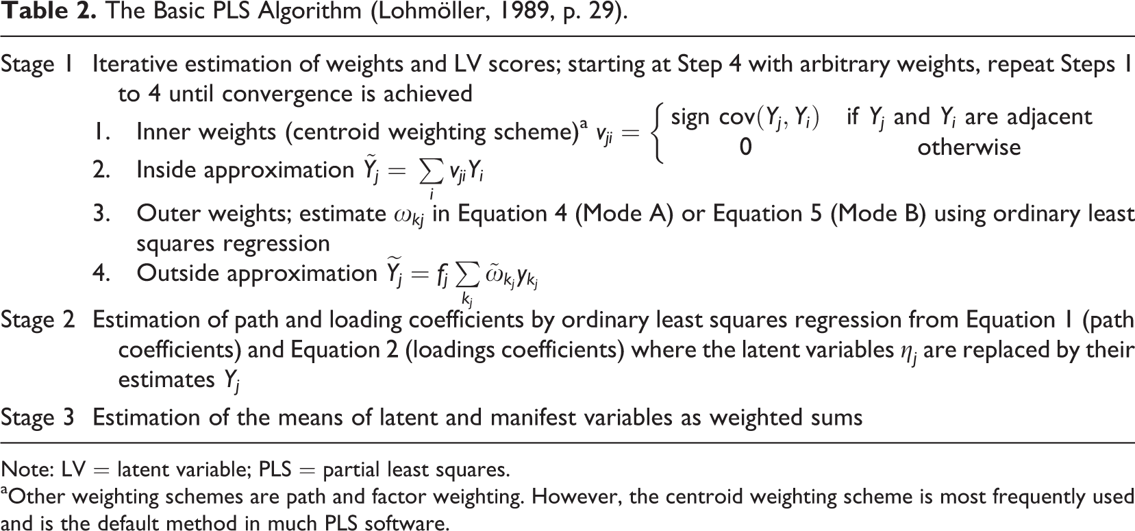
Note: LV = latent variable; PLS = partial least squares.

^aOther weighting schemes are path and factor weighting. However, the centroid weighting scheme is most frequently used and is the default method in much PLS software.

Statistical Myths and Urban Legends About the PLS method

We now discuss six beliefs about PLS that emerged from our review of the articles in Table 1 and the numerous articles providing guidelines on how to use the method and assess the results. Each subsection starts by describing the myth and reviewing its origins and supporting evidence. We use the simple two-construct model shown in Figure 1, along with simulated data sets, to demonstrate that many features ascribed to the PLS algorithm do not hold even in a simple example. The simple example was chosen for the sake of illustration and the ability to derive results analytically. However, we emphasize that our following arguments make no assumptions about the form or complexity of the model.

Figure 1.

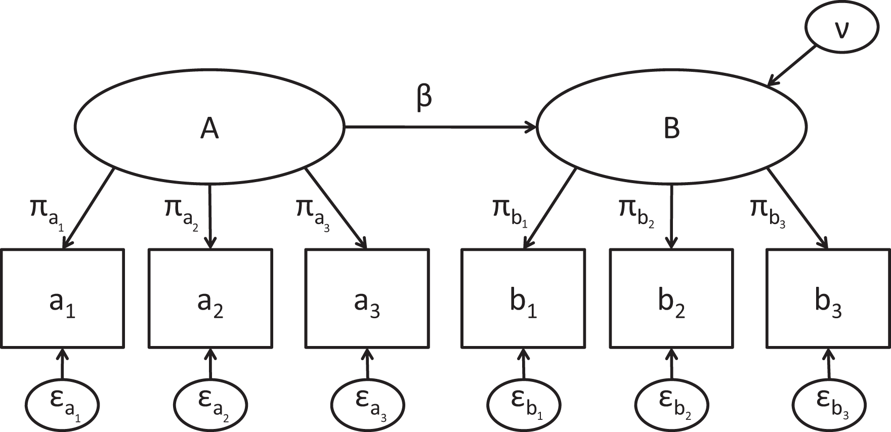
Example model with two constructs.

Myth 1: PLS Has Advantages Over Traditional Methods Because It Is an SEM Estimator

Almost every article in Table 1 and all of the guidelines on PLS present it as an SEM method, with some even emphasizing its differences from OLS on summed scales or factor scores (e.g., Gefen et al., 2011). This characterization cannot be found in the original articles on PLS (e.g., Wold, 1985b). Rather, it is attributable to a widely cited article by Fornell and Bookstein (1982). Nevertheless, even the original characterization as a latent variable modeling technique is misleading. In contrast to claims by many studies in Table 1, PLS does not estimate path models with latent variables, but with composites, and instead of using path analysis with simultaneous equations, PLS uses separate OLS regressions. Thus, it is conceptually closer to OLS regressions on summed scales or factor scores than to covariance structure analysis.

Although PLS can technically be argued to be an SEM estimator, so can OLS regression with summed scales or factor scores: Both fit the definition of the term estimator (Lehmann & Casella, 1998, p. 4) because they provide some estimates of model parameters. This, however, does not mean that PLS or OLS are good estimators in the sense of being consistent and unbiased. An estimator is consistent if its estimates converge to the population value as the sample size increases. It is unbiased if the mean of repeated estimates using samples drawn from the same population approaches the population value as the number of samples increases. PLS has been shown to have neither of these properties. In fact, Wold (e.g., 1985b) is quite clear that PLS estimates are inconsistent, Dijkstra (1983) presented a proof of this, and more recent PLS literature (e.g., Chin, 1998) also readily acknowledges that PLS estimates are biased.

In addition to providing inconsistent and biased estimates, the lack of an overidentification test is another disadvantage of PLS over SEM. Paths between variables in a simultaneous equations model can be constrained to zero. Such constraints make the model overidentified and allow testing whether the constrained model fits the data. Thus, this overidentification test can be used to rule out endogeneity (unmodeled dependencies) that would otherwise cause inconsistency of estimates (Antonakis et al., 2010). Overidentification tests also allow the researcher to rule out alternative causes, which is a key step in testing a model causally (Antonakis et al., 2010; Bollen, 1989, chap. 3). Because no overidentification test is available for PLS, PLS cannot test a model causally, but is limited to estimating statistical associations.

Despite the evidence, many of the reviewed articles argue that PLS supports causal modeling (Birkinshaw, Hood, & Jonsson, 1998; Cool, Dierickx, & Jemison, 1989; Delios & Beamish, 1999; Johansson & Yip, 1994; Shea & Howell, 2000), and some researchers have the misconception that using PLS avoids inconsistent and biased parameter estimates. For example, Birkinshaw, Morrison, and Hulland (1995) write that “to avoid obtaining biased and inconsistent parameter estimates for these equations, the [hypothesized model] must be analyzed using a multivariate estimation technique such as two-stage least squares or PLS” (p. 647). However, of these two estimators, only two-stage least squares is consistent.

In summary, although the argument that PLS is an SEM estimator is technically true, it is as correct to state that OLS regression is an SEM estimator. The lack of unbiasedness and consistency means that both methods will provide erroneous estimates. This, and the lack of an overidentification test, means that any potential advantage that might be obtained by specifying a research problem as an SEM model is lost (Antonakis et al., 2010; McDonald, 1996). The claim that PLS provides advantages because it is an SEM method is a methodological myth, and the current practice of labeling PLS as an SEM method, although correct in a strict technical sense, is very misleading.

Myth 2: PLS Reduces the Effect of Measurement Error

Some of the articles in Table 1 and some of the reviewed guidelines argue that PLS reduces the effects of measurement errors. Although most of these articles fail to explain how this is accomplished, any such advantage over OLS must be a result of the indicator weighting in PLS, because this is the only difference between PLS and OLS. As with most other myths that we discuss, this myth also seems to originate from the work by Fornell and Bookstein (1982), who state, without providing justification, that PLS separates irrelevant variance from the model. This unproven notion has been replaced more recently by the idea that PLS increases the reliability of the composites by using indicator weighting to minimize error (e.g., Gefen et al., 2011).

We first illustrate the effect of measurement error for Mode A weighting. Consider indicator 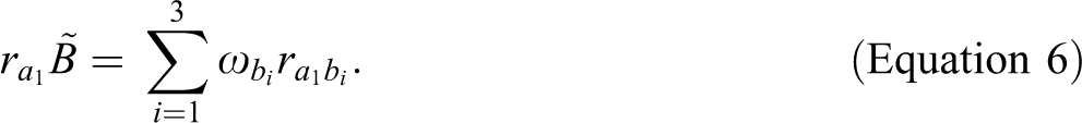$a_{1}$ in the example shown in Figure 1. Starting with Steps 1 and 2 in Stage 1 (Table 2), the inner weighting and inside approximation yield an $\tilde{A}$ that is approximated by $\tilde{B}$ , which is a composite of $b_{1}$ , $b_{2}$ , and $b_{3}$ . In Step 3 of Stage 1 (Table 2), $a_{1}$ is weighted based on its correlation with this composite. This correlation is simply a weighted sum of the correlations between $a_{1}$ and the indicators $b_{1}$ , $b_{2}$ , and $b_{3}$ . It can be written as a function of the current values of the indicator weights ( $ω$ ) and the correlations between the indicators (r), as follows:

r_{a 1 \tilde{B}} = \sum_{i = 1}^{3} ω_{b_{i}} r_{a_{1} b_{i}}

Equation 6

In the two-construct example, under the default PLS assumption of standardized latent variables and indicators, the correlation between two indicators is the sum of the correlation caused by common antecedents and error correlation. Using covariance algebra one can write the correlation between indicators as follows:

r_{a_{i} b_{j}} = π_{a_{i}} β λ π_{b_{j}} + ε_{a_{i} b_{j}} .

Equation 7

Substituting Equation 7 into Equation 6 and rearranging the terms yields

r_{a_{1} \tilde{B}} = π_{a_{1}} β \sum_{i = 1}^{3} ω_{b_{i}} π_{b_{i}} + \sum_{i = 1}^{3} ω_{b_{i}} ε_{a_{1} b_{i}} .

Equation 8

This equation shows that although the indicator weighting system takes the indicator reliability into account, it is highly sensitive to the correlated errors $e_{a_{1} b_{i}}$ in the second sum of Equation 8, contrary to recent claims (Gefen et al., 2011). This is problematic because, as a result of sampling variation, the errors are never exactly uncorrelated, even for correct models. When the latent variables are not correlated ( $β$ = 0), the effect is more pronounced because the first term in Equation 8 vanishes and only the effect of correlated errors remains.

With PLS Mode B, the indicator weights are defined based on regressions of the latent variable estimate on their indicators. Hence, they are also affected by the correlations between indicators of the same construct. In this regression, a set of highly reliable indicators is highly collinear, resulting in suppression effects and instability of the regression coefficients and the resulting indicator weights.

To illustrate these effects numerically for our two-construct example model, we simulated data for two conditions, one with no effect between constructs ( $β = 0$ ) and one with a moderate size effect ( $β = 0.3$ ). We set the factor loadings to 0.6, 0.7, and 0.8. Similar loadings have been used in prior studies (Goodhue, Lewis, & Thompson, 2012; Reinartz et al., 2009). We used 100 observations as the sample size, which is fairly typical for a PLS study. We performed 500 replications for both experimental conditions. The models were estimated using the plspm package for R (Sanchez & Trinchera, 2012). We generated the indicator data by first generating a sample of construct true scores and then used these to generate the indicator data. This enabled us to calculate the reliability of the construct estimates directly as a squared correlation between the true scores and estimated latent variable values. Figure 2 compares the reliability of PLS Mode A and PLS Mode B. We also included summed scales as it is the simplest way to construct composite variables that any other method should exceed to be considered useful (McDonald, 1996).

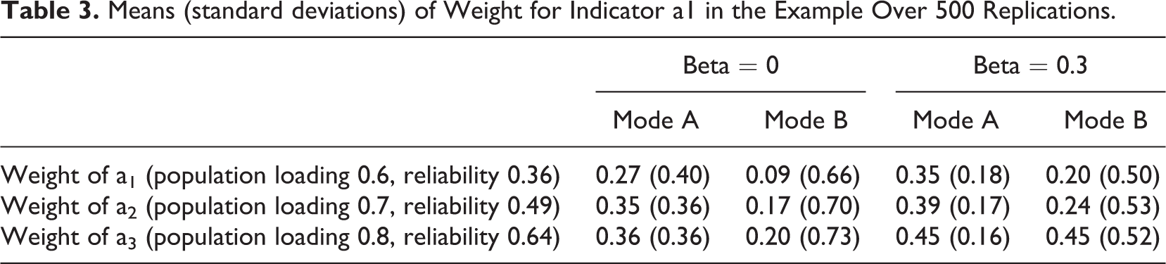
Figure 2 shows that for both PLS modes, summed scales provide better (more reliable) construct scores, and PLS Mode B performs substantially worse than PLS Mode A. The reason for this lower reliability can be seen in Table 3, which shows that, although on average more reliable indicators are weighted more highly, the effect of random correlations causes large variance in the weights, so that any individual replication is very unlikely to have weights even close to an optimal combination. In addition, the collinearity and suppression effects for Mode B estimation are seen clearly in the higher standard deviation of the weights. The lower means of Mode B weights are a result of occasional negative weights caused by collinearity.

Figure 2.

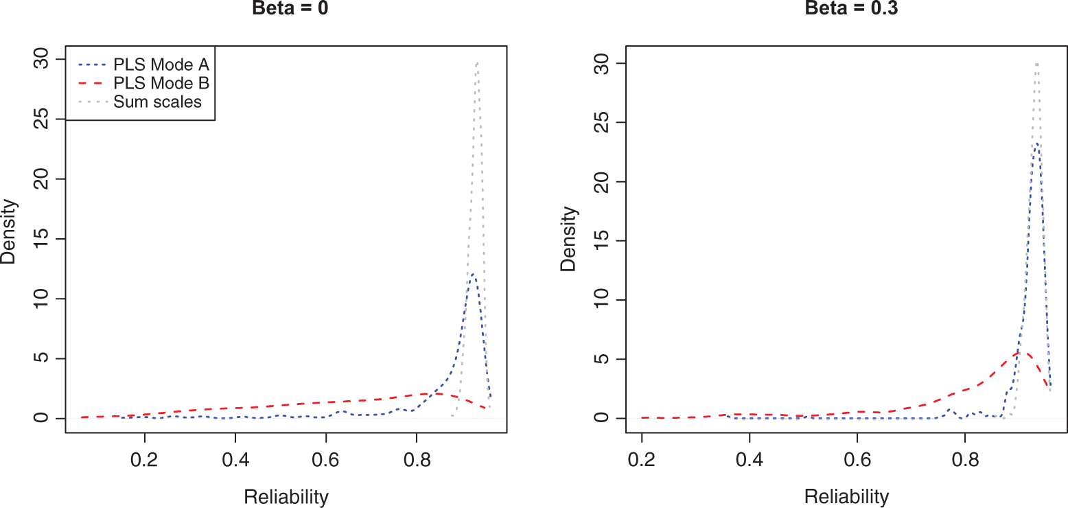
Distribution of reliability for partial least squares (PLS) Mode A, PLS Mode B, and summed scales in the two-construct model over 500 replications.

Table 3.

Means (standard deviations) of Weight for Indicator a1 in the Example Over 500 Replications.

	Beta = 0		Beta = 0.3
	Mode A	Mode B	Mode A	Mode B
Weight of a₁ (population loading 0.6, reliability 0.36)	0.27 (0.40)	0.09 (0.66)	0.35 (0.18)	0.20 (0.50)
Weight of a₂ (population loading 0.7, reliability 0.49)	0.35 (0.36)	0.17 (0.70)	0.39 (0.17)	0.24 (0.53)
Weight of a₃ (population loading 0.8, reliability 0.64)	0.36 (0.36)	0.20 (0.73)	0.45 (0.16)	0.45 (0.52)

We now show how the weighting affects the regression estimates between the latent variables. The standardized path estimate (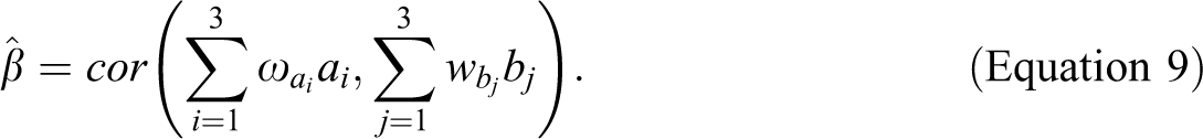 $\hat{β}$ ) between composites $A$ and $B$ is equal to their correlation:

\hat{β} = c o r (\sum_{i = 1}^{3} ω_{a_{i}} a_{i}, \sum_{j = 1}^{3} w_{b_{j}} b_{j}) .

Equation 9

In PLS, the weights are chosen so that the construct estimates are standardized. Thus, the correlation is equal to the covariance, and one can write the covariance of sums as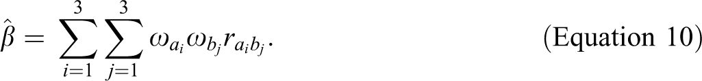

\hat{β} = \sum_{i = 1}^{3} \sum_{j = 1}^{3} ω_{a_{i}} ω_{b_{j}} r_{a_{i} b_{j}} .

Equation 10

Substituting Equation 7 into this and rearranging the terms yields the following:

\hat{β} = β \sum_{i = 1}^{3} \sum_{j = 1}^{3} ω_{a_{i}} ω_{b_{j}} π_{a_{i}} π_{b_{j}} + \sum_{i = 1}^{3} \sum_{j = 1}^{3} ω_{a_{i}} ω_{b_{j}} ε_{a_{i} b_{j}} .

Equation 11

Equation 11 shows that not only the indicator weights but also the path coefficient estimates are affected by the correlated errors. The bias caused by unmodeled correlations is well known (Zimmerman & Williams, 1977), but the joint effect that causes this bias to be amplified by PLS has not been documented in prior literature. 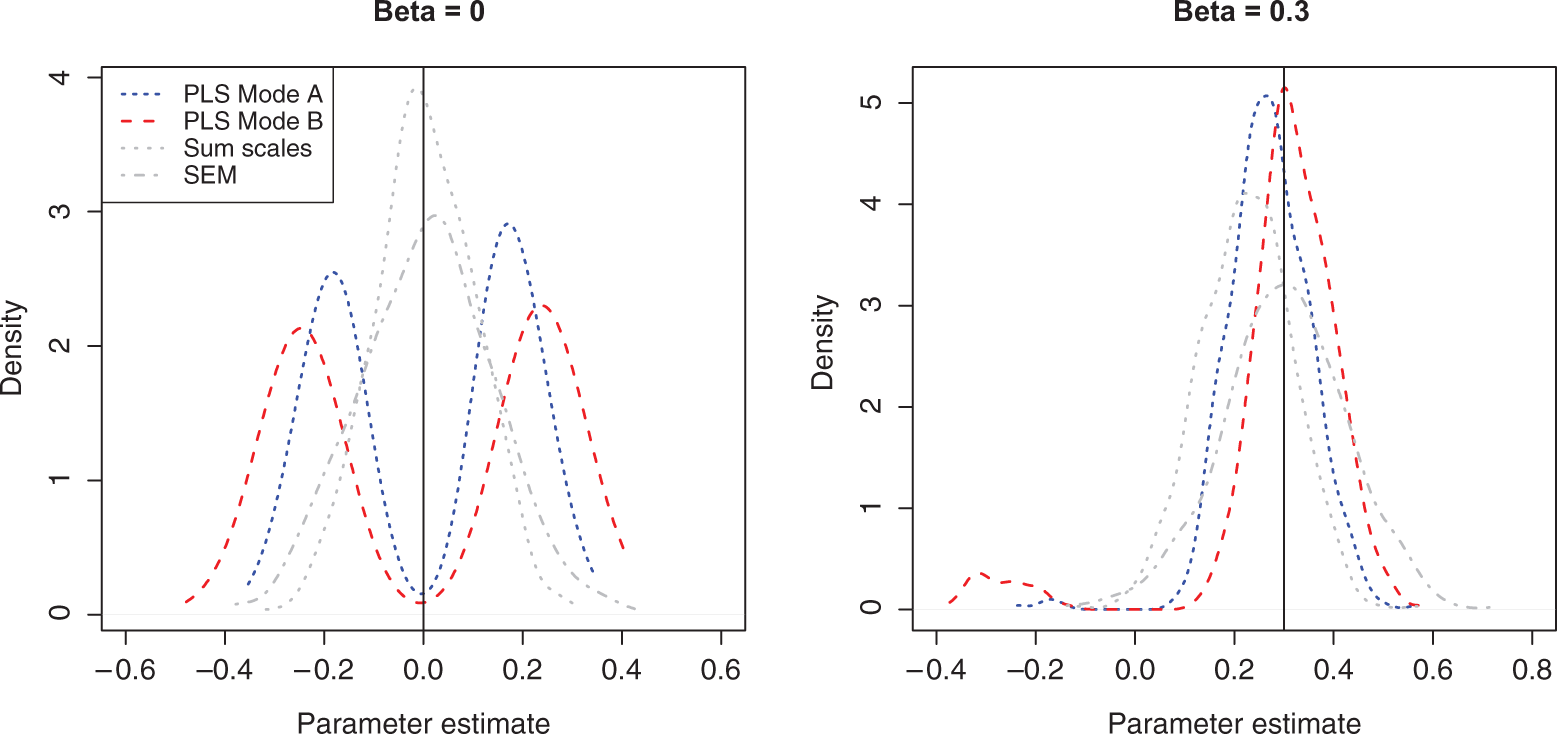This is illustrated in Figure 3, which shows that the parameter estimates obtained from PLS are strongly biased away from zero, whereas no such bias exists when the model is estimated with regression on summed scales or SEM.³ This effect is especially pronounced when $β = 0$ where both Mode A and Mode B estimation produce a bimodal distribution of estimates, symmetrical around 0. These artificially inflated parameter estimates can lead to artificial inflation of statistical significance and incorrect inference.

Figure 3.

Distribution of parameter estimates for partial least squares (PLS) Mode A, PLS Mode B, summed scales, and structural equation modeling (SEM) in the two-construct model, 500 replications.

In contrast to the unsubstantiated claims that PLS reduces the effect of measurement error, we have shown that the indicator weights are strongly affected by error correlations and even the small chance correlations caused by sampling variation are sufficient to affect the weights, resulting in lower reliability composites than even simple summed scales.

The options available for reducing the effect of measurement error with composite variables are limited because any linear composite of indicators that contain error will also be contaminated with error. Random error in the composites causes attenuation of bivariate correlations resulting in bias in the regression estimates. Although it is possible to apply a correction and then use the disattenuated correlations in regression analysis, ML estimation of SEM models has superseded this approach (Cohen, Cohen, West, & Aiken, 2003, pp. 38-39, 473-474).

Myth 3: PLS Can Be Used to Validate Measurement Models

Most of the studies listed in Table 1 use PLS to validate measurement models, and many (e.g., Shamir, Zakay, Breinin, & Popper, 1998; Tiwana, 2008) even assume that PLS can be used to conduct a confirmatory factor analysis. Many researchers seem to also assume that statistics that are typically presented with the PLS results constitute a de facto model test: 7 of the articles listed in Table 1 use the terms model test, testing the model, or similar terminology. Again, these are beliefs that do not originate from Wold, who did not discuss model testing, validation, or fit, but rather used the term test for predictive relevance (without however clearly defining this concept).

The model assessment criteria currently used can be attributed to Fornell and Bookstein (1982), who presented a set of heuristics for assessing PLS models. The most commonly used are the composite reliability (CR) metric and the average variance extracted (AVE) statistic, which are both more or less directly based on factor loading estimates. In addition to these, a family of goodness-of-fit (GoF) indices exists that are calculated on the basis of the endogenous variable R² values and indicator communalities (cf. Henseler & Sarstedt, 2013). There are also various standardized root mean squares of different model residuals (SRMR) that Lohmöller (1989) proposed to be used for model assessment, but we are not aware of any applications of these criteria.

Because the use of GoF indices was recently comprehensively and convincingly debunked by Henseler and Sarstedt (2013) and because of the obscurity of the SRMR indices, we focus on the AVE and CR statistics, which are commonly used in the studies that we reviewed. Aguirre-Urreta, Marakas, and Ellis (in press) showed that the CR indices are severely biased estimate of reliability of the composites. Moreover, the same issues apply also to the AVE statistic. First, their definitions do not include information about the indicator weights (Fornell & Larcker, 1981, pp. 45-46) but assume unweighted composites, which is intentionally violated in a PLS analysis. Second, they are based on factor loadings, but PLS does not calculate factor loadings, but composite loadings (McDonald, 1996, p. 248). These are always higher than factor loadings as they also explain part of the error variance, whereas a factor analysis explains only the common variance between the indicators.⁴ Consequently, the CR and AVE statistics are also overestimated.

To show the effect of model misspecifications on the AVE, CR, (relative) GoF, and (indicator) SRMR statistics and to demonstrate that these heuristics are unable to reliably identify when the model does not fit data, we calculated these model quality metrics for our two-construct model with 500 replications (Table 4). The estimated model is always our two-construct example, and we vary the population model to make the estimated model misspecified (“Misspecified A, B, C” in Table 4). The last column in Table 4 shows the percentage of models in each condition that a researcher would accept as valid, based on commonly used cutoff values for the different heuristics.⁵ This percentage should be high for the true model and low for the misspecified models. However, results show that this number is high for the composite reliability heuristic across all conditions; researchers are likely to accept all misspecified models as valid. This number is low for the SRMR heuristic across all conditions; researchers are likely to also reject the true model as invalid. The situation is even worse for the rGoF heuristic. By this heuristic, researchers are likely to reject only the true model and are likely to accept only the misspecified models. Finally, the two AVE-based heuristics appear to detect only the third misspecified model, making them unreliable indicators of misspecified models.

Table 4.

Model Fit Indices for the Example Model Estimated With Data From Four Different Population Models.

Statistic	5%	Median	95%	Accept (%)
Composite reliability	0.875	0.940	0.960	98.0
Average variance extracted	0.563	0.646	0.695	98.2
AVE–highest squared corr.	0.454	0.563	0.631	100
Relative goodness of fit	0.620	0.859	0.971	28.6
Std. root mean square residual	0.076	0.090	0.112	13.6
Composite reliability	0.711	0.844	0.895	95.4
Average variance extracted	0.426	0.497	0.557	48.0
AVE–highest squared corr.	–0.025	0.075	0.193	89.2
Relative goodness of fit	0.882	0.934	0.971	88.0
Std. root mean square residual	0.148	0.179	0.211	0
Composite reliability	0.917	0.947	0.965	100
Average variance extracted	0.596	0.658	0.710	100
AVE–highest squared corr.	–0.012	0.072	0.165	92.2
Relative goodness of fit	0.955	0.979	0.993	100
Std. root mean square residual	0.080	0.093	0.110	4.2
Composite reliability	0.542	0.783	0.861	82.4
Average variance extracted	0.392	0.452	0.517	11.2
AVE–highest squared corr.	–0.265	–0.175	–0.081	0.2
Relative goodness-of-fit	0.904	0.958	0.991	94.8
Std. root mean square residual	0.184	0.213	0.244	0

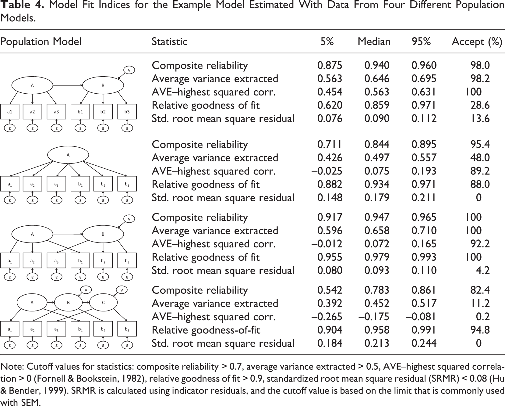
Note: Cutoff values for statistics: composite reliability > 0.7, average variance extracted > 0.5, AVE–highest squared correlation > 0 (Fornell & Bookstein, 1982), relative goodness of fit > 0.9, standardized root mean square residual (SRMR) < 0.08 (Hu & Bentler, 1999). SRMR is calculated using indicator residuals, and the cutoff value is based on the limit that is commonly used with SEM.

In contrast to these heuristics, the χ² test of model fit provides a statistically sound way of identifying misspecified models for medium and large sample sizes,⁶ and the field of psychometrics provides decades of guidance on how to validate measurement with factor analysis (cf. Nunnally, 1978). If desired, factor loadings can be obtained with common factor analysis, and the reliability of a composite with arbitrary weights can be estimated as described by Raykov (1997; see Aguirre-Urreta et al., in press, for how to apply the procedure with PLS analysis). Because of these better alternatives, the measurement model should never be evaluated based on the composite loadings produced by PLS or any statistic derived from these. In summary, we conclude that the idea that PLS results can be used to validate a measurement model is a myth.

Myth 4: PLS Can Be Used for Testing Null Hypotheses About Path Coefficients

Almost all of the articles listed in Table 1 use PLS for null hypothesis significance testing (NHST) of path coefficients, a practice that can be traced back to Fornell and Bookstein (1982). Under NHST, statistical inferences are made based on the p value, which is defined as “the probability of obtaining a value of a test statistic…as large as the one obtained—conditional on the null hypothesis being true” (Nickerson, 2000, p. 247). Thus, NHST relies on a known sampling distribution of the test statistic when the null hypothesis of no effect holds.

The current practice in PLS studies is to use bootstrapping to estimate the standard errors for the parameter estimates, calculate the ratio of a parameter estimate to its standard error, and compare this statistic to the t distribution to obtain the p value. The use of a t distribution assumes a normal distribution of the underlying parameter estimates. However, as shown in Figure 3, the distribution is not normal but of bimodal shape when the null hypothesis of no effect holds ( $β = 0)$ . The exact distribution of the path coefficients is unknown as it depends on the sampling distribution of the indicator weights, which is unknown (Dijkstra, 1983). Thus, because NHST requires a test statistic with a known sampling distribution, the PLS path estimates cannot be used in NHST.

The use of bootstrapped confidence intervals (Wood, 2005) is an alternative to NHST for statistical inference. Even this approach can be problematic with PLS: Bootstrapping relies on the assumption that the bootstrap estimates follow the same distribution as the original statistic, but this is not always the case, leading to incorrect inference (cf. Bollen & Stine, 1992). Figure 4 shows the parameter estimate distribution for 500 replications of the simulation estimates and, for the first 5 of these replications, shows the bootstrap distribution of the parameters. It is clear that the bootstrapped replications do not follow the original sampling distribution in our simple example model.⁷ Thus, we conclude that bootstrapped confidence intervals of PLS estimates should not be used for making statistical inferences until further research is available to show under which conditions, if any, the bootstrapped distribution follows the sampling distribution of the PLS parameter estimate.

Figure 4.

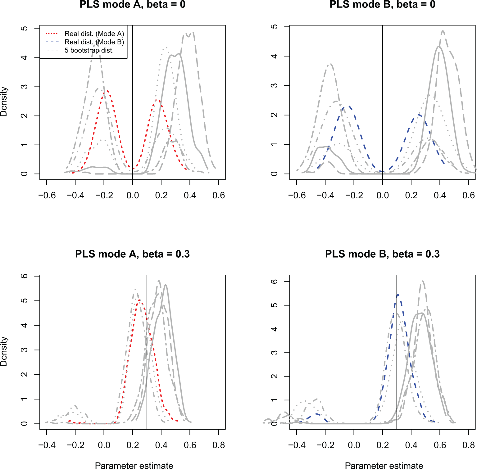
Distribution of parameter estimates over 500 replications and distribution of 500 bootstrap estimates for the first five replications for partial least squares (PLS) Mode A and PLS Mode B in the two-construct model.

Myth 5: PLS Has Minimal Requirements on Sample Size

The belief that PLS does not require a large sample size is widely held. This belief is repeated in 14 of the studies listed in Table 1, and several studies use sample sizes as small as 21 (Cool et al., 1989). The most common citations for the small sample size are two book chapters by Chin (1998; Chin & Newsted, 1999) and the article by Fornell and Bookstein (1982). The arguments presented in these articles can be traced to a single, unpublished conference paper by Wold (partly republished as Wold, 1985a).⁸ However, that paper does not provide any evidence about the statistical power or parameter accuracy of PLS when applied to small samples, but clearly states that PLS parameter estimates converge to their population values only in the theoretical case of “consistency at large” where both the sample size and the number of indicators approach infinity.

In contrast to the lack of support for the myths discussed earlier, a study exists that seeks to provide empirical support for this belief. Chin and Newsted (1999) concluded that PLS generated more accurate parameter estimates than summed scales when the sample size was small. That study has been strongly criticized by Goodhue et al. (2012), who point out that although PLS estimates are slightly larger than regression estimates, so too are standard errors, and there is consequently no advantage in terms of statistical power. However, this result is challenged by a more advanced simulation study by Reinartz et al. (2009). They conclude that although PLS results are always more biased than ML-SEM results, PLS has more statistical power and lower mean estimation error when used with small sample sizes. However, the power estimates in their study are questionable because they are based on p values with an assumption of a t distribution, which we showed earlier to be flawed. Furthermore, their study does not test for false positives, so low p values may be a reflection of positive bias resulting from the use of an inappropriate significance test.

Although the results of these studies show that PLS estimates are on average larger than regression estimates and tend to get larger as the sample size decreases, none of the studies explained why this is the case. We suggest that the apparent advantage of PLS with small sample sizes is a fallacy that results from ignoring the effects of chance correlations. Earlier, we showed that correlated errors bias the PLS path estimates away from zero, leading to artificially inflated path estimates and possibly artificially inflated power. In addition, because the estimates were distinctly different from zero when there was neither an effect between the constructs nor a correlated error in the population (Figure 3), it appears that sampling error is sufficient to substantially distort the parameter estimates from their true value. As sampling error increases with decreasing sample size, there are more chance correlations that PLS can capitalize on; consequently the estimates are biased further from zero.

We illustrate the effect of sample size on PLS parameter estimates by simulating data for our two-construct example using three different sample sizes and either no effect ( $β$ = 0) or a moderate effect ( $β$ = 0.3). Figure 5 shows the probability density distribution of parameter estimates for $β$ for these six conditions. Focusing on the case when $β$ = 0.3, decreasing sample size does not lead to an increase in the accuracy of the parameter estimates but simply an increase in their magnitude, first approaching the population value and then surpassing it as the sample size decreases further. This can also be clearly seen in the results obtained by Chin and Newsted (1999), where the path coefficients are overestimated by up to 40% for the smallest sample size. Thus, we conclude that the small-sample-size capabilities of PLS are a myth arising from ignoring the effect of sampling error amplification and an inappropriate use of the t test for parameter significance.

Figure 5.

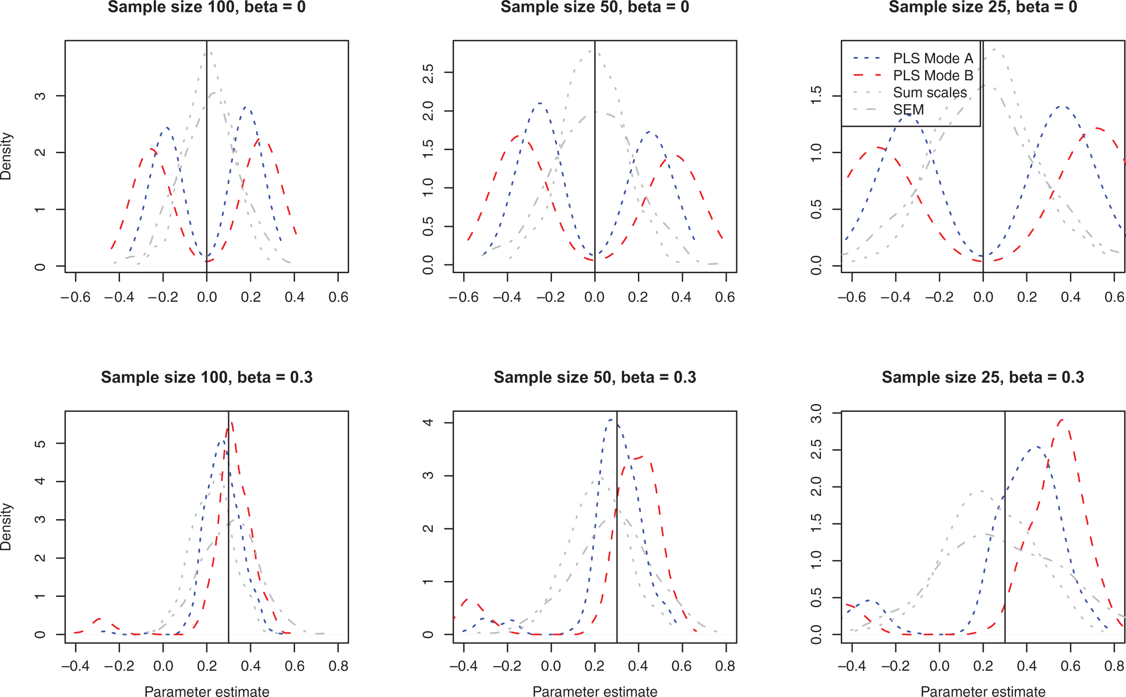
Distribution of parameter estimates for partial least squares (PLS) Mode A, PLS Mode B, summed scales, and structural equation modeling (SEM) with different sample sizes in the two-construct model, 500 replications.

The best remedy for small samples is to collect sufficient data to avoid the problem. SEM techniques for small samples (e.g., Herzog & Boomsma, 2009) and for estimating sample size requirements (e.g., Lai & Kelley, 2011) are actively studied, but fundamental laws of probability limit what can be accomplished. Because the sample size requirement is tied to the size of the model, one way to reduce the required sample size is to reduce the number of indicators by parceling (Landis, Beal, & Tesluk, 2000; Little, Cunningham, Shahar, & Widaman, 2002). Another potentially useful option is to use the limited information 2SLS estimator instead of the full information ML.

Myth 6: PLS Is Most Appropriate for Exploratory or Early Stage Research

When PLS was developed, it was “primarily intended for causal-predictive analysis in situations of high complexity but low theoretical information” (Jöreskog & Wold, 1982, p. 270). In the more recent literature, the notion of low theoretical information has led to the understanding that PLS path modeling is more an exploratory approach than a confirmatory one (Hair et al., 2011).

Using PLS as an exploratory or early-stage theory testing tool does not feature strongly in the early PLS articles. The exception is Lohmöller (1989), who, after comparing PLS and LISREL estimates, concluded correctly that “if [the researcher] is sure that the model is correct,…then he may accept the ML [maximum likelihood SEM] estimates” (p. 213). The corollary assumed by Lohmöller, neither logically implied nor correct, is that PLS is appropriate when the researcher is not sure that the model is correct. Lohmöller nevertheless concludes that “LS methods are…more explorative” (p. 213), implying that the term explorative refers to situations where the model may be incorrect. Similarly, Fornell and Bookstein (1982, p. 450) correctly state that “if one had reason to doubt the accuracy of the theoretical model and/or the validity of the indicators, the LISREL estimate would be exaggerated,” but, like Lohmöller (1989), they erroneously and without evidence conclude that “more credence should be given to the PLS estimate.”

Given that 7 of the studies listed in Table 1 argue for PLS’s suitability for exploratory research, it is problematic that none of the PLS authors explicitly and clearly explain the meaning of the term exploratory or explorative, nor do they explain how PLS supports exploration. In fact, all of the studies listed in Table 1 are presented in a way that is identical to studies applying SEM to test a prespecified model: A literature review is followed by the derivation of causal theory and formal hypotheses and, finally, the estimation of a single model.

One way to understand exploratory analysis is that exploratory methods should reveal patterns in the data (Mulaik, 1985) instead of testing a prespecified hypothesis or model. It is clear that PLS does not have this capability because the model must be completely specified prior to the analysis. Moreover, in contrast to widely used SEM estimators, PLS lacks diagnostic tools such as modification indices that can be used for model building in SEM.

Another way to understand exploratory work is by characterizing it in terms of three features: uncertainty about the correctness of the model, possibly poor measurement, and small sample sizes. However, earlier in this article we concluded that the idea that PLS has special capabilities to handle measurement error and small sample sizes is a myth. We have also demonstrated that PLS cannot be used to test models, that is, to reliably identify model misspecifications. If there is a possibility that the model is incorrect, one should certainly not use a method that cannot detect model misspecification. Finally, construct scores and path estimates calculated using information from an incorrect model are likely to be severely biased (Dijkstra, 1983; Evermann & Tate, 2010). We conclude that because of these weaknesses, PLS is not an appropriate choice for early-stage theory development and testing.

Many introductory texts on SEM describe different model building strategies and show how modification indices can be used for exploration. In addition, new SEM-based methods for exploratory analyses are actively developed (e.g., Asparouhov & Muthén, 2009). If, on the other hand, exploratory research refers to uncertainty about the model rather than the search for a model, we recommend using the 2SLS estimator that is less sensitive to model misspecification than the ML estimator (Bollen, Kirby, Curran, Paxton, & Chen, 2007).

Discussion and Conclusion

In the spirit of Vandenberg (2006), this article has examined statistical myths and urban legends surrounding the often-stated capabilities of the PLS method and its current use in management and organizational research. Tracing back the literature on PLS, we described the origins of each myth to show that they are not based on statistical principles, but misinterpret the original articles on PLS or attribute capabilities to the method based on incorrectly or misleadingly classifying it as an SEM method. We have illustrated why these beliefs are incorrect by using a simple model under conservative conditions (e.g., normal, complete data). Although we acknowledge this limitation, we are not aware of any statistical method that does not work well with a simple model under conservative conditions, but whose performance improves with model complexity. This is counterintuitive, and the PLS literature also makes no such claims. In fact, it often uses the exact same model that we have used (e.g., Chin, 1998). Second, as stated in the introduction, the statistical theory and formal analyses presented in our article do not depend on model complexity.

Despite its demonstrated shortcomings and lack of evidence of the advantages, management researchers increasingly use PLS for purposes that it is not suitable for. One reason that is frequently implicit in the applied literature appears to be a misunderstanding about the relative capabilities of PLS and the commonly used SEM estimators. Our review of several PLS studies shows that authors frequently argue that typical SEM estimators require a large sample size, assume multivariate normality, and have difficulties with some instances of formative indicators. Although some of these assertions were correct in the 1970s when PLS was developed, much has changed since then (Gefen et al., 2011). Nevertheless, the weaknesses of the most commonly used SEM estimators do not imply that PLS is necessarily superior. First, a great many analytical and simulation studies, going back to the early 1970s, have analyzed the behavior of SEM estimators in a wide range of different situations. In contrast, far fewer systematic empirical simulation studies of PLS have been conducted. Hence, comparatively little is understood about PLS, including its weaknesses. However, the absence of a demonstration of unsuitability of a method does not imply suitability of the method. Second, the choice between the typical SEM estimators and PLS is a false dichotomy. If one decides to estimate an SEM model using separate OLS regressions with construct scores, one can rely for guidance on decades of research on how to do this with summed scales or factor scores. In fact, our evidence suggests that even simple summed scales provide better reliability than PLS. When used with regression, these traditional methods to generate composites have test statistics with known distributions allowing NHST. In addition, using a model-based weighting system as used in PLS will guarantee problems with interpretational confounding (Burt, 1976).

If one were a cynic, one could add another reason for the popularity of PLS. Because PLS does not have a test of overall model fit (in contrast to SEM’s test of overall model fit) and its model quality heuristics cannot identify a misspecified model (Evermann & Tate, 2010), researchers who employ PLS never find themselves in a position where a model is decisively rejected by the evidence. Given the publication bias in many fields for “positive” results, it comes as no surprise that some researchers prefer PLS over SEM.

Despite the popularity of PLS, many claims about it must be included among the statistical myths and urban legends. In contrast to Hair et al. (2011), we conclude that PLS is decidedly not a “silver bullet,” and it is very difficult to justify its use for theory testing over SEM or even the more traditional combination of measurement validation with factor analysis and testing hypotheses with regression with summed scales or factor scores. PLS may be useful for purely predictive analyses, but we are not aware of any studies showing this to be the case either.

Footnotes

Declaration of Conflicting Interests

The author(s) declared no potential conflicts of interest with respect to the research, authorship, and/or publication of this article.

Funding

The author(s) received no financial support for the research, authorship, and/or publication of this article.

Notes

References

Aguirre-Urreta

M. I.

Marakas

G. M.

Ellis

M. E.

(in press). Measurement of composite reliability in research using partial least squares: Some issues and an alternative approach. DATA BASE for Advances in Information Systems.

Antonakis

Bendahan

Jacquart

Lalive

(2010). On making causal claims: A review and recommendations. Leadership Quarterly, 21, 1086–1120.

Ashill

N. J.

Jobber

(2010). Measuring state, effect, and response uncertainty: Theoretical construct development and empirical validation. Journal of Management, 36(5), 1278–1308.

Asparouhov

Muthén

(2009). Exploratory structural equation modeling. Structural Equation Modeling: A Multidisciplinary Journal, 16(3), 397–438. doi:10.1080/10705510903008204

Atinc

Simmering

M. J.

Kroll

M. J.

(2011). Control variable use and reporting in macro and micro management research. Organizational Research Methods, 15(1), 57–74.

Avolio

B. J.

Howell

J. M.

Sosik

J. J.

(1999). A funny thing happened on the way to the bottom line: Humor as a moderator of leadership style effects. Academy of Management Journal, 42(2), 219–227. doi:10.2307/257094

Bass

B. M.

Avolio

B. J.

Jung

D. I.

Berson

(2003). Predicting unit performance by assessing transformational and transactional leadership. Journal of Applied Psychology, 88(2), 207–218.

Birkinshaw

Hood

Jonsson

(1998). Building firm-specific advantages in multinational corporations: The role of subsidiary initiative. Strategic Management Journal, 19(3), 221–242.

Birkinshaw

Morrison

Hulland

(1995). Structural and competitive determinants of a global integration strategy. Strategic Management Journal, 16(8), 637–655.

10.

Bollen

K. A.

(1989). Structural equations with latent variables. New York, NY: John Wiley.

11.

Bollen

K. A.

Kirby

J. B.

Curran

P. J.

Paxton

P. M.

Chen

(2007). Latent variable models under misspecification: Two-stage least squares (2SLS) and maximum likelihood (ML) estimators. Sociological Methods & Research, 36(1), 48–86. doi:10.1177/0049124107301947

12.

Bollen

K. A.

Stine

R. A.

(1992). Bootstrapping goodness-of-fit measures in structural equation models. Sociological Methods & Research, 21(2), 205–229. doi:10.1177/0049124192021002004

13.

Burt

R. S.

(1976). Interpretational confounding of unobserved variables in structural equation models. Sociological Methods & Research, 5(1), 3–52. doi:10.1177/004912417600500101

14.

Cheung

M.-S.

Myers

M. B.

Mentzer

J. T.

(2011). The value of relational learning in global buyer-supplier exchanges: A dyadic perspective and test of the pie-sharing premise. Strategic Management Journal, 32(10), 1061–1082. doi:10.1002/smj.926

15.

Chin

W. W.

(1998). The partial least squares approach to structural equation modeling. In Marcoulides

G. A.

(Ed.), Modern methods for business research (pp. 295–336). Mahwah, NJ: Lawrence Erlbaum.

16.

Chin

W. W.

Newsted

P. R.

(1999). Structural equation modeling analysis with small samples using partial least squares. Statistical Strategies for Small Sample Research, 2, 307–342.

17.

Cohen

West

S. G.

Aiken

L. S.

(2003). Applied multiple regression/correlation analysis for the behavioral sciences. London, England: Lawrence Erlbaum.

18.

Cool

Dierickx

Jemison

(1989). Business strategy, market structure and risk-return relationships: A structural approach. Strategic Management Journal, 10(6), 507–522.

19.

Cording

Christmann

King

D. R.

(2008). Reducing causal ambiguity in acquisition integration: Intermediate goals as mediators of integration decisions and acquisition performance. Academy of Management Journal, 51(4), 744–767.

20.

Crossland

Hambrick

D. C.

(2011). Differences in managerial discretion across countries: How nation-level institutions affect the degree to which CEOs matter. Strategic Management Journal, 32(8), 797–819. doi:10.1002/smj.913

21.

Delios

Beamish

P. W.

(1999). Geographic scope, product diversification and the corporate performance of Japanese firms. Strategic Management Journal, 20(8), 711–727.

22.

Dijkstra

T. K.

(1983). Some comments on maximum likelihood and partial least squares methods. Journal of Econometrics, 22(1-2), 67–90.

23.

Duxbury

L. E.

Higgins

C. A.

(1991). Gender differences in work-family conflict. Journal of Applied Psychology, 76(1), 60–73. doi:10.1037/0021-9010.76.1.60

24.

Echambadi

Campbell

Agarwal

(2006). Encouraging best practice in quantitative management research: An incomplete list of opportunities. Journal of Management Studies, 43(8), 1801–1820. doi: 10.1111/j.1467-6486.2006.00660.x

25.

Edwards

J. R.

(2011). The fallacy of formative measurement. Organizational Research Methods, 14(2), 370–388. doi:10.1177/1094428110378369

26.

Evermann

Tate

(2010). Testing models or fitting models? Identifying model misspecification in PLS. In ICIS 2010 proceedings. Retrieved from http://aisel.aisnet.org/icis2010_submissions/21

27.

Fornell

Bookstein

F. L.

(1982). Two structural equation models: LISREL and PLS applied to consumer exit-voice theory. Journal of Marketing Research, 19(4), 440–452.

28.

Fornell

Larcker

D. F.

(1981). Evaluating structural equation models with unobservable variables and measurement error. Journal of Marketing Research, 18(1), 39–50.

29.

Gefen

Rigdon

E. E.

Straub

D. W.

(2011). An update and extension to SEM guidelines for administrative and social science research. MIS Quarterly, 35(2), iii–xiv.

30.

Goodhue

D. L.

Lewis

Thompson

(2012). Comparing PLS to regression and LISREL: A response to Marcoulides, Chin, and Saunders. MIS Quarterly, 36(3), 703–716.

31.

Groth

Hennig-Thurau

Walsh

(2009). Customer reactions to emotional labor: The roles of employee acting strategies and customer detection accuracy. Academy of Management Journal, 52(5), 958–974.

32.

Gruber

Heinemann

Brettel

Hungeling

(2010). Configurations of resources and capabilities and their performance implications: An exploratory study on technology ventures. Strategic Management Journal, 31(12), 1337–1356.

33.

Hair

J. F.

Ringle

C. M.

Sarstedt

(2011). PLS-SEM: Indeed a silver bullet. Journal of Marketing Theory & Practice, 19(2), 139–152. doi:10.2753/MTP1069-6679190202

34.

Hair

J. F.

Sarstedt

Pieper

T. M.

Ringle

C. M.

(2012). The use of partial least squares structural equation modeling in strategic management research: A review of past practices and recommendations for future applications. Long Range Planning, 45(5–6), 320–340. doi:10.1016/j.lrp.2012.09.008

35.

Henseler

Chin

W. W.

(2010). A comparison of approaches for the analysis of interaction effects between latent variables using partial least squares path modeling. Structural Equation Modeling: A Multidisciplinary Journal, 17(1), 82–109. doi:10.1080/10705510903439003

36.

Henseler

Sarstedt

(2013). Goodness-of-fit indices for partial least squares path modeling. Computational Statistics. doi:10.1007/s00180-012-0317-1

37.

Herzog

Boomsma

(2009). Small-sample robust estimators of noncentrality-based and incremental model fit. Structural Equation Modeling: A Multidisciplinary Journal, 16(1), 1–27. doi:10.1080/10705510802561279

38.

Howell

J. M.

Avolio

B. J.

(1993). Transformational leadership, transactional leadership, locus of control, and support for innovation: Key predictors of consolidated-business-unit performance. Journal of Applied Psychology, 78(6), 891–902. doi:10.1037/0021-9010.78.6.891

39.

Howell

J. M.

Hall-Merenda

K. E.

(1999). The ties that bind: The impact of leader-member exchange, transformational and transactional leadership, and distance on predicting follower performance. Journal of Applied Psychology, 84(5), 680–694.

40.

Bentler

P. M.

(1999). Cutoff criteria for fit indexes in covariance structure analysis: Conventional criteria versus new alternatives. Structural Equation Modeling: A Multidisciplinary Journal, 6(1), 1–55.

41.

Hulland

(1999). Use of partial least squares (PLS) in strategic management research: A review of four recent studies. Strategic Management Journal, 20(2), 195–204.

42.

Johansson

J. K.

Yip

G. S.

(1994). Exploiting globalization potential: U.S. and Japanese strategies. Strategic Management Journal, 15(8), 579–601.

43.

Jöreskog

K. G.

Wold

(1982). The ML and PLS techniques for modeling with latent variables. In Jöreskog

K. G.

Wold

(Eds.), Systems under indirect observation: Causality, structure, prediction (pp. 263–270). Amsterdam, the Netherlands: North-Holland.

44.

Lai

Kelley

(2011). Accuracy in parameter estimation for targeted effects in structural equation modeling: Sample size planning for narrow confidence intervals. Psychological Methods, 16(2), 127–148. doi:10.1037/a0021764

45.

Landis

R. S.

Beal

D. J.

Tesluk

P. E.

(2000). A comparison of approaches to forming composite measures in structural equation models. Organizational Research Methods, 3(2), 186–207. doi:10.1177/109442810032003

46.

Lehmann

Casella

(1998). Theory of point estimation. New York, NY: Springer.

47.

Little

T. D.

Cunningham

W. A.

Shahar

Widaman

K. F.

(2002). To parcel or not to parcel: Exploring the question, weighing the merits. Structural Equation Modeling, 9(2), 151–173.

48.

Lohmöller

J. B.

(1989). Latent variable path modeling with partial least squares. Heidelberg, Germany: Physica-Verlag.

49.

McDonald

R. P.

(1996). Path analysis with composite variables. Multivariate Behavioral Research, 31(2), 239–270.

50.

Meznar

M. B.

Nigh

(1995). Buffer or bridge? Environmental and organizational determinants of public affairs activities in American firms. Academy of Management Journal, 38, 975–996.

51.

Mulaik

S. A.

(1985). Exploratory statistics and empiricism. Philosophy of Science, 52(3), 410–430.

52.

Nickerson

R. S.

(2000). Null hypothesis significance testing: A review of an old and continuing controversy. Psychological Methods, 5(2), 241–301. doi:10.1037//1082-989X.5.2.241

53.

Nunnally

(1978). Psychometric theory. New York, NY: McGraw-Hill.

54.

Olk

Young

(1997). Why members stay in or leave an R&D consortium: Performance and conditions of membership as determinants of continuity. Strategic Management Journal, 18(11), 855–877.

55.

Peng

D. X.

Lai

(2012). Using partial least squares in operations management research: A practical guideline and summary of past research. Journal of Operations Management, 30(6), 467–480. doi:10.1016/j.jom.2012.06.002

56.

Raykov

(1997). Estimation of composite reliability for congeneric measures. Applied Psychological Measurement, 21(2), 173–184. doi:10.1177/01466216970212006

57.

Reinartz

W. J.

Haenlein

Henseler

(2009). An empirical comparison of the efficacy of covariance-based and variance-based SEM. International Journal of Research in Marketing, 26(4), 332–344. doi:10.1016/j.ijresmar.2009.08.001

58.

Robins

J. A.

Tallman

Fladmoe-Lindquist

(2002). Autonomy and dependence of international cooperative ventures: An exploration of the strategic performance of U.S. ventures in Mexico. Strategic Management Journal, 23(10), 881–901. doi:10.1002/smj.260

59.

Rosseel

(2012). Lavaan: An R package for structural equation modeling. Journal of Statistical Software, 48(2), 1–36.

60.

Sanchez

Trinchera

(2012). plspm version 0.2-2 [Computer software]. Retrieved from http://cran.r-project.org/web/packages/plspm/index.html

61.

Sarkar

M. B.

Echambadi

R. A. J.

Harrison

J. S.

(2001). Alliance entrepreneurship and firm market performance. Strategic Management Journal, 22(6/7), 701–711. doi:10.1002/smj.179

62.

Shamir

Zakay

Breinin

Popper

(1998). Correlates of charismatic leader behavior in military units: Subordinates’ attitudes, unit characteristics, and superiors’ appraisals of leader performance. Academy of Management Journal, 41, 387–409.

63.

Shea

C. M.

Howell

J. M.

(2000). Efficacy-performance spirals: An empirical test. Journal of Management, 26(4), 791–812. doi:10.1177/014920630002600409

64.

Sosik

J. J.

Avolio

B. J.

Kahai

S. S.

(1997). Effects of leadership style and anonymity on group potency and effectiveness in a group decision support system environment. Journal of Applied Psychology, 82(1), 89–103.

65.

Sosik

J. J.

Kahai

S. S.

Piovoso

M. J.

(2009). Silver bullet or voodoo statistics? A primer for using the partial least squares data analytic technique in group and organization research. Group & Organization Management, 34(1), 5–36. doi:10.1177/1059601108329198

66.

Tiwana

(2008). Do bridging ties complement strong ties? An empirical examination of alliance ambidexterity. Strategic Management Journal, 29(3), 251–272.

67.

Tsang

E. W. K.

(2002). Acquiring knowledge by foreign partners from international joint ventures in a transition economy: Learning-by-doing and learning myopia. Strategic Management Journal, 23(9), 835–854. doi:10.1002/smj.251

68.

Vandenberg

R. J.

(2006). Introduction: Statistical and methodological myths and urban legends. Organizational Research Methods, 9(2), 194–201. doi:10.1177/1094428105285506

69.

Vinzi

V. E.

Chin

W. W.

Henseler

Wang

(2010). Editorial: Perspectives on partial least squares. In Vinzi

V. E.

Chin

W. W.

Henseler

Wang

(Eds.), Handbook of partial least squares (pp. 1–22). Berlin, Germany: Springer.

70.

Wang

Bansal

(2012). Social responsibility in new ventures: Profiting from a long-term orientation. Strategic Management Journal, 33, 1135–1153. doi:10.1002/smj.1962

71.

Wold

(1985a). Factors influencing the outcome of economic sanctions. Trabajos de Estadistica y de Investigacion Operativa, 36(3), 325–338. doi:10.1007/BF02888567

72.

Wold

(1985b). Systems analysis by partial least squares. In Nijkamp

Leitner

Wrigley

(Eds.), Measuring the unmeasurable (pp. 221–252). Dordrecht, Germany: Marinus Nijhoff.

73.

Wood

(2005). Bootstrapped confidence intervals as an approach to statistical inference. Organizational Research Methods, 8(4), 454–470. doi:10.1177/1094428105280059

74.

Zimmerman

D. W.

Williams

R. H.

(1977). The theory of test validity and correlated errors of measurement. Journal of Mathematical Psychology, 16(2), 135–152.

75.

Zott

Amit

(2008). The fit between product market strategy and business model: Implications for firm performance. Strategic Management Journal, 29(1), 1–26.