Data Sparseness and Variance in Accounting Profitability

Abstract

A central question in strategic management is why some firms perform better than others. One approach to addressing this question empirically is to decompose the variance in firm-level profitability into firm, industry, location, and year components. Although it is well established that data sparseness in variance decomposition studies can lead to overestimating particular variance components, little attention has been paid to sample size requirements in strategic management studies that have examined the nature of differences in firm profitability. We conduct a meta-regression and variance decomposition study and conclude that the variation in the results from previous studies is driven—to a considerable extent—by the number of observations per group within a component. Based on these findings, we draw conclusions regarding the validity and reliability of previous variance decomposition studies and provide implications for current debates in the strategic management literature.

Keywords

firm profitability variance decomposition data sparseness meta-analysis

Introduction

In strategic management, variance decomposition analysis has frequently been employed to examine why some firms perform better than others. Since the mid 1980s, numerous studies have addressed the extent to which industry, location, and year effects explain variances in accounting profitability (e.g., Chan, Makino, & Isobe, 2010; Goddard, Tavakoli, & Wilson, 2009; Goldszmidt, Brito, & De Vasconcelos, 2011; Hawawini, Subramanian, & Verdin, 2003, 2004; Hough, 2006; Karniouchina, Carson, Short, & Ketchen, 2013; Ketelhöhn & Quintanilla, 2012; Ma, Tong, & Fitza, 2013; Makino, Isobe, & Chan, 2004; McGahan, 1999; McGahan & Porter, 1997, 2002; McGahan & Victer, 2010; Roquebert, Phillips, & Westfall, 1996; Rumelt, 1991; Schmalensee, 1985; Short, Ketche, Palmer, & Hult, 2007). Variance decomposition analysis offers a straightforward way to assess contextuality or the extent to which there is a link between the macro (industry, region, and year) and micro (firm) levels. Although variance decomposition analysis is mainly a descriptive tool, it provides insights into the relative importance of the external environment of a firm or to what extent industry, location, or year effects matter for the performance of firms compared with a firm-specific characteristics. Applying variance decomposition analysis to the study of accounting profitability begins from the simple observation that firms that share the same external environment (location, industry, and year) are more similar in their performance than firms that do not share the same external environment. In this fashion, we can better assess the extent to which variance in accounting profitability across firms can be attributed to between-firm variance, between-industry variance, between-location variance, and/or between-year variance (McGahan & Porter, 1997). Although firm-level effects are the most important class of effects utilized in the literature to explain variations in accounting profitability, the generally accepted tendency in scholarly research acknowledges that the external environment of the firm matters.

Whereas the early empirical literature focused primarily on the extent to which industry effects have driven the variance in firm profitability, more recent studies have turned their attention to the importance of location. Simultaneously, variance decomposition studies have increasingly moved toward estimating more complex data structures by using more fine-grained classifications of industries (e.g., industry sectors instead of industry groups) and locations (e.g., subregions within nations instead of nations). Likewise, research has increasingly focused on the extent to which industry effects are contingent on year and location, which provides a more explicit link with other strands of research in strategic management, organization studies, and business, such as the literature on industry life cycles (e.g., Klepper, 1997) and regional clusters (e.g., Porter, 1998). McGahan and Porter (2002) indicated that these more complex model structures are necessary because using broad industry and location taxonomies obscures the variation within these classifications and might lead to incorrect inferences regarding the relationship between a firm’s environment and its accounting profitability.

Parallel to these developments, however, variance decomposition studies remain ambiguous about the importance of a firm’s external environment for explaining variances in accounting profitability. For example, the industry effect regarding the return on assets (ROA) ranges from less than 1% (Chen & Lin, 2006) to over 31% (McGahan, 1999), whereas the country effect varies from 2% (Hawawini et al., 2004) to 22% (McGahan & Victer, 2010). This naturally raises the question as to why there is such a range of magnitude in which the highest industry and country effects are more than 10 times the size of the lowest values.

Naturally, differences in the relative importance of firms’ external environments across studies can be attributed to differences in institutional settings, industry classifications, types of firms in the sample, empirical methods employed, and the time period under study (McGahan & Porter, 2002). In this article, however, we argue that at least part of the differences reported across studies can be attributed to data sparseness in some of the empirical strategic management studies, which can result in the inflation of variance components. Data sparseness in variance decomposition studies describes the situation in which there are limited numbers of observations per group within a certain component (e.g., the number of observations per industry sector), which typically yields overestimations for such variance components (Clarke & Wheaton, 2007; Maas & Hox, 2004; Snijders & Bosker, 1993). Despite concerns about sample size in the study of multilevel phenomena in related subfields within strategic management, organization studies, and business studies (e.g., Peterson, Arregle, & Martin, 2012), to the best knowledge of the authors, few scholars have addressed data sparseness problems in variance decomposition studies that have examined firm profitability in the field of strategic management. Although informed strategy and business scholars are aware that sparse samples within components can bias outcomes, we argue that many studies that have examined variance in accounting profitability utilize sample sizes that are inadequate for conducting a proper variance decomposition analysis. In turn, this approach could have resulted in overestimations and exaggerations of the relative importance of firms’ industry and location in the strategic management literature. Thus, our study adds to one of the key debates in the strategic management literature, namely, whether differences in firm performance can be predominantly attributed to differences in resources, capabilities, and organizational forms across firms (i.e., the resource-based view; see Barney, 1991; Peteraf, 1993; Wernerfelt, 1984) or to industry and external market organization (i.e., the market-based view; see Bain, 1968; Porter, 1980).

The purpose of this study is to generate evidence regarding how substantial the problem of data sparseness is in the strategic management literature on accounting profitability. First, we conduct a meta-analysis that examines the extent to which the variation in industry effects that has been found can be attributed to data sparseness. In this context, we also provide an assessment of which variance decomposition studies are more meaningful in that they are not subject to data sparseness problems. Second, we use a variance decomposition study on accounting profitability in three southern European countries (France, Italy, and Spain) and ascertain that the data sparseness problem can result (in some cases) in an inflation of certain variance components.

The Problem: Data Sparseness and Variance Decomposition

Since the seminal work of Schmalensee (1985) and McGahan and Porter (1997), variance decomposition has been used to study the relative importance of industry, location, year, and firm-specific effects on firm profitability.¹ Applying variance decomposition to empirical work on firm profitability begins with the simple observation that firms that share, for example, the same industry or location are more alike in their performance than firms that do not share these features because of the common environment to which they belong. By measuring the extent to which different firms that share the same group(s) have similar profitability compared with the profitability of firms in different group(s), we can assess the extent to which variance in firm profitability can be attributed to between-firm variance, between–corporate parent variance, between-industry variance, or between-location variance. As noted by several scholars, the variance decomposition literature is predominantly descriptive in nature, and the technique provides no information about the determinants of firm profitability.

In the previous empirical literature, several estimation methods have been used to decompose the variance in accounting profitability, most notably the nested analysis of variance (nested ANOVA), components of variance (COV), and mixed hierarchical and cross-classified or multilevel models. Although sample size requirements have also been discussed in the context of the ANOVA and COV (see e.g., Bliese & Halverson, 1998; Bonett, 2002),² the most recent literature on data sparseness and variance estimation has predominantly focused on mixed hierarchical and cross-classified models. However, it is important to note that data sparseness is a concern regardless of the estimation method, although some scholars argue that the problem is of greater concern for ANOVA and COV than for multilevel analysis (Bou & Satorra, 2010). With ANOVA, a small number of observations per group typically results in a violation of the assumption of the normal distribution of the dependent variable within each group and the equality of variances of each group. At the same time, multilevel analysis requires a large number of groups (Bou & Satorra, 2010). For a detailed discussion on the topic, the reader can refer to the work of Bou and Satorra (2010).

Because the estimation methods for the ANOVA, COV, and mixed hierarchical and cross-classified models are asymptotic, the sample size must be sufficiently large, which means that there must be a sufficient number of observations (particularly at the higher levels of analysis) and a sufficient number of observations per group within components. Within the context of studies that examine variance in accounting profitability, this indicates not only that the number of industries, locations, and groups within other classifications must be sufficiently large but also that there must be a sufficient number of firms per group. Although there is no official rule, rules of thumb in the literature recommend a minimum of 10 to 30 observations per group within each component (Bryk & Raudenbush, 1992; Hox, 2010; Kreft & De Leeuw, 1998; Maas & Hox, 2004). When there are many groups within a certain component with few observations or only one observation, there is limited variance within groups, which means that the individual and group levels are rather indistinguishable.³ Likewise, the different group levels and particularly the interaction effects between the group levels (e.g., industry-by-region or industry-by-year effects) become less distinguishable as well. In turn, small group sizes in combination with differences across individuals yield results with inflated higher-level variance components. In such cases, the use of ANOVA and COV even poses additional problems in that these methods tend to assign shared variance to only one of the effects entered in the analysis, resulting in a severe inflation of one of the effects (Bou & Satorra, 2010; Hough, 2006).

In general, simulation studies that have examined the effect of sample and group size on variance estimates using mixed hierarchical and cross-classified models have shown that variance decomposition analysis functions poorly with small sample sizes, particularly when group sizes are very small (<5 observations per group) (Bell, Ferron, & Kromrey, 2008; Clarke, 2008; Maas & Hox, 2004; Moineddin, Matheson, & Glazier 2007; Thell et al., 2011). Although most simulation studies have been conducted for models with only two levels (e.g., only firms and industries), Clarke and Wheaton (2007) argued that data sparseness is even more problematic when estimating more complicated models that include three or more levels and interactions between the levels (i.e., cross-classified models) because group size for these classifications is frequently small.

A Meta-Regression of Variance Decomposition Studies on Accounting Profitability

Although the problem of data sparseness has received little or no attention in variance decomposition studies on firm profitability, this does not indicate that these studies do not face similar problems. Early variance decomposition studies that focused primarily on industry effects (e.g., Chang & Singh, 2000; Kessides, 1990; Mauri & Michaels, 1998; Rumelt, 1991; Schmalensee, 1985) worked with samples with two firms per industry on average. In fact, in our assessment of an inventory of variance decomposition studies that have examined the industry effect on ROA (among other issues), we discovered that more than 50% of the studies utilize on average fewer than 10 firms per industry in their estimations, and 20% of the studies use fewer than 5 firms per industry (see Table 1); positive outliers include the studies by Short et al. (2007), Goddard et al. (2009), Bou and Satorra (2010), Goldzsmidt et al. (2011), and Diaz Hermelo and Vassolo (2012). A quick survey of the results reported in these studies displayed in Table 1 shows that the unconditional correlation between the average industry effect reported in the studies and the natural logarithm of the average number of firms per industry is approximately –0.13; thus, the smaller the average number of firms per industry is, the higher the industry effect (see Figure 1).

Figure 1.

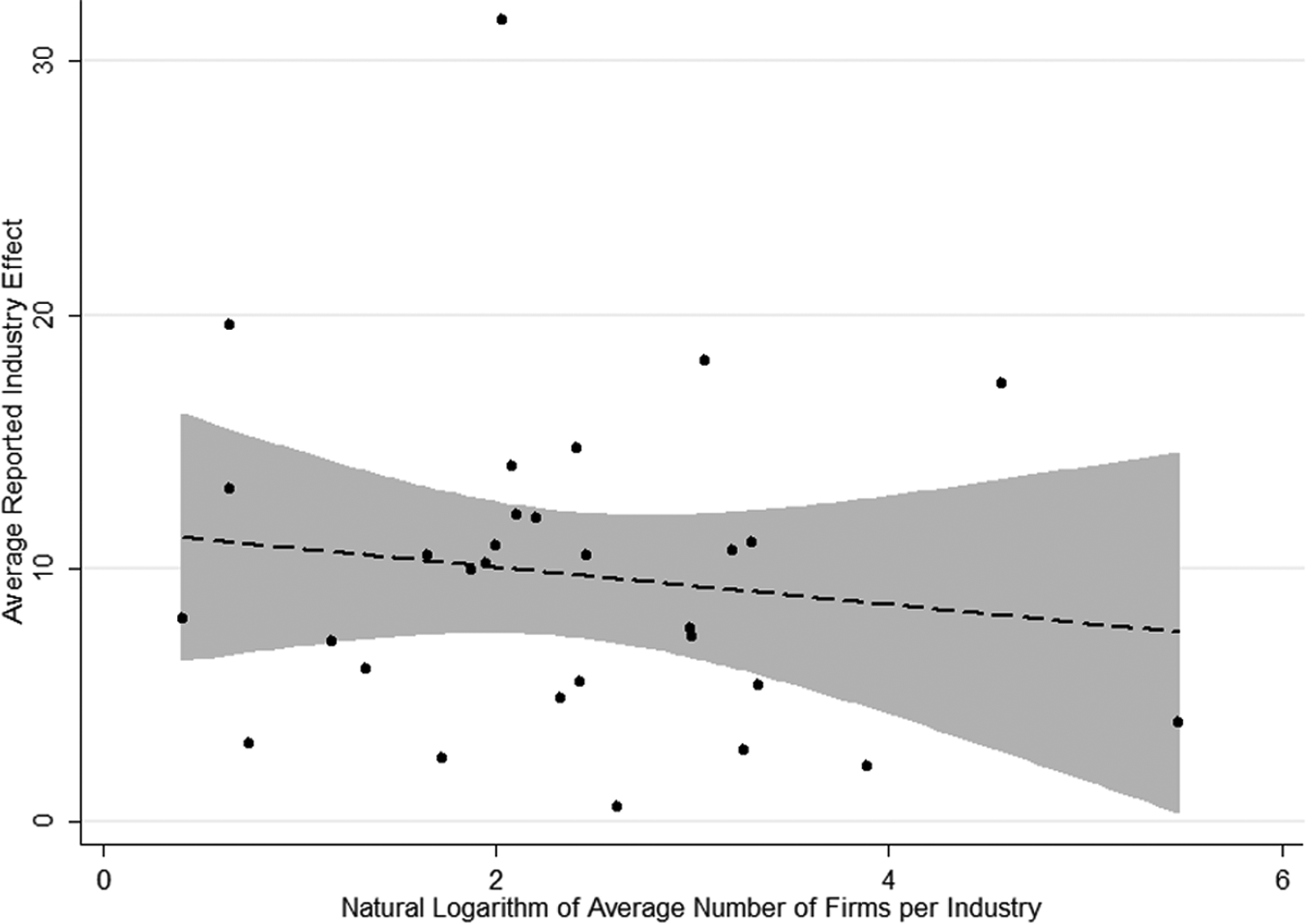
Average reported industry effects versus average number of firms per industry in variance decomposition studies.

Table 1.

Overview of Studies Included in the Meta-Analysis.

Study	Years of Coverage	Average Reported Industry Effect	Average Firm-Industry Ratio
Brito and Vasconcelos (2006)	1997-2001	5.4	28.1
Chan, Makino, and Isobe (2010)	1996-2005	10.7	24.6
Chang and Hong (2002)	1985-1996	10.9	7.4
Chen and Lin (2006)	1998-2003	0.6	13.7
Claver, Molina, and Tari (2002)	1994-1998	2.5	5.6
Diaz Hermelo and Vassolo (2012)	1990-2006	2.8	26.0
Fidalgo and Victoria (2002)	1991-1994	5.5	11.3
Goddard, Tavakoli, and Wilson (2009)	1992-2000	3.9	239.1
Goldszmidt, Brito, and De Vasconcelos (2011)	1995-2004	2.2	48.9
Hawawini, Subramanian, and Verdin (2003)	1987-1996	12.1	8.2
Hough (2006)	1995-1999	9.9	6.5
Karniouchina, Carson, Short, and Ketchein (2013)	1979-1994	7.3	20.0
Ketelhöhn and Quintanilla (2012)	2000-2004	14.0	8.0
Lieu and Chi (2006)	1994-2000	3.1	2.1
Ma, Tong, and Fitza (2013)	1998-2001	8.0	1.5
Makino, Isobe, and Chan (2004)	1996-2001	7.1	3.2
Mauri and Michaels (1998)	1978-1992	6.0	3.8
McGahan (1999)	1981-1994	31.6	7.6
McGahan and Porter (1997)	1981-1994	14.7	11.1
McGahan and Porter (2002)	1985-1991	10.5	11.7
McGahan and Victer (2010)	1993-2003	12.0	9.1
McNamara, Aime, and Vaaler (2005)	1987-1996	11.0	27.08
Misangyi, Elms, Greckhamer, and Lepine (2006)	1984-1999	7.6	19.9
Roquebert, Phillips, and Westfall (1996)	1985-1991	10.2	7.0
Rumelt (1991)	1974-1977	13.1	1.9
Schmalensee (1985)	1975	19.6	1.9
Short, Ketchen, Palmer, and Hult (2007)	1993-1997	17.3	97.1
Short, McKelvie, Ketchen, and Chandler (2009)	1994-1999	18.2	21.4
Tarziján and Ramirez (2011)	1998-2007	10.5	5.2
Tong, Alessandri, Reuer, and Chintakananda, (2008)	1997-1999	4.9	10.3

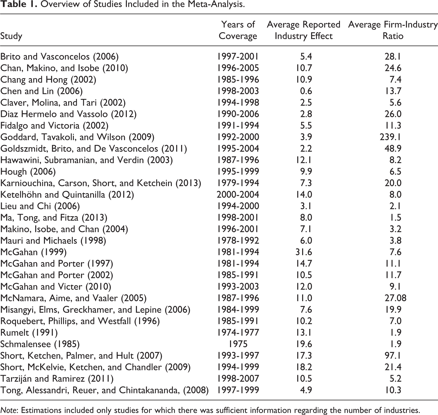
Note: Estimations included only studies for which there was sufficient information regarding the number of industries.

Although we indeed observe a negative relationship between the average reported industry effect and average number of firms per industry examined in studies, we must consider that there are considerable differences across studies regarding institutional settings, classifications of industries, types of firms in the samples, empirical methods employed, the time period under study, and the number of components that are included. Thus, we conduct a meta-analysis to examine the extent to which differences in industry effects reported in studies are driven by data sparseness. Please note that although the problem of data sparseness in variance decomposition studies is not limited to industry effects, we focus our meta-analysis on these effects because (a) the variance decomposition literature on accounting profitability has traditionally focused predominantly on industry effects, and (b) there are still an insufficient number of studies to conduct a meta-analysis on, for example, location effects.

The objective of meta-analyses is to synthesize and explain variations in previous research findings by means of a statistical analysis of a large collection of results from individual studies (Glass, 1976). The variance in effects reported across studies could be explained by (a) differences in methodology and (b) structural differences across subpopulations. In light of this study, this proposition is valuable because it could tell us which characteristics of the underlying variance decomposition study are truly important for determining the differences in the magnitude of the industry effects across studies. The meta-analysis could tell us, for example, whether studies with a smaller number of observations per industry yield larger industry effects, holding other study aspects constant.

Selection of Studies

To examine the influence of data sparseness on the industry effects found in studies, we constructed a database with industry effects reported in different studies. To acquire a systematic and representative set of journal articles, we used Google Scholar to select all articles that cited either Schmalensee (1985) or McGahan and Porter (1997). Using the keywords industry effects, firm profitability, and variance decomposition, this approach resulted in a set of 170 studies for the 1985-2013 period. Following the snowballing technique introduced by De Groot, Poot, and Smit (2009), we carefully scanned the references of all of the journal articles and book chapters in the sample (working papers were excluded from our analysis). Subsequently, we went through all of the articles and included only those estimates that (a) adopted a variance decomposition approach; (b) used ROA, return on invested capital (ROIC), return on equity (ROE), or profit margin (PM) as the output indicator; (c) included sufficient information regarding their study design and empirical strategy; and (d) did not focus on specific subsectors (although estimates for broad sectors, such as manufacturing and services, were included). Most notably, a number of studies were omitted because no information was provided regarding the number of observations per industry. In total, 30 journal articles and book chapters were found that fulfilled the criteria to a sufficient degree, which provided us with 119 different estimates. These estimates show considerable variation in the magnitude of the industry effects found. Table 1 provides information regarding the studies included, the average industry effect found in each study, and the average number of observations per industry.

Variables in the Meta-Regression

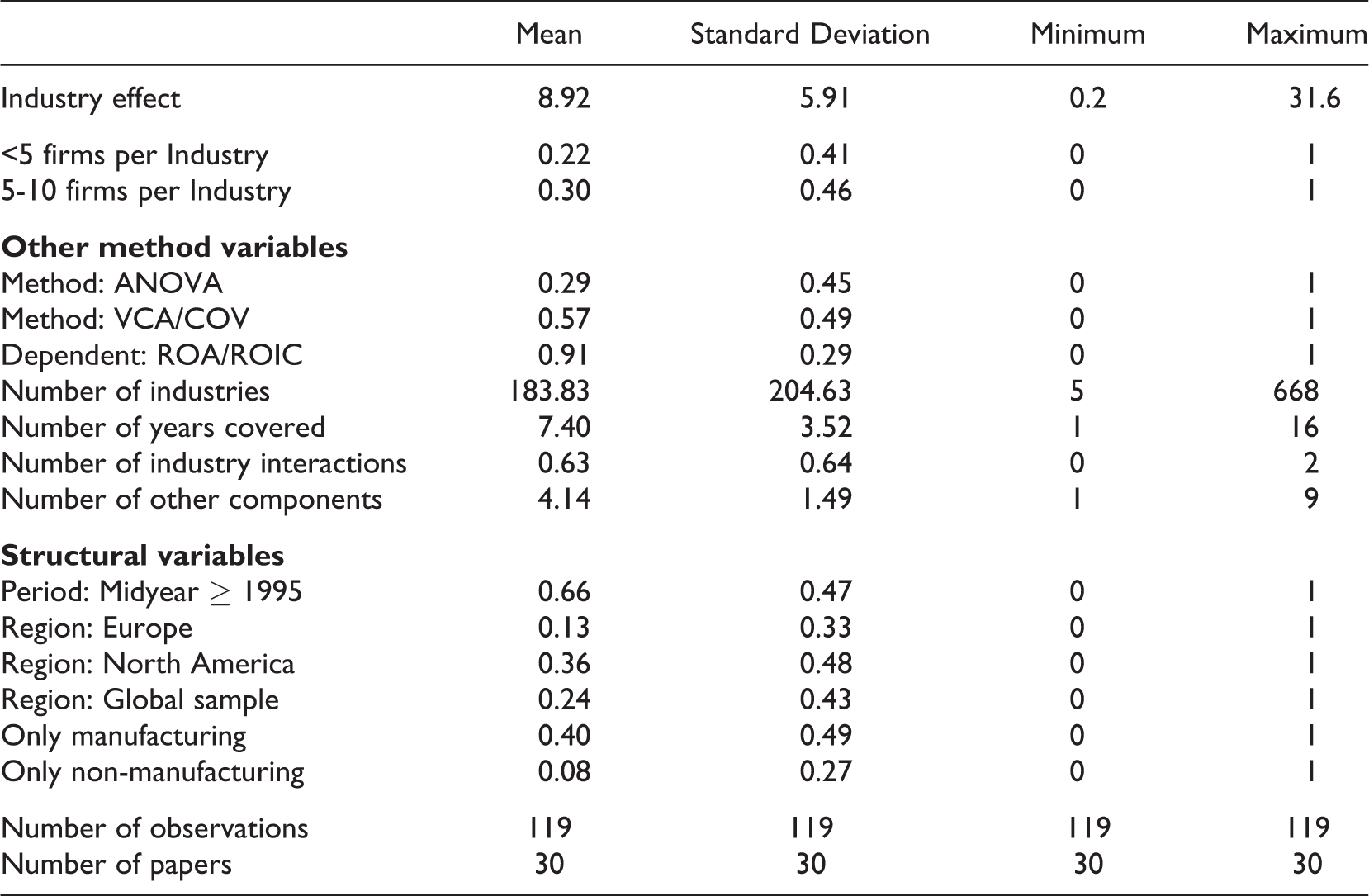
To examine the effect of data sparseness on the reported industry effect, we include two dummy variables. The Boolean dummy variable <5 firms per industry takes the value of 1 if the number of firms per industry in the estimation is less than 5, whereas the Boolean dummy variable 5 to 10 firms per industry takes the value of 1 if the number of firms per industry in the estimation is between 5 and 10. These cutoff points are based on (a) findings from simulation studies that concluded that variance decomposition analysis functions poorly when group sizes are very small (<5 observations per group) and (b) the rule of thumb from the multilevel analysis literature that recommends at least 10 observations per group (see the previous section). Based on the outcomes from simulation studies (Bell et al., 2008; Clarke, 2008; Maas & Hox, 2004; Moineddin et al., 2007; Thell et al., 2011), we expect an inflation of the industry effect when the average number of firms per industry is very low.

In addition, we add control variables that might confound the relationship between the number of firms per industry and the reported industry effect. As indicated previously, it is likely that industry effects result from (a) method heterogeneity and (b) structural heterogeneity (cf. Disdier & Head, 2008). Method heterogeneity originates from differences in statistical techniques and study design. First, variance decomposition studies differ in the statistical techniques they have applied. As noted by Hough (2006) and Bou and Satorra (2010), ANOVA and COV are heavily contested due to their inability to address collinearity among different components, which can result in overestimated industry effects.⁴ More recently, multilevel analysis has been used to address these issues and generally reports lower industry effects and higher firm effects (e.g., Hough, 2006). In our analysis, we compare the relationship between statistical techniques (ANOVA, COV, or multilevel and other methods) and the reported industry effect. Second, studies can differ in terms of the profitability indicator that is used. Although most studies use ROA as their profitability indicator, some have used ROIC or return sales (ROS) as performance measures. Third, variance decomposition studies can differ regarding the number of dimensions included. Most importantly, the number of components included in the analyses has increased over time in that recent studies have focused on location effects and industry interaction effects (industry-by-country, industry-by-subregion, and industry-by-year effects). Here, it can be expected that the more other components and the more industry interaction effects that are included in an analysis, the lower the industry effect that is reported. Likewise, studies differ regarding the industrial classification used and the years of coverage. Because these aspects can confound the relationship between data sparseness and the reported industry effect, we control for these effects.

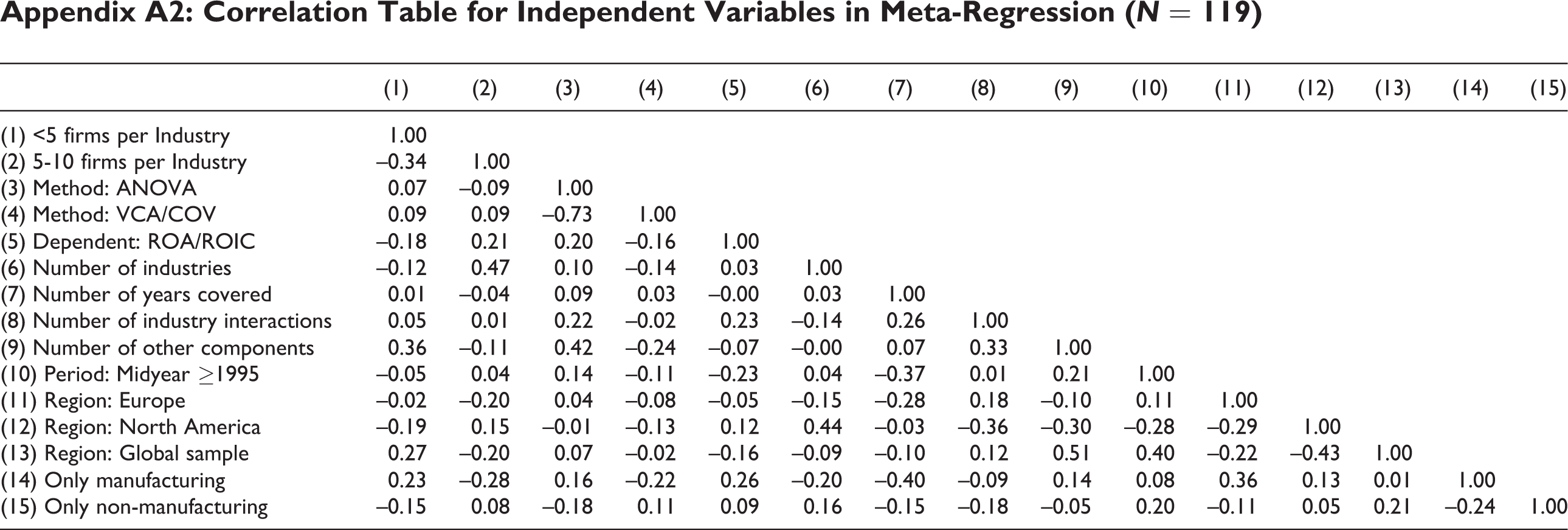
With respect to structural heterogeneity, industry effects do not necessarily have to be identical across subpopulations. In this analysis, we include information regarding the midyear for the sample in which the study was conducted (before or after 1995), the countries covered (global sample, Europe, North America, or a particular country or continent in the rest of the world), and the industries covered (all industries, only manufacturing industries, or only non–manufacturing industries). Descriptive statistics and a correlation table of the variables included in the model are provided in Appendix A1 and Appendix A2, respectively.

Meta-Regression Results

To analyze the effect of data sparseness on the magnitude of the industry effects found in prior studies, we follow the meta-analysis literature (e.g., DerSimonian & Laird, 1986; Disdier & Head, 2008; Jeppensen, List, & Folmer, 2002) and estimate the following simple reduced form of random-effects meta-regression:

I N D_{i j} = α_{0} + α_{1} O I_{i j} + α_{2} X_{i j} + u_{i} + e_{i j},

where $I N D_{i j}$ is the jth industry effect reported in article i, $O I_{i j}$ is a set of dummy variables capturing the number of observations per industry, $X_{i j}$ is a set of meta-independent variables that are thought to have an impact on the reported industry effect, and $u_{i}$ are the random-article effects. As noted by Jeppensen et al. (2002), the random effects control for the commonality of the dependence of observations within each paper by treating estimates from the same paper as distinct but possibly correlated observations in the meta-regression.⁵ Compared with the traditional ordinary least squares (OLS) estimation, the random effects specification gives more weight to the within-article variation than to the between-article variation. Because we cannot be certain about equicorrelated errors in our random effects estimation, standard errors are clustered by paper in all models.

Table 2 provides the results of the random effects meta-regression on industry effects. Column 1 in Table 2 provides the result for the specification that only includes the dummy variables that reflect the average number of firms per industry in the estimation. Estimations using fewer than 5 firms per industry report an industry effect of approximately 6.5 percentage points more compared with estimations using more than 10 firms per industry when everything else is held constant. Given that the average reported industry effect is 8.9%, we can conclude that this difference is considerable. Estimations using between 5 and 10 firms per industry report an industry effect of almost 2 percentage points more compared with estimations examining more than 10 firms per industry. However, the latter finding is statistically insignificant. These results hold when controlling for other method variables and structural variables, as shown in Columns 2 through 4 of Table 2, which suggests that the industry effect is likely to be overestimated in studies in which the average number of firms per industry is very low.

Table 2.

Random Effects Meta-Regression on Industry Effects.

	(1) Baseline Specification	(2) + Other Method Variables	(3) + Structural Variables	(4) Full Specification
Intercept	7.63 (1.12)***	7.38 (5.06)	7.69 (2.24)***	5.16 (5.59)
<5 firms per industry	6.51 (2.59)**	5.78 (2.90)**	6.89 (2.54)***	6.51 (2.84)**
5-10 firms per industry	1.98 (1.50)	1.83 (1.57)	1.95 (1.51)	1.85 (1.54)
>10 firms per industry	•	•	•	•
Other method variables
Method: ANOVA		3.71 (2.45)		3.67 (2.56)
Method: VCA/COV		1.82 (2.44)		1.95 (2.50)
Method: Other		•		•
Dependent: ROA/ROIC		–1.26 (3.90)		0.26 (4.03)
Dependent: Other		•		•
Number of industries		0.01 (0.01)		0.00 (0.01)
Number of years covered		0.25 (0.20)		0.08 (0.21)
Number of industry interactions		–3.40 (1.24)***		–3.51 (1.22)***
Number of other components		–0.49 (0.62)		0.17 (0.53)
Structural variables
Period: Midyear ≥1995			–0.20 (2.53)	0.05 (2.67)
Period: Midyear < 1995			•	•
Region: Europe			2.06 (3.48)	3.06 (3.08)
Region: North America			4.93 (2.23)**	3.95 (2.17)*
Region: Global sample			–2.16 (2.45)	–1.29 (2.82)
Region: Rest of the world			•
Only manufacturing			–4.38 (1.55)***	–4.01 (1.62)**
Only non-manufacturing			–0.96 (0.92)	–0.30 (0.83)
All sectors			•	•
Standard error of ui	5.77	4.20	5.04	4.45
Standard error of eij	3.59	3.40	3.56	3.37
Breusch and Pagan Lagrangian multiplier test for random effects	28.82***	23.55***	25.05***	22.79***
Number of observations	119	119	119	119
Number of papers	30	30	30	30

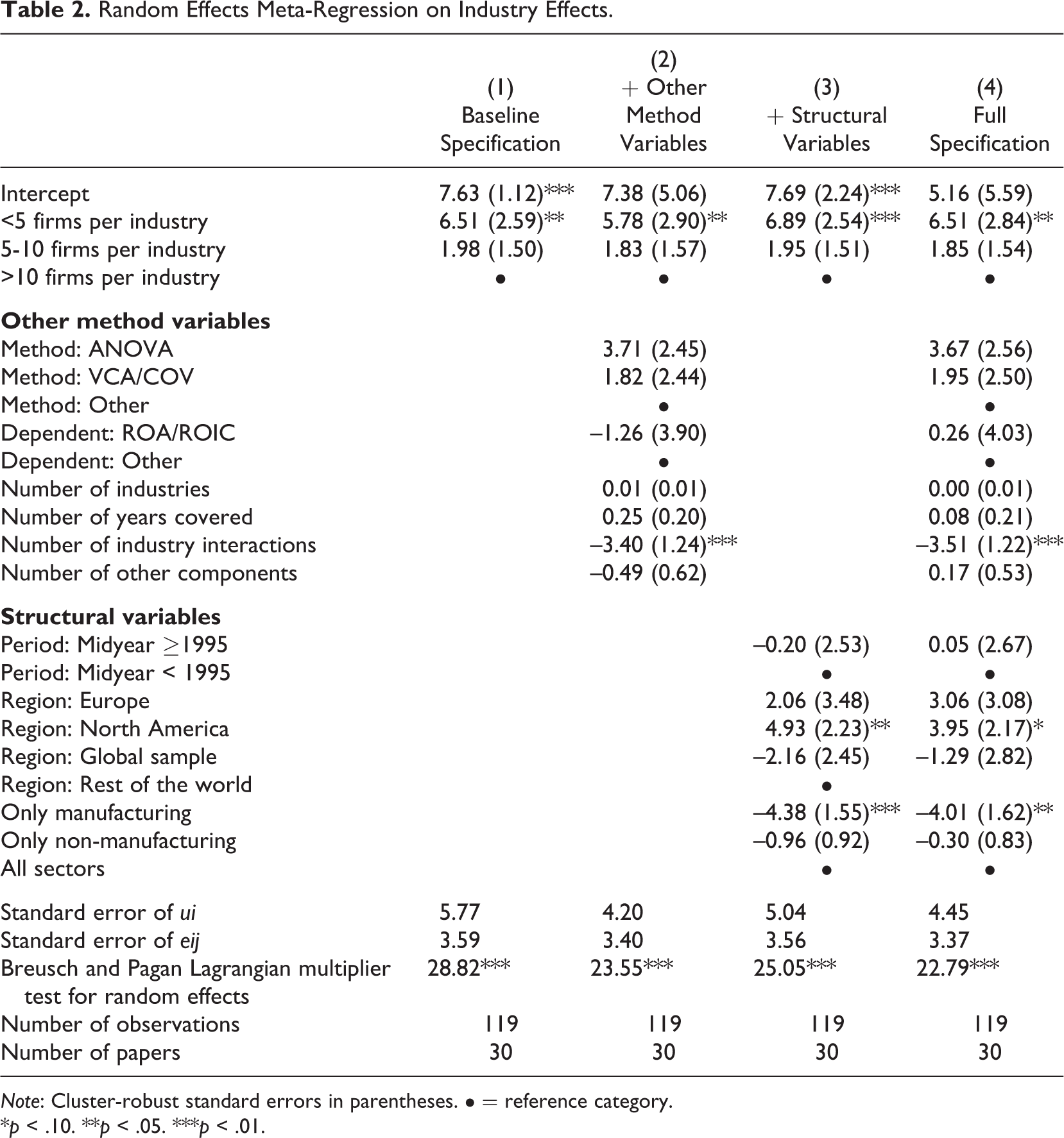
Note: Cluster-robust standard errors in parentheses. • = reference category.

*p < .10. **p < .05. ***p < .01.

The addition of other method variables and structural variables also provides meaningful insights regarding the determinants of the variation in industry effects across studies. The outcome variable (ROA/ROIC vs. other outcome variables), estimation method, period and number of years covered, number of industries, and number of other (non-industry) components included in the analysis have no significant influence on the reported industry effect. Compared with estimations that have applied methods other than ANOVA and COV, estimations that have used ANOVA report over a 4 percentage point higher industry effect, but this finding is statistically insignificant, indicating that there is much uncertainty about the true value of this parameter estimate. Conversely, the number of industry interactions, the sectoral scope of the study, and the locational scope of the study appear to matter. Consistent with our expectations, including industry interactions significantly reduces the industry effect. Compared with estimations that include no industry interaction (e.g., industry-year or industry-location components), estimations including one industry interaction report an approximately 3.5 percentage point lower industry effect. Reported industry effects are also generally higher when only considering North America than when considering a global or non-European sample or when accounting for all sectors instead of being limited to manufacturing.

Relation to Other Component Effects

In the previous paragraph, we showed that the component effects in variance decomposition studies may be strongly dependent on the number of observations per group within a given component. The meta-regression on industry effects showed that in studies in which the number of firms per industry is fewer than 5, the industry effect is considerably larger compared with studies in which the number of firms per industry is larger than 10 when controlling for other study characteristics. Although we only focused on industry effects in the previous analysis, it should be expected that the data sparseness problem is even more substantial in recent contributions that introduce detailed classifications and interactions among industry, location, and year classifications that result in a small average number of observations per group. For example, the recent study by McGahan and Victer (2010) finds a substantial home country–by-industry effect: Approximately 15% of the variance in ROA between firms can be attributed to home country industry-specific effects. Simultaneously, the study’s complete sample includes profitability information on 4,551 firms from 43 home countries and 295 industries. Although some home country–by-industry combinations are likely nonexistent, the average number of firms per home country by industry in the McGahan and Victer study is limited. This issue is likely to be even more problematic in the analyses of the subsamples that are presented (which frequently attribute an even higher share—up to almost 30%—of the variance to home country–by-industry effects).

This data sparseness problem is not restricted to the study by McGahan and Victer (2010); on the contrary, it is likely to affect other studies using a moderate number of firms, particularly those that focus on interaction effects (e.g., Chan et al., 2010; Karniouchina et al., 2013; Ma et al., 2013). Table 3 shows an overview of the 30 studies included in the meta-regression that are likely to suffer from data sparseness in one or more of the dimensions that they include because the average number of observations per group within a particular component is fewer than 10. As can be observed, half of the studies have at least one component in which the number of firms per group is less than 5; almost two-thirds of the studies have at least one component in which the number of firms per group is less than 10. Many of these studies also report very high effects on these dimensions. Whereas in the earlier studies, the industry effects were mainly based on samples with very few firms per industry, in the more recent studies, industry interaction effects particularly suffer from data sparseness problems.

Table 3.

Overview of Studies Included in Meta-Analysis With Few Observations for a Particular Component.

Study	Dimensions With Few Observations per Group	Average Reported Effect
Brito and Vasconcelos (2006)	Industry-by-country^a	12.5
Chan, Makino, and Isobe (2010)	Industry-by-region (China sample)^a	16.1
Chan, Makino, and Isobe (2010)	Industry-by-region (USA sample)^a	2.3
Chang and Hong (2002)	Industry-by-year^a	4.7
Claver, Molina, and Tari (2002)	Industry-by-year^a	3.0
Diaz Hermelo and Vassolo (2012)	Industry-by-country^b	4.0
Goldszmidt, Brito, and De Vasconcelos (2011)	Industry-by-country^a	3.2
Hawawini, Subramanian, and Verdin (2003)	Industry-by-year^a	3.6
Ketelhöhn and Quintanilla (2012)	Industry^b	14.0
Lieu and Chi (2006)	Industry^a	3.1
Lieu and Chi (2006)	Industry-by-year^a	11.2
Ma, Tong, and Fitza (2013)	Industry^a	8.0
	Industry-by-region^a	10.7
	Region-by-year^a	2.3
	Region-by-country^a	1.6
Makino, Isobe, and Chan (2004)	Industry^a	7.1
Makino, Isobe, and Chan (2004)	Country^b	5.4
Mauri and Michaels (1998)	Industry^a	6.0
McGahan (1999)	Industry^b	31.6
McGahan and Victer (2010)	Industry^b	12.0
	Industry-by-country^a	17.5
	Industry-by-year^a	8.6
	Country-by-year^b	1.7
McNamara, Aime, and Vaaler (2005)	Industry-by-year^a	4.5
Roquebert, Phillips, and Westfall (1996)	Industry^b	10.2
Roquebert, Phillips, and Westfall (1996)	Industry-by-year^a	17.9
Rumelt (1991)	Industry^a	13.0
Schmalensee (1985)	Industry^a	19.6
Tarziján and Ramirez (2010)	Industry^b	10.5

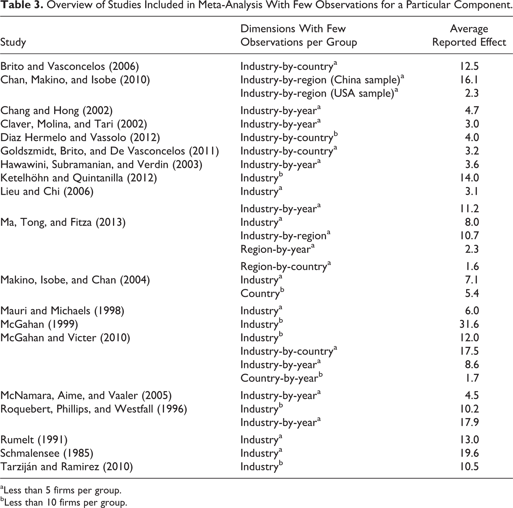
^aLess than 5 firms per group. ^bLess than 10 firms per group.

Sensitivity Analysis: Variance Decomposition Study on Firm Profitability

Critics of meta-analysis often argue that the method suffers from publication bias (see e.g. Borenstein, Hedges, Higgins, & Rothstein, 2009; Disdier & Head, 2008). The existence of a publication bias would favor those studies that find considerable industry effects in line with Schmalensee (1985) and McGahan and Porter (1997); therefore, our meta-analysis of the published literature might actually overstate the problem of data sparseness. Hence, to further examine the effect of data sparseness, we conduct a variance decomposition study using information on more than 500,000 firms in France, Italy, and Spain using a mixed hierarchical and cross-classified (multilevel) model. Firm-level data were collected from the 2012 edition of ORBIS, a commercial database provided by Bureau van Dijk. The ORBIS database provides financial and economic information on firms in almost all countries in Europe (including balance sheet and income statement items) and provides a wide range of profitability indices. ORBIS collects the most relevant database(s) of firms in each country, taking into account quality assurance, the categories of firms, and the accuracy of the information. The information is sourced from over 40 different information providers using a multitude of data sources, typically national and/or local public institutions that collect the data to fulfill legal and/or administrative requirements. Balance sheet information is collected by local chambers of commerce and disseminated in electronic format by national data providers. For this empirical exercise, we focus on firm profitability in three Mediterranean countries: France, Italy, and Spain. Overall, we have information on the firm profitability of 289,287 French firms, 125,006 Italian firms, and 209,123 Spanish firms during the 2003-2011 period. We draw several random samples (50%, 10%, 5%, and 1%) from the full data set to study the effects of data sparseness.

In addition to information on firm profitability, the database contains detailed information about the main industry sector and location of the firms. Regarding firm profitability, we focus on ROA, which is measured as the ratio of before-tax profits (or loss) to the value of the total (fixed and current) assets; ROA may be the most widely used measure of firm profitability. Only firms that provided full information for each year on certain essential financial variables (e.g., turnover, profit/loss, and total assets) were included in the sample.

Empirical Strategy

As with earlier studies by Hough (2006), Goldszmidt et al. (2011), and Van Oort, Burger, Knoben, and Raspe (2012), we use an unconditional mixed hierarchical and cross-classified (multilevel) regression model (Goldstein, 2003) to decompose the variance in firm profitability. Although previous studies have frequently used the ANOVA to decompose the variance in firm profitability, multilevel models (based on restricted maximum likelihood) tend to outperform the ANOVA (based on a methods-of-moments approach) when the number of groups for a particular component is large and the number of observations varies substantially across groups (Baltagi & Chang, 1994; Misangyi, Elms, Greckhamer, & Lepine, 2006). Because certain classifications in our model include many groupings and the number of observations varies substantially across groups within the different components, we prefer the use of a mixed hierarchical and cross-classified model to the ANOVA.⁶

Although multilevel analysis has traditionally been concerned with modeling hierarchically nested structures (e.g., firms in the same subsector that are also found in the same sector due to the nesting of the two levels), an establishment’s environment may consist of several components that have a nonhierarchical nesting structure.⁷ In other words, the components are grouped along more than one dimension or cut across hierarchies (Goldstein, 2003). In our model, we study the following components:

Year effects reflect differences in firm profitability by year.

Industry groups reflect differences in firm profitability by industry group, which are based on NACE-2 industry classifications (e.g., food manufacturing, chemicals, and financial services).

Industry sector effects reflect differences in firm profitability by industry sector, which are based on NACE-4 industry classifications (e.g., manufacture of ice cream, manufacture of perfume and toilet preparations, and pension funding).

Subregion effects reflect differences in the average firm profitability by subregion (NUTS-2 regions, e.g., Aquitaine, Lazio, or Cataluña).

Industry groups–by-subregions (e.g., financial services in Cataluña) effects reflect differences across subregions in the average firm profitability by industry group, such as through cluster effects, for example.

Industry groups–by-year effects (e.g., financial services in 2010) reflect differences across years in the average firm profitability by industry group, such as through industry life cycle effects, for example.

Firm and firm-by-year effects are reflected by total residual variation (although it may also contain other omitted effects, e.g., subregion-by-year effects).

Accordingly, we construct a three-level model (with seven components) with a random intercept i for firms and firm years at the lowest level and random intercepts for industry sectors (j1), industry groups by subregions (j2j3), industry groups by year (j2j4), industry groups (j2), subregions (j3), and years (j4) at the higher levels (see Figure 2).⁸ More formally, we estimate the following mixed hierarchical and cross-classified model for firm profitability:

Figure 2.

A three-level mixed hierarchical and cross-classified model with seven classifications.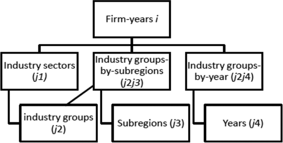

R O A_{i (j 1, j 2, j 3, j 4)} = X_{i (j 1, j 2, j 3, j 4)} β + u 0_{j 1} + u 0_{(j 2, j 3)} + u 0_{(j 2, j 4)} + u 0_{j 2} + u 0_{j 3} + u 0_{j 4} + e 0_{i (j 1, j 2, j 3, j 4)},

where firm profitability is explained by the single fixed-intercept term β, which is the average firm profitability. The six separate random terms denoted by $u 0$ are related to the intercept and mirror the remaining residual variation at the higher levels, whereas $e 0_{i (j 1, j 2, j 3, j 4)}$ reflects the firm and firm-year residual variation. This model allows us to understand how to attribute variation in accounting profitability to various components.

By taking the ratio of each variance component to the total variance, we can compute the intraclass correlation coefficient (ICC) or the variance partition coefficient. The ICC measures the extent to which accounting profitability in the same industry sector/industry group by subregion/industry group by year/industry group/subregion/year is similar relative to the firm profitability of firms in different industry sectors/industry groups by subregion/industry groups by year/industry groups/subregions/years. Alternatively, this figure may be interpreted as the proportion of the total residual variation in firm profitability that is the result of differences between the different groups within a given component.

Empirical Results

Table 4 shows the proportion of the total residual variation in firm profitability in France that is due to differences between industry sectors, industry groups by subregions, industry groups by year, industry groups, subregions, and years for different sample sizes. Focusing on the results from the 100% sample, well over 90% of the total variance in accounting profitability represents between-firm variance. Although the external environment explains a relatively small portion of the variation in firm profitability, industry and location contribute to firm performance. The between-industry sector variance and between–industry group variance are 1.84% and 1.83%, respectively; between-subregion variance accounts for less than 1% of the variance in accounting profitability. Compared with previous studies, both the industry and location effect are very modest. Turning to the interactions, we find that the result for industry group–by-subregion of 1.03% is very limited. This result is not in line with the findings of Chan et al. (2010) and Ma et al. (2013), who report an industry-by-subregion effect of between 2.3% and 16.1%. However, as indicated in the previous paragraph, the number of firms per industry–by-subregion is very small in these studies. Likewise, the industry group–by-year effect is only 0.28%. The same pattern can be observed in different empirical exercises; we arrive at similar conclusions when we reestimate our models for Italy (Table 5) and Spain (Table 6).

Table 4.

Mixed Hierarchical and Cross-Classified Model on Variation in Return on Assets (ROA) in France for different sample sizes.

	100% Sample	50% Sample	10% Sample	5% Sample	1% Sample
Year	0.62 (0.86)	0.60 (0.85)	0.55 (0.80)	0.54 (0.82)	0.73 (1.09)
Industry sectors (NACE-4)	1.84*** (0.42)	2.43*** (0.61)	2.60*** (0.82)	4.94*** (1.68)	5.13** (2.40)
Industry groups (NACE-2)	1.83 (1.24)	1.77 (1.30)	1.62 (1.58)	1.80 (2.11)	0.41 (2.06)
Subregions	0.10 (0.11)	0.10 (0.13)	0.15 (0.26)	0.01 (0.18)	0.10 (0.83)
Industry Groups × Subregion	1.03*** (0.20)	1.60*** (0.33)	4.18*** (0.93)	5.62*** (1.33)	11.44*** (3.12)
Industry Groups × Year	0.28*** (0.06)	0.27*** (0.06)	0.17** (0.07)	0.22* (0.12)	0.03 (0.17)
Number of observations	2,602,683	1,298,178	260,172	129,159	26,397
Number of firms	289,187	144,242	28,908	14,351	2,933
Number of years	9	9	9	9	9
Number of industry groups	65	65	64	64	61
Number of industry sectors	486	485	443	417	295
Number of subregions	24	22	22	22	22
Number of industry groups by subregion	1,341	1,292	1,094	974	610
Number of industry groups by year	585	585	576	576	549

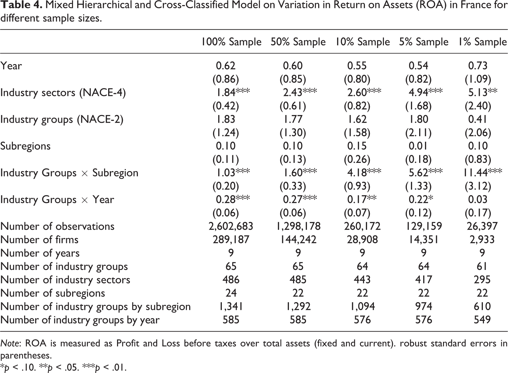
Note: ROA is measured as Profit and Loss before taxes over total assets (fixed and current). robust standard errors in parentheses.

*p < .10. **p < .05. ***p < .01.

Table 5.

Mixed Hierarchical and Cross-Classified Model on Variation in Return on Assets (ROA) in Spain for Different Sample Sizes.

	100% Sample	50% Sample	10% Sample	5% Sample	1% Sample
Year	3.85 (3.51)	3.70 (3.23)	4.04 (3.64)	4.08 (3.66)	3.59 (3.49)
Industry sectors (NACE-4)	1.39*** (0.25)	1.55*** (0.23)	3.46*** (0.71)	3.72*** (0.81)	7.52*** (2.17)
Industry groups (NACE-2)	1.63** (0.78)	1.50** (0.69)	1.39 (1.01)	1.34 (1.21)	0.89 (2.31)
Subregions	0.47 (0.55)	0.44 (0.51)	0.06 (0.12)	0.00 (0.11)	0.07 (0.36)
Industry Groups × Subregion	0.96*** (0.17)	1.58*** (0.24)	4.01*** (0.68)	5.44*** (0.99)	7.01*** (1.87)
Industry Groups × Year	1.03*** (0.14)	1.09*** (0.14)	1.05*** (0.19)	0.84*** (0.19)	0.77* (0.44)
Number of observations	1,882,107	935,793	188,244	94,536	18,414
Number of firms	209,123	103,977	20,916	10,504	2,046
Number of years	9	9	9	9	9
Number of industry groups	65	65	65	62	60
Number of industry sectors	487	481	456	426	309
Number of subregions	18	18	18	18	18
Number of industry groups by subregion	1027	995	816	723	444
Number of industry groups by year	585	585	585	558	540

Note: ROA is measured as profit and loss before taxes over total assets (fixed and current). Robust standard errors in parentheses.

*p < .10. **p < .05. ***p < .01.

Table 6.

Mixed Hierarchical and Cross-Classified Model on Variation in Return on Assets (ROA) in Italy for Different Sample Sizes.

	100% Sample	50% Sample	10% Sample	5% Sample	1% Sample
Year	1.23* (0.68)	1.28* (0.69)	1.22* (0.72)	1.23* (0.74)	1.04 (0.67)
Industry sectors (NACE-4)	2.32*** (0.25)	3.16*** (0.27)	9.62*** (1.13)	9.95*** (1.19)	19.79*** (2.87)
Industry groups (NACE-2)	1.77*** (0.53)	1.81*** (0.55)	0.40 (0.81)	—^a	—
Subregions	0.73*** (0.28)	0.58** (0.24)	0.28 (0.23)	0.24 (0.23)	0.98 (1.08)
Industry Groups × Subregion	1.70*** (0.14)	3.44*** (0.29)	9.44*** (0.88)	10.91*** (1.12)	16.84*** (2.52)
Industry Groups × Year	0.33*** (0.03)	0.30*** (0.03)	0.12*** (0.03)	0.10** (0.04)	—
Number of observations	1,125,054	563,292	112,500	56,754	10,989
Number of firms	125,006	62,588	12,500	6,306	1,221
Number of years	9	9	9	9	9
Number of industry groups	65	65	65	64	59
Number of industry sectors	623	603	530	479	309
Number of subregions	20	20	20	20	20
Number of industry groups by subregion	1,154	1,078	857	699	385
Number of industry groups by year	585	585	585	576	531

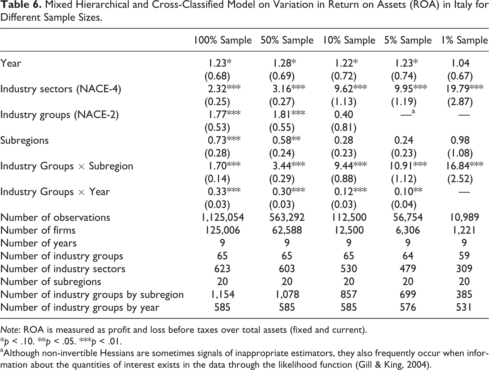
Note: ROA is measured as profit and loss before taxes over total assets (fixed and current).

*p < .10. **p < .05. ***p < .01.

^aAlthough non-invertible Hessians are sometimes signals of inappropriate estimators, they also frequently occur when information about the quantities of interest exists in the data through the likelihood function (Gill & King, 2004).

However, when we gradually reduce the complete sample to random samples of 50%, 10%, 5%, and 1%, we also see that for all three countries, the industry sector and industry groups–by-subregions (which also happen to be the components with the most groups and, therefore, the least number of observations per group) effects increase considerably. Whereas for France, the industry sector and industry groups–by-subregions effect was 1.84% (with on average 595.0 firms per industry sector) and 1.03% (with on average 185.4 firms per industry groups–by-subregion) in the full sample, respectively, these effects increase to 5.13% (with on average 9.9 firms per industry sector) and 11.44% (with on average 4.8 firms per industry groups–by-subregion) in the 1% random sample, respectively. At the same time, we see an increase in the standard errors of the variance component estimates, which indicates (not surprisingly) that when we reduce the number of observations per group within a given component, uncertainty about the true value of the estimate increases. These increases are comparable with the results found in the meta-regression.

We find similar results for Spain (Table 5). Whereas the industry sector effect was 1.39% (with on average 429.4 firms per industry sector) in the 100% sample, this effect increased to 7.52% in the 1% sample (with on average 6.6 firms per industry sector). Likewise, the industry groups–by-subregions effect in the full Spanish sample was 0.96% (with on average 203.6 firms per industry group–by-subregion) compared with 7.01% in the 1% sample (with on average 4.6 firms per industry group–by-subregion). For Italy (Table 6), the industry sector effect increased from 2.32% in the 100% sample (with on average 200.7 firms per industry sector) to 19.79% in the 1% sample (with on average 4.0 firms per industry sector), the industry groups–by-subregions effect increased from 1.70% in the 100% sample (with on average 108.3 firms per industry group–by-subregion) to 16.84% in the 1% sample (with on average 3.2 firms per industry–group-by-subregion). When comparing the findings for the different estimations across countries, we see that the differences across the different estimations are more pronounced for the Italian sample compared with the French and Spanish samples. These differences can be explained by the fact that in the 1% Italian sample, the number of firms per industry sector and industry group–by-subregion are much lower compared with the 1% French and Spanish samples.

Similar results are found when reestimating the models using different profitability measures.⁹ Accordingly, when we use a smaller data set (which also results in fewer observations per group), we are more likely to conclude that there are between–industry sector and between industry–by-subregion differences than when we utilize the complete data set. At the same time, we also observe that not all components that are subject to data sparseness show signs of inflation when moving from the 100% sample to the 1% sample. Although the number of firms per industry-year also considerably drops when moving from the 100% sample to the 1% sample, the industry-year effect remains relatively constant across the different estimations in the estimations for all three Mediterranean countries. A possible explanation for these findings is that the different group levels and particularly the interaction effects between the group levels (e.g., industry-by-region or industry-by-year effects) become indistinguishable when the average number of firms per industry greatly decreases. In such cases, shared variance can be assigned to only one of the components entered into the analysis, resulting in an underestimation of the other group-level components. However, when we take out the industry-related components and reestimate our mixed hierarchical and cross-classified model on variation in ROA in France, Spain, and Italy for different sample sizes, we still see no inflation of the industry group–by-year effect in the 1% sample.¹⁰

An alternative explanation is that the industry sector and industry group–by-subregion levels are more indistinguishable from the firm level in the 1% samples compared with the industry group–by-year levels. This would be the case if there are relatively more singletons (groups with only one observation) at the industry sector– and industry group–by-subregion levels than at the industry group–by-year level, which means that although the number of firms per group does not differ across the different components, the distribution of the number of firms per group is more skewed within the industry sector– and industry group–by-subregion levels than within the industry group–by-year level. This is indeed the case. If we look at the 1% French sample, only 7.6% of the groupings are singleton within the industry-year level, while for the industry sector– and industry group–by-subregion levels, this figure is 25.1% and 41.1%, respectively. Likewise, the number of groups with less than 5 firms per group is 21.7% for the industry-year level, while for the industry sector– and industry group–by-subregion levels, 59.6% and 73.6% of the groups have less than 5 firms, respectively.

Discussion

In this study, we have analyzed to what extent the results in variance decomposition studies on accounting profitability have been driven by data sparseness, particularly by the number of observations per group within a component. A meta-regression on industry effects showed that estimations using fewer than 5 firms per industry report an industry effect of approximately 6.5 percentage points more compared with estimations using more than 10 firms per industry when other study aspects are held constant. Because the average reported industry effect across all studies in our meta-analysis was 8.9% with an interquartile range of 4.6% to 13.6%, it can be inferred that data sparseness can result in a considerable overestimation of the industry effect. The early variance decomposition literature has left the impression that industry accounts for about 20% of the variance in firm profitability, while the “real” average industry effect is likely to be below the average of 8.9%. Similar observations can be made for more recent variance decomposition studies that have addressed the importance of industry life cycles and clusters (industries-by-location) in driving firm profitability.

Although our meta-regression focused on industry effects, a similar case can be made with regard to the assessment of location, cluster (industry-by-location) or industry life cycle (industry-by-year) effects within the context of a variance decomposition study. This claim is based on the fact that the number of observations per grouping for these components is low in several studies, while some of the estimated effects are very high. Our findings were confirmed in a sensitivity analysis where we first conducted a variance decomposition analysis on a sample of between 100,000 and 500,000 firms and subsequently reduced the complete sample to random samples of 50%, 10%, 5%, and 1%. Here, we also found a strong inflation of the effect size when the number of observations per group for a particular component falls below 5, especially when there are many groups with only one observation.

Given that our study concludes that it is likely that industry, location, regional cluster, and life cycle effects have been overestimated in at least some variance decomposition studies, our work also casts new light on conceptual issues in the strategic management literature. One of the key debates in the strategic management literature is between the resource-based view of the firm (Barney, 1991; Peteraf, 1993; Wernerfelt, 1984) and the market-based view embodied in the Structure-Conduct-Performance (SCP) model (Bain, 1968) and Porter’s five forces model (Porter, 1980).¹¹ Where the resource-based view asserts that differences in profitability can be predominantly attributed to differences in resources, capabilities, and organizational types across firms, the market-based view places more emphasis on the industry and external market organization as driver of performance differences between firms (nevertheless, it is often argued that both views complement each other). Early findings indicated that the industry effect explained approximately 20% of the performance variance. However, if the “real” industry effect is generally below the average of 8.9%, it can be questioned to what extent industry factors explain a significant proportion of the variance in accounting profitability. Similar questions can be posited with regard to the literature on firm profitability that analyzed the effects of firm diversification, industry life cycles, clusters, or institutions. Returning to the question why some firms are more profitable than others, it seems that firm effects factors are even more important than envisaged in the early literature on accounting profitability.

At the same time, it would be misguided to discard the SCP, Porter’s five forces model, or other market-based views of the firm. It is undoubtedly true that firms tend to cluster across space, some industries grow faster than other industries, and some countries outperform other countries in terms of economic growth. In addition, resources that enable a firm to outperform can be located and obtained beyond its legal boundaries (e.g., Lavie, 2006; Steinle & Schiele, 2008), albeit their availability might be geographically or sectorally constrained. Additionally, given that the boundaries of a firm can be opaque, it remains particularly unclear today the extent to which the effect of firm resources, capabilities, and organizational type on firm profitability is contingent on a firm’s external environment. In this regard, industry membership might matter less for new ventures than for established firms (Short, McKelvie, Ketchen, & Chandler, 2009) or for domestic firms compared with multinational firms (McGahan & Victer, 2010). Likewise, location might matter more for the growth of small firms than for the growth of large firms (Van Oort et al., 2012), while the effect of multinationality on firm performance might be contingent on the combination of the geographic scope of internalization and the firm’s capabilities (Kim, Hoskisson, & Lee, 2014). In terms of firm diversification, it might be important to find not only attractive industries but industries in which synergies can be created (Arend, 2009; Neffke & Henning, 2013). Hence, it is pertinent to explore the interface between firm capabilities and a firm’s external environment (see also Arend, 2009; Eriksen & Knudsen, 2003). Such firm-environment interactions have hardly been explored, and this approach would be a fruitful way forward.

Concluding Remarks

In sum, we must be careful about drawing general conclusions from previous empirical work with regard to the importance of industry, location, cluster, and life cycle effects, particularly in cases in which sample sizes and the number of observations per group are relatively low. Although one might think that the problem of data sparseness in variance decomposition studies on accounting profitability will gradually disappear thanks to the increasing availability of large amounts of data through firm databases such as ORBIS, Thomson ONE, and Compustat, at the same time attention has also shifted from analyzing industry effects to analyzing the extent to which industry effects are contingent on year and location. Such analyses typically involve more complex data structures and require larger sample sizes for variance decomposition, especially given the larger number of groups within components. In this regard, a limitation of the current study is that it predominantly highlights the problem of data sparseness in variance decomposition studies within the strategic management literature, but it does not identify minimum sample sizes or the exact conditions under which variance components results are biased. This issue would deserve more attention and should be addressed in future research.

Footnotes

Appendix A1: Descriptive Statistics for Meta-Regression

	Mean	Standard Deviation	Minimum	Maximum
Industry effect	8.92	5.91	0.2	31.6
<5 firms per Industry	0.22	0.41	0	1
5-10 firms per Industry	0.30	0.46	0	1
Other method variables
Method: ANOVA	0.29	0.45	0	1
Method: VCA/COV	0.57	0.49	0	1
Dependent: ROA/ROIC	0.91	0.29	0	1
Number of industries	183.83	204.63	5	668
Number of years covered	7.40	3.52	1	16
Number of industry interactions	0.63	0.64	0	2
Number of other components	4.14	1.49	1	9
Structural variables
Period: Midyear ≥ 1995	0.66	0.47	0	1
Region: Europe	0.13	0.33	0	1
Region: North America	0.36	0.48	0	1
Region: Global sample	0.24	0.43	0	1
Only manufacturing	0.40	0.49	0	1
Only non-manufacturing	0.08	0.27	0	1
Number of observations	119	119	119	119
Number of papers	30	30	30	30

Appendix A2: Correlation Table for Independent Variables in Meta-Regression ( N = 119)

	(1)	(2)	(3)	(4)	(5)	(6)	(7)	(8)	(9)	(10)	(11)	(12)	(13)	(14)	(15)
(1) <5 firms per Industry	1.00
(2) 5-10 firms per Industry	–0.34	1.00
(3) Method: ANOVA	0.07	–0.09	1.00
(4) Method: VCA/COV	0.09	0.09	–0.73	1.00
(5) Dependent: ROA/ROIC	–0.18	0.21	0.20	–0.16	1.00
(6) Number of industries	–0.12	0.47	0.10	–0.14	0.03	1.00
(7) Number of years covered	0.01	–0.04	0.09	0.03	–0.00	0.03	1.00
(8) Number of industry interactions	0.05	0.01	0.22	–0.02	0.23	–0.14	0.26	1.00
(9) Number of other components	0.36	–0.11	0.42	–0.24	–0.07	–0.00	0.07	0.33	1.00
(10) Period: Midyear ≥1995	–0.05	0.04	0.14	–0.11	–0.23	0.04	–0.37	0.01	0.21	1.00
(11) Region: Europe	–0.02	–0.20	0.04	–0.08	–0.05	–0.15	–0.28	0.18	–0.10	0.11	1.00
(12) Region: North America	–0.19	0.15	–0.01	–0.13	0.12	0.44	–0.03	–0.36	–0.30	–0.28	–0.29	1.00
(13) Region: Global sample	0.27	–0.20	0.07	–0.02	–0.16	–0.09	–0.10	0.12	0.51	0.40	–0.22	–0.43	1.00
(14) Only manufacturing	0.23	–0.28	0.16	–0.22	0.26	–0.20	–0.40	–0.09	0.14	0.08	0.36	0.13	0.01	1.00
(15) Only non-manufacturing	–0.15	0.08	–0.18	0.11	0.09	0.16	–0.15	–0.18	–0.05	0.20	–0.11	0.05	0.21	–0.24	1.00

Notes

Acknowledgements

We would like to thank the editors Brian K. Boyd and James M. LeBreton and three anonymous reviewers for their useful suggestions and comments on earlier versions of this paper. All errors that remain are ours.

Declaration of Conflicting Interests

The authors declared no potential conflicts of interest with respect to the research, authorship, and/or publication of this article.

Funding

The authors received no financial support for the research, authorship, and/or publication of this article.

References

Arend

R. J.

(2009). Industry and firm effects: No firm is an island. Journal of Business Research, 62 (6), 651–659.

Bain

(1968), Industrial organization. New York, NY: John Wiley and Sons.

Baltagi

Chang

Y. J.

(1994). Incomplete panels: A comparative study of alternative estimators for the unbalanced one-way error component regression model. Journal of Econometrics, 62 (2), 67–89.

Barney

(1991). Firm resources and sustained competitive advantage. Journal of Management, 17 (1), 99–120.

Bell

B. A.

Ferron

J. M.

Kromrey

J. D.

(2008). Cluster size in multilevel models: The impact of sparse data structures on point and interval estimates in two-level models. Proceedings of the Joint Statistical Meetings, Survey Research Methods Section. Retrieved from https://www.amstat.org/Sections/Srms/Proceedings/y2008/Files/300933.pdf

Bliese

P. D.

Halverson

R. R.

(1998). Group size and measures of group-level properties: An examination of eta-squared and ICC values. Journal of Management, 24 (2), 157–172.

Bonett

D. G.

(2002). Sample size requirements for estimating intraclass correlations with desired precision. Statistics in Medicine, 21 (9), 1331–1335.

Borenstein

Hedges

L. V.

Higgins

J. P. T.

Rothstein

H. R.

(2009). Introduction to meta-analysis. Chichester, UK: Wiley.

Bou

J. C.

Satorra

(2010). A multigroup structural equation approach: A demonstration by testing variation of firm profitability across EU samples. Organizational Research Methods, 13 (4), 738–766.

10.

Brito

L. A.

Vasconcelos

F. C.

(2006). How much does country matter? In Cooper

Alvarez

Carrera

Mesquita

L. F.

Vassolo

(Eds.), Entrepreneurial strategies (pp. 95–113). Oxford, UK: Blackwell.

11.

Brush

T. H.

Bromiley

(1997). What does a small corporate effect mean? A variance components simulation of corporate and business effects. Strategic Management Journal, 18, 825–835.

12.

Brush

T. H.

Bromiley

Hendrickx

(1999). The relative influence of industry and corporation on business segment performance: An alternative estimate. Strategic Management Journal, 20, 519–547.

13.

Bryk

A. S.

Raudenbush

S. W.

(1992). Hierarchical linear models: Applications and data analysis methods. Newbury Park, CA: Sage Publications.

14.

Chan

C. M.

Makino

Isobe

(2010). Does subnational region matter? Foreign affiliate performance in the United States and China. Strategic Management Journal, 31 (11), 1226–1243.

15.

Chang

S. J.

Hong

(2002). How much does the business group matter in Korea? Strategic Management Journal, 23 (3), 1226–1243.

16.

Chang

S. J.

Singh

(2000). Corporate and industry effects on business unit competitive position. Strategic Management Journal, 21 (7), 739–752.

17.

Chen

Y. M.

Lin

F. J.

(2006). Sources of superior performance: Industry versus firm effects among firms in Taiwan. European Planning Studies, 14 (6), 733–751.

18.

Clarke

(2008). When can group level clustering be ignored? Multilevel models versus single-level models with sparse data, Journal of Epidemiology and Community Health, 62 (8), 752–758.

19.

Clarke

Wheaton

(2007). Addressing data sparseness in contextual population research using cluster analysis to create synthetic neighborhoods. Sociological Methods & Research, 35 (3), 311–351.

20.

Claver

Molina

Tari

(2002). Firm and industry effects on profitability: A Spanish empirical analysis. European Management Journal, 20 (3), 321–328.

21.

De Groot

H. F. L.

Poot

Smit

M. J.

(2009). Agglomeration externalities, innovation and regional growth: theoretical reflections and meta-analysis. In Capello

Nijkamp

(Eds.), Handbook of regional growth and development theories (pp. 256–281). Cheltenham, UK: Edward Elgar.

22.

DerSimonian

Laird

(1986). Meta-analysis in clinical trials. Controlled Clinical Trials, 7 (3), 177–188.

23.

Diaz Hermelo

Vassolo

(2012). How much does country matter in emerging economies? Evidence from Latin America. International Journal of Emerging Markets, 7 (3), 263–288.

24.

Disdier

A. C.

Head

(2008). The puzzling persistence of the distance effect on bilateral trade. The Review of Economics and Statistics, 90 (1), 37–48.

25.

Eriksen

Knudsen

(2003). Industry and firm level interaction: implications for profitability. Journal of Business Research, 56 (3), 191–199.

26.

Fidalgo

E. G.

Victoria

J. V.

(2002). How much do strategic group matter? Review of Industrial Organization, 21 (1), 55–71.

27.

Gill

King

(2004). What to do when your Hessian is not invertible: Alternatives to model respecification in nonlinear estimation. Sociological Methods & Research, 33 (1), 54–87.

28.

Glass

G. V.

(1976). Primary, secondary and meta-analysis of research. Educational Researcher, 5 (10), 3–8.

29.

Goddard

Tavakoli

Wilson

(2009). Sources of variation in firm profitability and growth. Journal of Business Research, 62 (4), 495–508.

30.

Goldstein

(2003). Multilevel statistical models (3rd ed). London: Arnold.

31.

Goldszmidt

R. G. B.

Brito

L. A. L.

De Vasconcelos

F. C.

(2011). Country effect on firm performance: A multilevel approach. Journal of Business Research, 64 (3), 273–279.

32.

Hawawini

Subramanian

Verdin

(2003). Is performance driven by industry- or firm-specific factors? A new look at the evidence. Strategic Management Journal, 24 (1), 1–16.

33.

Hawawini

Subramanian

Verdin

(2004). The home country in the age of globalization: How much does it matter for firm performance? Journal of World Business, 39 (2), 121–135.

34.

Hough

J. R.

(2006). Business segment performance redux: A multilevel approach. Strategic Management Journal, 27 (1), 45–61.

35.

Hox

J. J.

(2010). Multilevel analysis: Techniques and applications. New York, NY: Routledge.

36.

Jeppesen

List

J. A.

Folmer

(2002). Environmental regulations and new plant location decision: Evidence from a meta-analysis. Journal of Regional Science, 42 (1), 19–38.

37.

Karniouchina

E. V.

Carson

S. J.

Short

J. C.

Ketchen

D. J.

(2013). Extending the firm vs. industry debate: does industry life cycle matter? Strategic Management Journal, 34 (8), 1010–1018.

38.

Kessides

(1990). Internal versus external market conditions and firm profitability: An exploratory model. The Economic Journal, 100 (402), 773–792.

39.

Ketchen

D. J.

Jr Boyd

B. K.

Bergh

D. D.

(2009). Research methodology in strategic management: past accomplishments and future challenges. Organizational Research Methods, 11 (4), 643–658.

40.

Ketelhöhn

N. W.

Quintanilla

(2012). Country effects on profitability: a multilevel approach using a sample of Central American firms. Journal of Business Research, 65 (12), 1767–1772.

41.

Kim

Hoskisson

R. E.

Lee

S-H.

(2014). Why strategic factor markets matter: “New” multinationals’ geographic diversification and firm profitability. Strategic Management Journal, 36 (4), 518–536.

42.

Klepper

(1997). Industry life cycles. Industrial and Corporate Change, 6 (1), 145–181.

43.

Kreft

De Leeuw

(1998). Introducing multilevel modeling. London: Sage Publications.

44.

Lavie

(2006). The competitive advantage of interconnected firms: An extension of the resource-based view. Academy of Management Review, 31 (3), 638–658.

45.

Lieu

Chi

(2006) How much does industry matter in Taiwan? International Journal of Business, 11 (4), 387–402.

46.

Tong

Fitza

(2013). How much does subnational region matter to foreign subsidiary performance? Evidence from Fortune Global 500 Corporations’ investment in China. Journal of International Business Studies, 44 (1), 66–87.

47.

Maas

C. J. M.

Hox

J. J.

(2004). Robustness issues in multilevel regression analysis. Statistica Neerlandica, 58 (2), 127–137.

48.

Makino

Isobe

Chan

C. M.

(2004). Does country matter? Strategic Management Journal, 25 (10), 1027–1043.

49.

Mauri

A. J.

Michaels

M. P.

(1998). Firm and industry effects within strategic management: an empirical examination. Strategic Management Journal, 19 (3), 211–219.

50.

McGahan

A. M.

(1999). The performance of US corporations: 1981-1994. The Journal of Industrial Economics, 47 (3), 373–398.

51.

McGahan

A. M.

Porter

M. E.

(1997). How much does industry matter, really? Strategic Management Journal, 18 (S1), 15–30.

52.

McGahan

A. M.

Porter

M. E.

(2002). What do we know about variance in accounting profitability? Management Science, 48 (7), 834–851.

53.

McGahan

A. M.

Victer

(2010). How much does home country matter to corporate profitability? Journal of International Business Studies, 41 (1), 142–165.

54.

McNamara

Aime

Vaaler

(2005). Is performance driven by industry- or firm-specific factors: A response to Hawawini, Subramanian and Verdin. Strategic Management Journal, 26 (11), 1075–1081.

55.

Misangyi

V. F.

Elms

Greckhamer

Lepine

J. A.

(2006). A new perspective on a fundamental debate: A multilevel approach to industry, corporate, and business unit effects. Strategic Management Journal, 27 (6), 571–590.

56.

Moineddin

Matheson

F. I.

Glazier

R. H.

(2007). A simulation study of sample size for multilevel logistic regression models. BMC Medical Research Methodology, 2007 (7), 34–43.

57.

Neffke

Henning

(2013). Skill relatedness and firm diversification. Strategic Management Journal, 34 (3), 297–316.

58.

Peteraf

M. A.

(1993). The cornerstones of competitive advantage: A resource-based view. Strategic Management Journal, 14 (3), 179–192.

59.

Peterson

M. F.

Arregle

J. L.

Martin

(2012). Multilevel models in international business research. Journal of International Business Studies, 43 (5), 451–457.

60.

Porter

M. E.

(1980). Competitive strategy. New York, NY: Free Press.

61.

Porter

(1998). Clusters and the new economics of competition. Harvard Business Review, 76 (6), 77–90.

62.

Roquebert

J. A.

Phillips

R. L.

Westfall

P. A.

(1996). Markets vs management: What “drives” profitability? Strategic Management Journal, 17 (8), 653–664.

63.

Rumelt

R. P.

(1991). How much does industry matter? Strategic Management Journal, 12 (3), 167–185.

64.

Schmalensee

(1985). Do markets differ much? American Economic Review, 75 (3), 341–351.

65.

Short

J. C.

Ketchen

D. J.

Palmer

T. B.

Hult

G. T. M.

(2007). Firm, strategic group, and industry influences on performance. Strategic Management Journal, 28 (2), 147–167.

66.

Short

J. C.

McKelvie

Ketchen

D. J.

Chandler

G. J.

(2009). Firm and industry effects on firm performance: a generalization and extension for new ventures. Strategic Entrepreneurship Journal, 3 (1), 47–65.

67.

Snijders

T. A. B.

Bosker

R. J.

(1993). Standard errors and sample sizes for two-level research. Journal of Educational Statistics, 18 (3), 237–259.

68.

Steinle

Schiele

(2008). Limits to global sourcing? Strategic consequences of dependency on international suppliers: Cluster theory, resource-based view and case studies. Journal of Purchasing & Supply Management, 14 (1), 3–14.

69.

Tarziján

Ramírez

(2011). Firm, industry and corporation effects revisited: A mixed multi-level analysis for Chilean companies. Applied Economics Letters, 18 (1), 95–100.

70.

Theall

K. P.

Scribner

Broyles

Chotalia

Simonsen

… Carlin

B. P.

(2011). Impact of small group size on neighbourhood influences in multilevel models. Journal of Epidemiology Community Health, 65 (8), 688–695.

71.

Tong

Alessandri

Reuer

Chintakananda

(2008). How much does country matter? An analysis of firms’ growth options. Journal of International Business Studies, 39 (3), 387–405.

72.

Van Oort

F. G.

Burger

M. J.

Knoben

Raspe

(2012). Multilevel approaches and the firm-agglomeration ambiguity in economic growth studies. Journal of Economic Surveys, 26 (3), 468–491.

73.

Wernerfelt

(1984). A resource-based view of the firm. Strategic Management Journal, 5 (2), 171–180.