
Abstract
Magnetoencephalography (MEG) is a method to study electrical activity in the human brain by recording the neuromagnetic field outside the head. MEG, like electroencephalography (EEG), provides an excellent, millisecond-scale time resolution, and allows the estimation of the spatial distribution of the underlying activity, in favorable cases with a localization accuracy of a few millimeters. To detect the weak neuromagnetic signals, superconducting sensors, magnetically shielded rooms, and advanced signal processing techniques are used. The analysis and interpretation of MEG data typically involves comparisons between subject groups and experimental conditions using various spatial, temporal, and spectral measures of cortical activity and connectivity. The application of MEG to cognitive neuroscience studies is illustrated with studies of spoken language processing in subjects with normal and impaired reading ability. The mapping of spatiotemporal patterns of activity within networks of cortical areas can provide useful information about the functional architecture of the brain related to sensory and cognitive processing, including language, memory, attention, and perception.
In magnetoencephalography (MEG), the electrical activity of the human brain is studied noninvasively by recording magnetic fields generated by neural events (Cohen, 1972; Hamalainen, Hari, Ilmoniemi, Knuutila, & Lounasmaa, 1993; Hansen, Kringelbach, & Salmelin, 2010; Supek & Aine, 2014). MEG and electroencephalography (EEG) signals are closely related, both originating from neural currents in the brain. Whereas EEG electrodes record the scalp potential, MEG sensors measure the magnetic field outside the head. MEG and EEG signals provide a view of brain activity in the millisecond time scale. This is different from the hemodynamic measures of brain activity, such as the blood oxygenation level dependent (BOLD) contrast measured with functional magnetic resonance imaging (fMRI), which peaks seconds after the neural activity occurred. The high time resolution of MEG and EEG allows the identification of sequences of activations among multiple brain regions associated with the performance of cognitive tasks. Furthermore, the time resolution enables the examination of rhythmic, oscillatory neural activity in different frequency bands, which are believed to play an important role in brain function (Buzsaki, 2006).
By measuring the spatial distribution of the magnetic field outside the head, the locations of the neural sources of the MEG signals can be estimated. The spatial resolution of MEG depends on the characteristics of the underlying activity. A single region of focal activity can be accurately localized within a few millimeters (Cohen et al., 1990; Mosher, Spencer, Leahy, & Lewis, 1993), but localizing widespread distributed patterns of simultaneous activity in multiple areas can be challenging, as we will discuss below.
MEG is used clinically in the presurgical evaluation of patients with epilepsy (Bagic, Knowlton, Rose, & Ebersole, 2011; Burgess et al., 2011; Shibasaki, Ikeda, & Nagamine, 2007; Stufflebeam, Tanaka, & Ahlfors, 2009). Research applications of MEG include studies aimed at characterizing brain activity related to various sensory, motor, and cognitive processes, including attention, memory, and language, in normal development, as well the changes in these processes with age (see, e.g., Hari & Salmelin, 2012). In the field of neuroeconomics, MEG has been used to reveal neural processes associated with decision making and choice bias (Braeutigam, Rose, Swithenby, & Ambler, 2004; Hedgcock, Crowe, Leuthold, & Georgopoulos, 2010). MEG also serves as a powerful tool used to study atypical brain activation patterns in patients with neurological or psychiatric disorders, such as Alzheimer’s disease, schizophrenia, obsessive-compulsive disorder, autism spectrum disorder, or dyslexia (Ciesielski & Stephen, 2014; Maestu et al., 2015; Makela, 2010; Mody, 2014; Wilson, Heinrichs-Graham, Proskovec, & McDermott, 2016).
In this article, we describe basic principles and techniques of MEG data acquisition, analysis, and interpretation. The goal is to help those in the field of organizational research studies and related areas to understand the MEG method, its possibilities and limitations for addressing questions in their own area of research (see also Braeutigam, 2014; Senior, Lee, & Braeutigam, 2015), as well as to help guide their understanding of findings reported in existing MEG literature. We illustrate the use of MEG in cognitive neuroscience research with two previously published studies of spoken language processing.
Recording and Analysis of Neuromagnetic Fields
MEG Data Acquisition
The magnetic fields generated by human brain activity are weak, of the order of only about one billionth of the earth’s magnetic field (Hamalainen et al., 1993). In MEG, these fields are recorded using superconducting quantum interference device (SQUID) detectors. David Cohen made the first SQUID recording of human MEG signal using a single sensor instrument (Cohen, 1972). Modern commercially available whole-head MEG systems have several hundred sensors, arranged in a helmet-shaped array (Figure 1). The sensors are housed inside a thermal vessel called Dewar filled with liquid helium. Data may be collected with the subject in sitting or supine position, the head inside the helmet as close as possible to the sensors.

MEG instrumentation. (a) A whole-head MEG system (manufactured by Elekta-Neuromag, Helsinki, Finland) with a subject observing visual stimuli projected on a screen. (b) The door of a magnetically shielded room constructed with layers of aluminum and special high magnetic permeability material (Imedco, Haegendorf, Switzerland). (c) The layout of the sensor array of the 306-channel MEG system with 102 triple-sensor units, depicted with a cortical surface reconstructed from structural magnetic resonance images (MRI).
An example of averaged event-related MEG and EEG signals is shown in Figure 2a. The topographic maps depict the data at one time instant (in this case 100 ms after the onset of an auditory stimulus), whereas the waveforms depict the time course of the MEG signal at one SQUID sensor and the EEG signal at one scalp electrode. Figure 2b shows the corresponding data transformed to the source space: The estimated spatial distribution of the activity at the 100-ms latency is shown on the cortical surface reconstructed from the subject’s MRI, together with the time course of estimated activity in the primary auditory cortex.
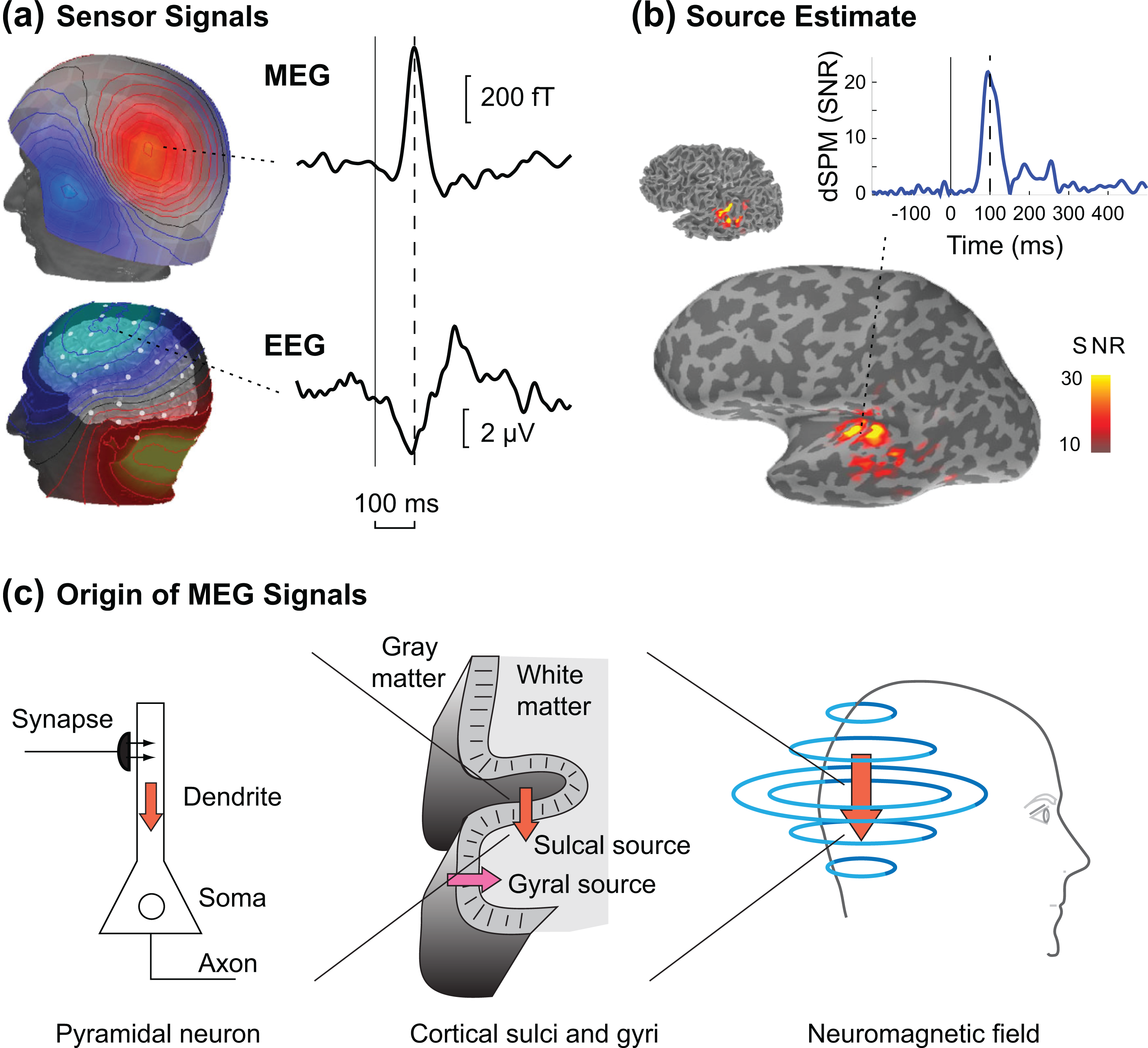
MEG signals and source estimates. (a) Topographic maps of auditory evoked magnetic fields (MEG) and electric scalp potentials (EEG) showing the spatial patterns of the recorded signals at one time point (100 ms after the onset of the sound stimulus). The MEG map depicts the magnetic field component approximately radial to the surface of the head, illustrating a typical “dipolar” pattern with peaks of opposite sign on both sides of a focal source in the auditory cortex. The waveforms show the time course of the signal recorded by one MEG and one EEG sensor, respectively. (b) A distributed source estimate (the dynamic statistical parametric map, dSPM, as a measure of the signal-to-noise ratio, SNR) for the auditory evoked response at 100 ms latency is shown on the cerebral cortex reconstructed from MRI. The cortical surface was inflated (bottom) to better visualize activity within sulci. The waveform shows the estimated time course at one source location in the left hemisphere auditory cortex. (c) Physiological origin of MEG signals. The neuromagnetic fields recorded by MEG, like the scalp potentials recorded by EEG, are mainly generated by postsynaptic dendritic currents in cortical pyramidal cells (left). The primary currents, represented here by the arrows, can be assumed to be oriented perpendicular to the cortical surface (middle). Thus, the source currents on gyral crowns and sulcal walls are typically at a right angle to each other. MEG is sensitive only to sources that are tangential, i.e., oriented perpendicular to the skull surface, but insensitive to radial sources (right). In this example, the downward pointing arrow represents a tangential, MEG-visible source on a sulcal wall in the occipital cortex, whereas the rightward pointing arrow is a radial source that is poorly visible to MEG. (a) and (b) adapted from Ahlfors and Hamalainen (2012).
MEG data can be affected by many types of unwanted artifact signals (Gross et al., 2013). Environmental magnetic noise, such as that due to machinery, elevators, or nearby street traffic, can be effectively reduced by magnetically shielded rooms and differential (gradiometric) sensors (Cohen & Halgren, 2009; Parkkonen, 2010). Frequency domain filtering is used to remove power line interference (50 or 60 Hz). For artifacts caused by the subject, such as magnetic fields generated by blinks, eye movements, and cardiac activity, shielding is impractical and one has to rely on signal processing methods. Noise from many types of sources can be efficiently suppressed by spatial filtering techniques, such as the signal space projection (SSP; Ramirez, Kopell, Butson, Hiner, & Baillet, 2011; Tesche et al., 1995; Uusitalo & Ilmoniemi, 1997), signal space separation (SSS; Taulu, Kajola, & Simola, 2004), principal component analysis (PCA), and independent component analysis (ICA; Iversen & Makeig, 2014; Luckhoo et al., 2012; Ramkumar, Parkkonen, Hari, & Hyvarinen, 2012; Tang, Pearlmutter, Malaszenko, Phung, & Reeb, 2002; Vigario, Sarela, Jousmaki, Hamalainen, & Oja, 2000). In the SSP approach, spatial patterns of the magnetic field associated with the artifacts are identified and subsequently removed using orthogonal projection methods in the multidimensional signal space. The SSS method decomposes the multichannel MEG data based on physical properties of magnetic fields, effectively separating parts of the signals that originate from inside versus outside the head. In PCA and ICA, spatiotemporal decompositions of the data are constructed, and the artifact related components are identified and removed. For the detection and removal of physiological artifacts in the MEG data, such as those related to eye movement and blinks, cardiac cycle, and muscle activity, it is helpful to record electrooculogram (EOG), electrocardiogram (ECG), and electromyogram (EMG) data simultaneously with MEG. To minimize high-frequency artifacts related to muscle activity, it is important to ensure that the subject is relaxed during the MEG session. Demagnetizing the subject with a hand-held degausser before the MEG session often helps to substantially reduce artifacts from dental work.
Forward Modeling: Generation of the Neuromagnetic Fields
The neural sources of MEG and EEG signals can be represented as primary currents, originating mainly from postsynaptic currents in the dendrites of cortical pyramidal cells (Figure 2c; Lopes da Silva, 2010; Tripp, 1983). The summed effect of postsynaptic currents within a few cubic millimeters of cortical gray matter can be approximated by a current dipole. For symmetry reasons, the primary currents can be assumed to be oriented perpendicular to the local surface of the cortex, because contributions from laterally oriented dendrites cancel out macroscopically. Computational neural models of cell membrane potentials and dendritic currents have helped provide insights into the generation of MEG signals (Ahlfors et al., 2015; Ahlfors & Wreh, 2015; Jones, Pritchett, Stufflebeam, Hamalainen, & Moore, 2007; Murakami & Okada, 2006).
The relationship between neural activity, the MEG signals, and the MEG source estimates is illustrated in Figure 3. Calculating the neuromagnetic field from a given pattern of neural activity is called the forward problem, whereas estimating the source pattern on the basis of the measured MEG signals is called the inverse problem. Source estimates may be validated by comparing them to the patterns of neural activity determined with other methods, such as intracranial recordings (Dalal et al., 2009; Halgren, Marinkovic, & Chauvel, 1998; Santiuste et al., 2008).
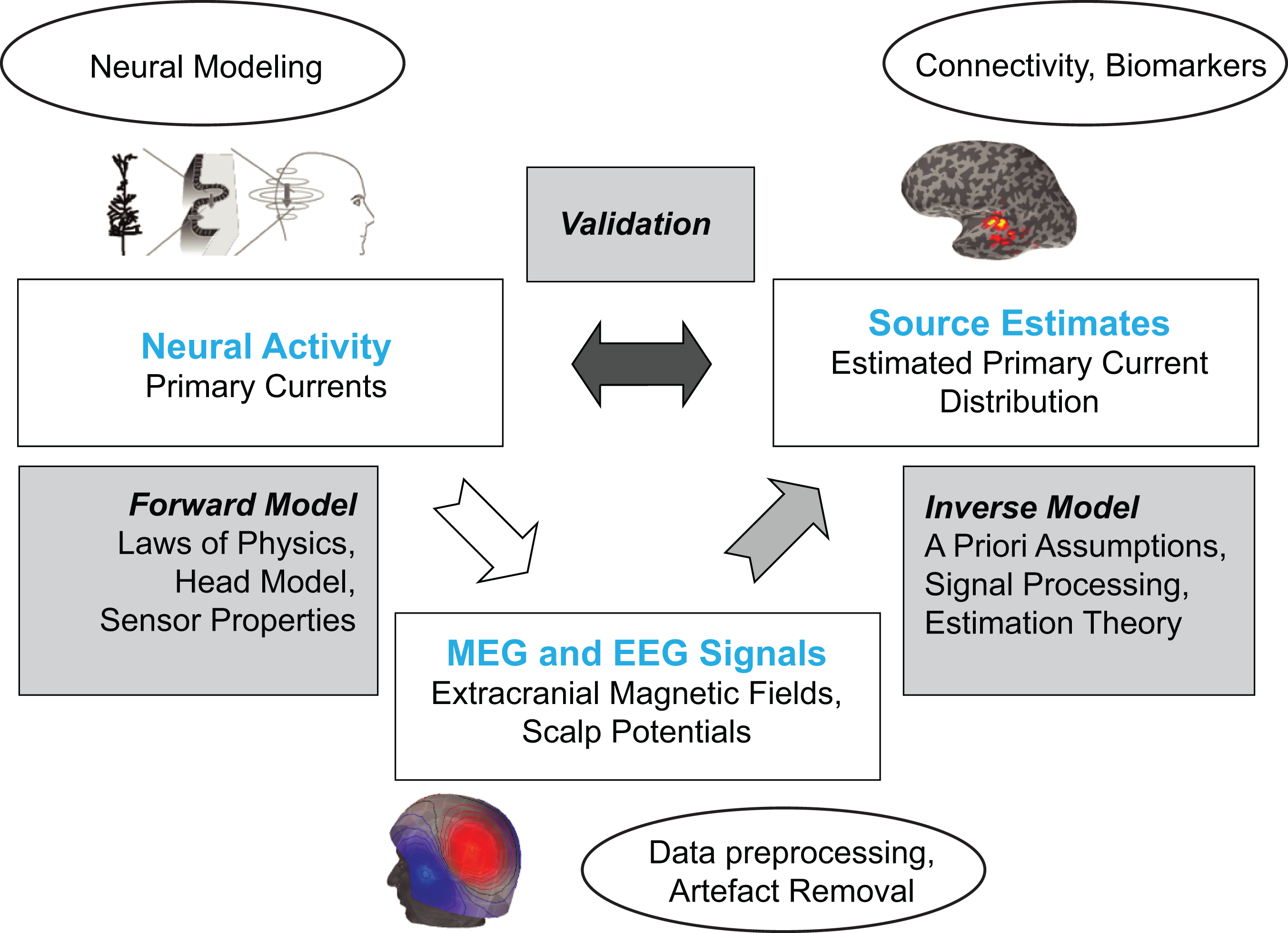
Concepts related to MEG (and EEG) signal generation and analysis. Forward and inverse models are used to estimate the spatiotemporal patterns of neural activity underlying the recorded signals. The source estimates lend themselves to modeling network dynamics and connectivity.
The MEG forward model describes what the signals in the MEG sensor array would be for a given distribution of primary currents (de Munck, Wolters, & Clerc, 2012; Hamalainen & Sarvas, 1989; Mosher, Leahy, & Lewis, 1999). The forward model incorporates the laws of electromagnetism, the shape and electrical conductivity properties of the head, and the properties of the MEG sensors. A simple spherical head approximation often works quite well for the MEG forward model, and is useful when anatomical information from structural MRI is not available. Commonly, however, a Boundary Element Model (BEM), comprising the skull and scalp surfaces derived from MRI is used (Hamalainen & Sarvas, 1989; Oostendorp & van Oosterom, 1989). With Finite Element Models (FEM), more detailed information about tissue properties can be included, such as anisotropic (direction-dependent) conductivities within the white matter, or complex shapes of regions containing cerebrospinal fluid (Haueisen et al., 2002; Wolters et al., 2006). For a comprehensive review of MEG and EEG forward modeling, see de Munck et al. (2012).
A characteristic property of MEG is that the neuromagnetic fields outside the head are almost exclusively generated by primary currents oriented tangentially with respect to the inner surface of the skull, whereas MEG is insensitive to radially oriented primary currents (Ahlfors, Han, Belliveau, & Hamalainen, 2010; Cohen & Cuffin, 1983; Grynszpan & Geselowitz, 1973). The orientation sensitivity is one of the most important differences between MEG and EEG (see the “MEG and Multimodal Brain Imaging” section below). The selective sensitivity of MEG to tangential versus radial sources is typically manifested in differential local sensitivity to sulcal versus gyral regions of the cerebral cortex. For example, in Figure 2c the gyral source is radially oriented and thus not visible to MEG. The amplitude of the MEG signal depends also strongly on the depth of the source. In general, MEG is most sensitive to superficial sources in the cerebral cortex (Cohen & Cuffin, 1983; Hillebrand & Barnes, 2002); however, there are a growing number of MEG studies describing recordings of subcortical activity (Attal & Schwartz, 2013; Garolera et al., 2007; L. Liu, Ioannides, & Streit, 1999; Ribary et al., 1991; Roux, Wibral, Singer, Aru, & Uhlhaas, 2013; Tesche, 1996).
Inverse Modeling: Estimating the Neural Sources of the MEG Signals
The MEG inverse problem refers to the process of estimating the distribution of primary currents in the brain, given the MEG signals measured outside the head (see, e.g., Ahlfors & Hamalainen, 2012; Baillet, Mosher, & Leahy, 2001). The inverse model maps the “sensor space” signals to the “source space.” The time series data measured by the MEG sensor array are transformed to a set of estimated source activation time series for a number of locations in the brain. The inverse problem is often the most challenging part of MEG data analysis and interpretation. The several hundred data values recorded outside the head at each time instant cannot, obviously, fully resolve activity among the billions of neurons in the brain. The solutions to the bioelectromagnetic inverse problem are nonunique in the sense that different source patterns in the brain can generate identical MEG (or EEG) signals. To choose meaningful inverse solutions among all the possible ones, a priori assumptions about the expected spatial distributions of activity are essential (Kaipio & Somersalo, 2004). Notably, different a priori assumptions lead to different source estimates, even for the same experimentally recorded data (Fuchs, Wagner, Kohler, & Wischmann, 1999; Shiraishi et al., 2011).
Common source estimation approaches include equivalent current dipole (ECD) models and distributed source models. In the ECD approach, the sources of the MEG signals are assumed to consist of a small number (typically fewer than 10) of focal activations, each modeled with an ECD (Hamalainen et al., 1993; Mosher et al., 1993; Scherg & Von Cramon, 1986). The locations of the ECDs can be determined using nonlinear optimization algorithms (Hamalainen et al., 1993; Huang et al., 1998) or subspace scanning techniques such as the MUSIC method (Mosher, Lewis, & Leahy, 1992). In the spatiotemporal ECD model (Scherg & Von Cramon, 1986), the locations are assumed fixed over a time window, with varying dipole moments. ECDs are well suited for representing local activations within a few square centimeters of cortical surface (de Munck, van Dijk, & Spekreijse, 1988).
When the MEG signals are generated by widespread activity, distributed source models may be more appropriate than the ECD models (Hamalainen & Ilmoniemi, 1994). In distributed source models, the primary currents are represented with a large number (typically thousands) of current dipoles at fixed locations in the brain, often spread over the cortical surface a few millimeters apart from each other (Dale & Sereno, 1993). Commonly used distributed source estimates, based on different assumptions about the amplitude distribution of the source elements, include the minimum L2-norm estimate (MNE), the minimum L1-norm estimate, the dynamical statistical parametric mapping (dSPM), and the low resolution electrical tomography (LORETA). The MNE (Hamalainen & Ilmoniemi, 1994) assumes minimum power for the estimated source current distribution, and typically provides smooth widespread solutions. In MNE, the maximum amplitude is located in superficial parts of the brain, unless depth-weighting is applied (Fuchs et al., 1999; F. H. Lin et al., 2006). The LORETA method (Pascual-Marqui, Michel, & Lehmann, 1994) assumes spatial smoothness by explicitly preferring similar amplitudes between neighboring locations. The dSPM (Dale et al., 2000) and the related sLORETA method (Pascual-Marqui, 2002; Wagner, Fuchs, & Kastner, 2004) provide estimates for the signal-to-noise ratio of the source currents. The minimum L1-norm solutions (Matsuura & Okabe, 1997; Uutela, Hamalainen, & Somersalo, 1999), also known as the minimum-current estimate (MCE), provide spatially sparse source estimates. A potential inconvenience with the sparse methods is that the time courses for given brain regions are not temporally smooth, even when the original recorded MEG data are smooth; to address this issue, mixed-norm methods have been proposed (Ding & He, 2008; Gramfort, Strohmeier, Haueisen, Hamalainen, & Kowalski, 2013; Ou, Hamalainen, & Golland, 2009).
Another widely used source estimation approach is the beamformer method, which maps the potential source locations with a spatial filter (Hillebrand, Singh, Holliday, Furlong, & Barnes, 2005; Sekihara & Nagarajan, 2008; Van Veen, van Drongelen, Yuchtman, & Suzuki, 1997; Vrba & Robinson, 2001). In adaptive beamforming, the spatial filter is based on the data covariance matrix, whereas nonadaptive beamformers can be constructed using a priori assumptions about the expected locations of the sources of interest.
Paradigmatic, Population, and Practical Constraints in MEG Studies
As with any neuroimaging study, the importance of careful experimental design and piloting should not be underestimated when using MEG in research. Eye movements, eye blinks, time intervals between stimuli, passive versus response-dependent activation, needs of special clinical populations, head size, and distance from the sensors in children are among the crucial factors for a successful MEG study (Gross et al., 2013). The MEG environment typically allows a flexible set of experimental designs, including stimulus delivery in different sensory modalities (visual, auditory, somatosensory) and recording of motor response (buttons, joystick). Besides task-related activity, the recording of spontaneous, resting state activity is common.
The instrumentation, however, does pose some limitations on the types of studies that can be conducted using MEG. The sensors are in a fixed array inside a cryogenic Dewar vessel (see Figure 1). Therefore, the subject cannot move freely (which, in principle, is possible with EEG). In contrast to many MRI systems, however, the subjects have an open view while positioned in the MEG helmet and rarely feel claustrophobic. Many MEG systems have the option of recording with the subject in either sitting or supine position, which helps the subject to stay alert during cognitive tasks (sitting position) or fall asleep in sleep studies (supine). Some populations, such as, children with attention-deficit/hyperactivity disorder or autism spectrum disorder, may require special coaching for the MEG recording session (Mody & Christodoulou, 2013). Of significance to these populations is the subject preparation time which is greatly reduced in MEG compared with EEG as there is no application of electrodes (though newer EEG systems offer dry or quick electrode application alternatives). For overall signal quality, it is important that the subject stays still during the recording. It is also essential that the subject’s head stays as close to the MEG sensor array as possible, because the magnitude of the neuromagnetic signals decreases rapidly when the distance from the brain increases. For subjects with a small head, it may be advantageous to position the head such that those brain areas that are of most interest in a particular study (e.g., left vs. right hemisphere, or occipital vs. frontal regions) will be closest to the sensor array (Marinkovic, Cox, Reid, & Halgren, 2004). MEG systems designed specifically for pediatric studies have also been introduced (Okada et al., 2006).
Recently, there have been efforts to obtain MEG data related to social interactions, opening up exciting new options for the use of MEG (Hari, Himberg, Nummenmaa, Hamalainen, & Parkkonen, 2013). In principle, one could have in the future two MEG systems in the shielded room, with the subjects interacting with each other. However, a more readily available solution is to record MEG (and EEG) in one subject and EEG in another subject simultaneously inside the MEG room. Importantly, if another person is inside the shielded room, as may also be necessary with pediatric and certain clinical populations to ensure that the participant stays still and follows instructions, this person should have all magnetic materials removed and should not move during the MEG recording to minimize signal artifacts in the data.
There are significant expenses, comparable to those for an MRI scanner, related to the initial cost of the MEG instrument and the magnetically shielded room. Running costs include the supply of liquid helium, which can be substantially reduced by systems allowing helium recycling, and support for an operating technician in a laboratory or hospital environment. The marginal cost of running a subject is relatively low. The subject preparation can be done in about 15 minutes, which is typically much shorter than that required for a high-density EEG recording. The duration of the MEG data recording is usually somewhere between 10 minutes and 2 hours, depending on the experimental paradigm. For task-related activity, trials typically need to be repeated several tens of times to achieve adequate signal-to-noise ratio by data averaging.
MEG and Multimodal Brain Imaging
Over the past two decades, multimodal imaging has highlighted the numerous advantages of integrating different types of neuroimaging data (He & Liu, 2008; Poline, Garnero, & Lahaue, 2010). In this section, we discuss the use of MEG in combination with EEG, structural MRI, and functional MRI .
MEG and EEG are commonly recorded simultaneously, with integrated data acquisition systems and nonmagnetic EEG electrode caps. Although the physiological origin of MEG and EEG signals is the same, described as the primary current distribution in the brain, MEG and EEG have complementary spatial sensitivity profiles (Cohen & Cuffin, 1983). Both MEG and EEG are most sensitive to superficial cortical activity; however, EEG has better sensitivity than MEG to deep sources, whereas MEG provides a better spatial resolution of superficial sources (de Jongh, de Munck, Goncalves, & Ossenblok, 2005; Goldenholz et al., 2009; Hunold, Funke, Eichardt, Stenroos, & Haueisen, 2016). Furthermore, MEG is sensitive only to tangentially oriented source currents, often corresponding to activity in sulcal walls (see Figure 2c), whereas EEG is sensitive to both tangential and radial source currents (Ahlfors et al., 2010; Cohen & Cuffin, 1983; Haueisen, Ramon, Czapski, & Eiselt, 1995). The selective sensitivity of MEG to only some source components can actually be considered a benefit of MEG, because it simplifies the interpretation of the data, and reduces contributions from background brain activity unrelated to the task, sometimes referred to as “brain noise.” Combining MEG and EEG data can improve the source localization accuracy (Babiloni et al., 2001; Mosher et al., 1993; Sharon, Hamalainen, Tootell, Halgren, & Belliveau, 2007). In general, the same source estimation techniques are applicable for both EEG and MEG (Michel & Murray, 2012). To some extent, the analysis of combined MEG and EEG has been difficult in practice due to a lack of a clear framework for preprocessing and merging of these data using well-established toolboxes. However, several powerful analysis software packages are presently available (Baillet, Friston, & Oostenveld, 2011). Combined MEG and EEG recordings also reduce the chances of missing some activity due to differences in the sensitivity and signal-to-noise ratio (de Jongh et al., 2005; Goldenholz et al., 2009). For example, interictal epileptic spikes may be evident only in MEG or only in EEG (Knake et al., 2006; Y. Y. Lin et al., 2003; Ossenblok, de Munck, Colon, Drolsbach, & Boon, 2007; Ramantani et al., 2006; Rodin, Funke, Berg, & Matsuo, 2004). It should be noted, however, that due to, for example, magnetic or excessive movement artifacts, not all subjects are compatible for MEG.
Simultaneous recording of MEG and MRI is not feasible at present, although new developments in special hardware may make it possible to record MRI using the MEG sensors (Vesanen et al., 2013; Zotev et al., 2008). However, including separately obtained structural MRI data is common in the analysis and interpretation of MEG data. Anatomical information from MRI is used to construct the BEM or FEM head model for the forward problem, to constrain the locations of MEG sources on the cortical surface in the inverse problem, and to visualize the estimated source activity with respect to anatomy. To coregister the MEG and structural MRI data, it is necessary to know the locations of the MEG sensors with respect to anatomical landmarks. For this purpose, 3 to 5 small head position indicator (HPI) coils are attached to the subject’s head during MEG data acquisition. These coils can be localized in relation to the MEG sensor array on the basis of the magnetic signals they generate in the MEG sensors. A 3D digitizer is used to determine the locations of the HPI coils with respect to anatomical landmarks, such as the nasion and preauricular points, identifiable in structural MRI data. The HPI information can also be used to compensate for head movements that occurred during the recording session (Taulu & Simola, 2006; Uutela, Taulu, & Hamalainen, 2001; Wehner, Hamalainen, Mody, & Ahlfors, 2008).
The complementary spatial and temporal sensitivity properties of hemodynamic (fMRI) and electrophysiological (MEG, EEG) imaging modalities suggest that combining these different types of data can provide more information about brain function than any single modality alone. In particular, the millisecond time resolution of MEG and EEG complement the good spatial resolution of fMRI. The main approaches to combining fMRI with MEG and EEG data are converging evidence, direct data fusion, and computational neural modeling (Horwitz & Poeppel, 2002). Converging evidence from the comparison of separately obtained results can be helpful for assessing the reliability of the observed activation patterns; for example, fMRI can be used to confirm locations of active regions seen in MEG source estimates. In direct data fusion, data from different modalities are combined in mathematical analyses. One example is the use of fMRI to guide the MEG source estimation. In particular, fMRI can suggest likely source configurations among all the possible ones that could have generated the recorded MEG data (Ahlfors et al., 1999; Ahlfors & Simpson, 2004; A. K. Liu, Belliveau, & Dale, 1998). Direct data fusion can be problematic because the exact nature of the physiological origin of fMRI and MEG/EEG signals is not known; however, there is experimental evidence that the BOLD contrast seen by fMRI and the postsynaptic currents seen by MEG and EEG are closely correlated (Logothetis, Pauls, Augath, Trinath, & Oeltermann, 2001). In fMRI-guided MEG/EEG source estimation, one has to consider the effects caused by possible differences in the spatial distribution of activity seen by the different modalities (for further discussion, see Ahlfors, 2014; Ahlfors & Simpson, 2004; A. K. Liu et al., 1998). In the future, developments in computational modeling of neural activity may enable the merging of the different types of imaging signals into a common neurophysiological model (Babajani, Nekooei, & Soltanian-Zadeh, 2005; Bojak, Oostendorp, Reid, & Kotter, 2011; Horwitz & Poeppel, 2002; Plis, Calhoun, Weisend, Eichele, & Lane, 2010; Valdes-Sosa et al., 2009).
MEG Measures and Interpretation
MEG data lend themselves to a number of quantitative metrics. From the time series data, various measures can be extracted, such as peak latencies and amplitudes, spectral peaks, time-frequency components, and connectivity properties. The time series can be taken either directly from the sensor data recorded by individual MEG sensors, or from the source estimates obtained by inverse modeling. The interpretation of the sensor data is limited because there is uncertainty about where in the brain the activity originates, and because the sensor signals contain a mixture of contributions from multiple brain sources. Transforming the sensor data into source estimates can often provide a physiologically meaningful way to unmix the signals and help to interpret the measures in terms of brain regions.
Statistical analyses are performed to identify differences in the derived measures between experimental conditions and/or subject groups (Pantazis et al., 2009). In practice, it is usually necessary to reduce the amount of data to be submitted to the statistical analysis to alleviate problems associated with multiple comparisons. One approach for handling the multiple comparison problem is to use nonparametric permutation tests in which data are clustered on the basis of spatial, temporal, and/or spectral adjacency (Maris & Oostenveld, 2007). Another way is to select regions of interest (ROIs). ROIs in space, time, and/or frequency domains can be identified using the “omnibus” data, in which all subjects and experimental conditions are combined. Combining all data for the ROI selection is important to avoid preselection bias in the statistical comparisons between groups or conditions. The ROI selection can also be guided by data from other imaging modalities, such as, time windows of established event-related potential (ERP) components in EEG, or spatial patterns of activity in fMRI.
Time-frequency analyses can reveal the evolution of oscillatory activity within different spectral bands over time. Time-frequency representations are usually computed with wavelet or multitaper methods (Mitra & Pesaran, 1999; Tallon-Baudry, Bertrand, Delpuech, & Permier, 1997). The most commonly used frequency bands are the classical EEG bands: theta (4-8 Hz), alpha (9-14 Hz), beta (15-30 Hz), and gamma (>30 Hz; Niedermeyer & Lopes da Silva, 2005). The time-frequency transformation is often also the starting point for connectivity analyses, helping to differentiate between local and long-distance connectivity (Brookes et al., 2011; de Pasquale et al., 2012; Hipp, Hawellek, Corbetta, Siegel, & Engel, 2012; Palva & Palva, 2012). Functional connectivity measures, which indicate statistical interdependency in the activities in different brain regions, include imaginary coherence and phase locking (Gross et al., 2001; Lachaux, Rodriguez, Martinerie, & Varela, 1999; Nolte et al., 2004). Directional influence between areas can be evaluated with effective connectivity techniques, such as Granger causality, transfer entropy, and dynamic causal modeling (Friston, Moran, & Seth, 2013; Gow, Segawa, Ahlfors, & Lin, 2008; Greenblatt, Pflieger, & Ossadtchi, 2012; F. H. Lin et al., 2004; Wibral et al., 2011). MEG data also lend themselves to cross-frequency analyses, providing another approach to examine local connectivity by measuring phase-amplitude coupling between different frequency bands (Canolty & Knight, 2010).
Examples of MEG Studies
Among the many applications of MEG to cognitive neuroscience, our understanding of language processing and its neurocognitive underpinnings is one area that has benefited from advances in brain imaging. Taking advantage of the temporal resolution of MEG, researchers are getting closer to teasing apart component processes (e.g., phonology, semantics, and syntax) intertwined in the speech signal toward development of neurocognitive models of language (Garagnani, Shtyrov, & Pulvermuller, 2009; Gow & Nied, 2014; Lau & Nguyen, 2015; Overath, McDermott, Zarate, & Poeppel, 2015). To illustrate the use of MEG and different analysis methods to study patterns of cortical activity in the human brain, we describe two studies of phonological processing in auditory word discrimination (Wehner, Ahlfors, & Mody, 2007) and in sentence comprehension (Han, Mody, & Ahlfors, 2012). These studies highlight the interactions between lower level perceptual processes and top-down semantic influences in speech perception.
Reduced Left Temporal Activation in Poor Readers During Phonologically Demanding Speech Perception
Children with reading disabilities appear to have deficient phonological (i.e., speech sound) representations. In an MEG study, Wehner et al. (2007) used a speech perception task to compare the brain activation patterns between normal and impaired readers to better understand the phonological basis in reading disability. Two groups of 7- to 13-year-old children, 15 good readers and 15 poor readers, performed an auditory oddball task while MEG was recorded. In this task, occasional deviant stimuli (the word “bat,” “cat,” or “rat”) were presented among a repeated standard stimulus (“pat”; Figure 4a). The subjects were instructed to press a button as soon as they heard any of the deviant stimuli. Averaged event-related responses for one subject in an MEG sensor are shown in Figure 4b. The waveforms show the difference in the responses to deviant and standard stimuli. Prominent responses are seen in the latency range of the phonological mismatch negativity (PMN) response, 100-300 ms after the onset of the sound. The isocontour map of the measured magnetic field is consistent with a dipolar source (white arrow) in the left temporal lobe and in keeping with the locus of speech perception in the brain.
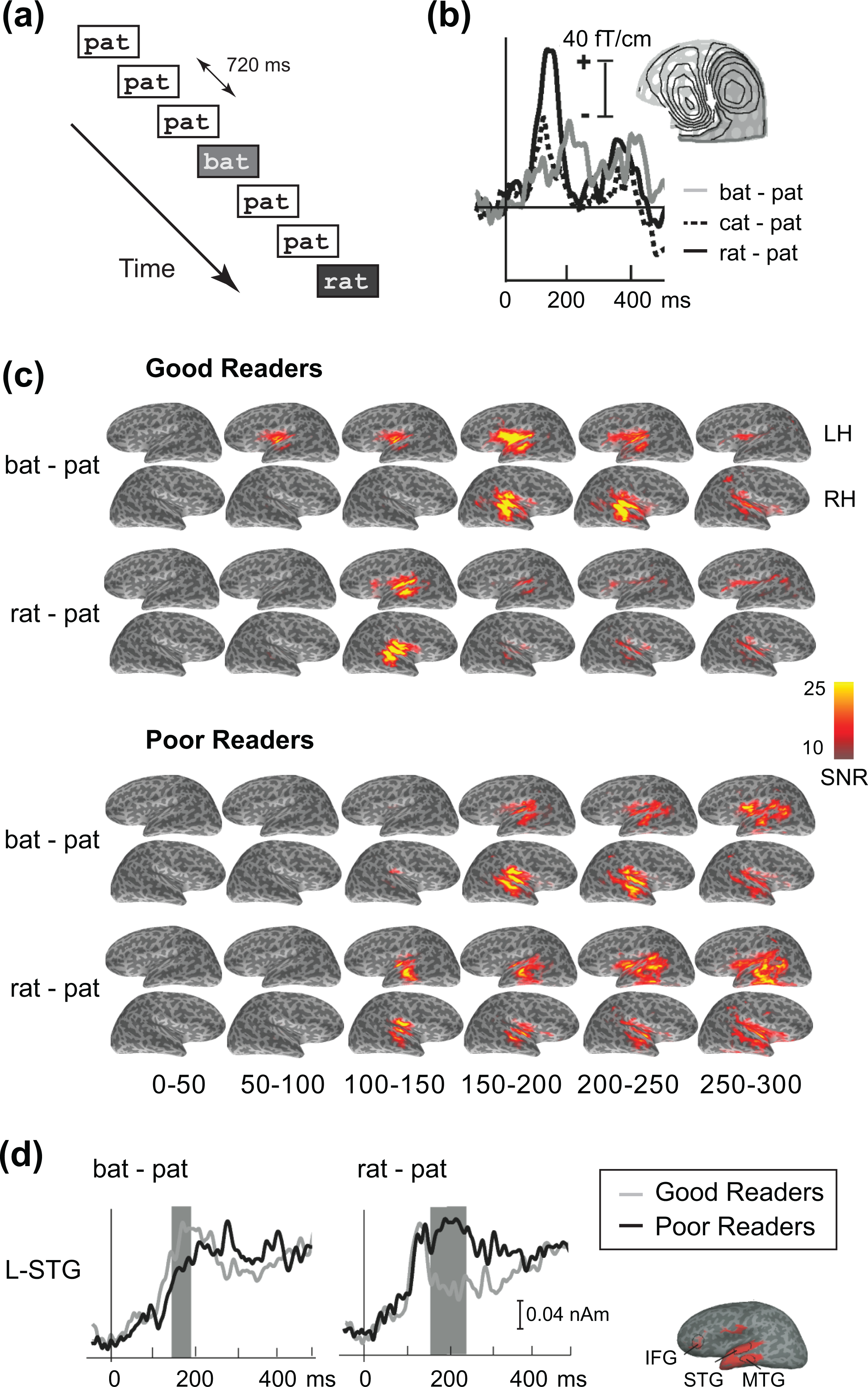
Spatiotemporal patterns of cortical activity revealed by MEG in a cognitive task. (a) Auditory discrimination paradigm. (b) Averaged time courses of auditory event-related magnetic field in a single left-hemisphere MEG sensor for one subject under three contrast conditions. (c) Distributed MEG source estimates of left and right hemisphere (LH, RH) responses to auditory contrasts in normal and dyslexic readers. Each map shows the mean value over a 50-ms time window. (d) Estimated source waveforms for the left hemisphere superior temporal gyrus (L-STG) region of interest (ROI). Time points at which significant differences between the conditions were found are indicated by shading. Adapted from Wehner et al. (2007).
Figure 4c depicts the sequences of estimated event-related cortical activity. Condition and group specific differences were evident in the superior temporal cortex at several latencies. For the statistical testing of group differences, spatial ROIs as well as time windows of interest were identified on the basis of omnibus data in which the MNE solutions for all deviant conditions were averaged across all subjects. Six ROIs were chosen according to the spatial pattern of activity in the omnibus condition, labeled STG (superior temporal gyrus), MTG (middle temporal gyrus), and IFG (inferior frontal gyrus) in the left and right hemispheres. For time windows of interest, three 50-ms windows were selected around the peaks in the omnibus condition time courses for the ROIs: 65-115, 140-190, and 190-240 ms. Significant differences between the two subject groups were found in the left-hemisphere STG ROI at the 140-190 and 190-240 ms time bins (Figure 4d). Specifically, compared with good readers, the poor readers showed greater left hemisphere activation in the phonologically dissimilar (and more contrastive) rat-cat condition, but reduced left hemisphere activation to the phonologically similar (and thus less contrasting) bat-pat condition (in which the initial phonemes differ in one phonetic feature only, viz., voicing), reflecting their difficulties with phonological processing.
Overall, the study illustrates the use of sensor and source space analyses of MEG data, visualization of estimated sequences of cortical activity with anatomical MRI data, and analysis of amplitude measures obtained from spatial ROIs and latency windows.
Gamma-Band Phase Locking Modulated by Phonological Conflict During Auditory Comprehension
The second example demonstrates the analysis of oscillatory activity and functional connectivity between cortical areas, observed under competing phonological and semantic processing demands (Han et al., 2012). In this study, 10 good and 10 poor readers, 16 to 18 years of age, performed an auditory sentence comprehension task while MEG was recorded. The subjects heard spoken sentences in which the last word (“critical word”) was manipulated to create semantically incongruent words that were either phonologically similar (PS) or phonologically dissimilar (PD) to the corresponding congruent (C) critical words (Figure 5a). The subjects had to indicate whether the sentences made sense or not by pressing one of two buttons.
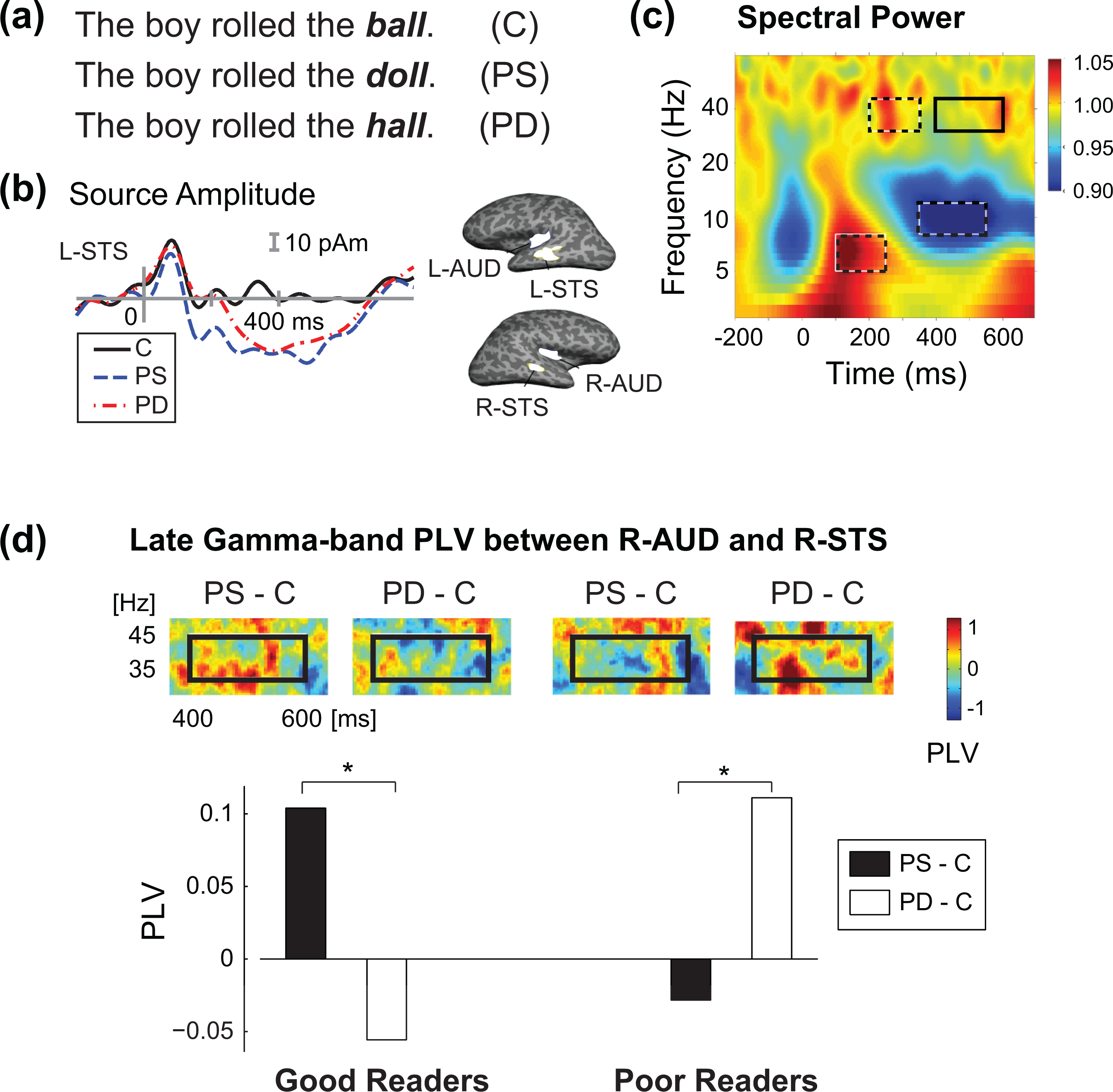
Analysis of oscillatory activity and functional connectivity among cortical regions using MEG. (a) Examples of spoken sentences with congruent (C) and incongruent (PS—phonologically similar to the congruent word, PD—phonologically dissimilar) critical word at the end. (b) Event-related MNE source waveforms in response to the critical word in a spoken sentence comprehension task for four regions of interest (ROIs; L—left, R—right, AUD—auditory cortex, STS—superior temporal sulcus). (c) Wavelet-transformed time-frequency representation of the event-related power spectrum averaged over all subjects and experimental conditions. (d) Phase-locking values (PLV), measuring functional coupling between the two right-hemisphere ROIs, shown for two subject groups and two experimental conditions in the late gamma band (400-600 ms, 30-45 Hz) time-frequency window. Adapted from Han et al. (2012).
Averaged event-related activity in one subject in response to the three types of critical words is depicted in Figure 5b. Cortical ROIs were determined on the basis of an omnibus source activation map obtained by averaging noise-normalized MNE solutions across all subjects and conditions over the time window of 200-500 ms. Four ROIs were identified, labeled AUD (for auditory cortex) and STS (superior temporal sulcus) in each hemisphere. The time courses depict the estimated source waveforms (MNE) for the three conditions (C, PS, PD) in the left hemisphere STS ROI; note the prominent response to incongruent words at a latency of about 400 ms, corresponding to the well-known N400 event-related potential component in EEG. The time-frequency power spectrum, relative to the prestimulus baseline, in response to the critical words, averaged over all subjects, stimulus conditions, and the four spatial ROIs is shown in Figure 5c. The event-related spectral power was increased around 100 ms in the 6-9 Hz frequency range, and decreased at 300-600 ms around 10 Hz (event-related desynchronization in the alpha band). Increased oscillatory activity was seen at 40 Hz (gamma band), most prominently around 200 and 600 ms. Based on this omnibus power spectrum data, four time-frequency windows of interest were selected for statistical analysis.
Functional connectivity between cortical areas was evaluated using the phase locking value (PLV), which is a measure of phase coherence between two oscillatory signals (Lachaux et al., 1999). Figure 5d shows the PLV measures between the two right-hemisphere ROIs in the late gamma time-frequency window (400-600 ms, 35-45 Hz). The data are shown separately for the two subject groups (good and poor readers) and subtracted stimulus conditions (PS-C, PD-C). The PLV was larger in the PS-C condition than in the PD-C condition in good readers, whereas the reverse was found in poor readers. These results may be indicative of the impaired phonological coding abilities of the poor reader group, and reflect its vulnerability under the perceptually demanding PS condition compared with good readers. The findings also support the role of gamma oscillations in spoken language processing.
In general, this study illustrates the use of MEG to study oscillatory brain activity and functional coupling of activity between cortical regions. It also highlights the potential use of MEG for understanding impaired cognitive processing. Interestingly, the N400 response, which indexes the robustness of a phonetic trace here, could provide a useful measure of the processing of contextual information within organizational settings (Braeutigam, 2014). In fact, the N400 has been found to reflect gender differences in decision making strategies (Braeutigam et al., 2004). The extent to which such differences in how one feels may be evident before the overt decision could provide useful insight into people’s behaviors for use in management training (Dhar & Simonson, 2003).
Summary and Conclusions
MEG provides excellent time resolution and good spatial resolution for revealing patterns of activation within and between networks of cortical areas in the human brain. As such, MEG is well suited to examine the subtle dynamics of cortical processes as they unfold spontaneously in resting state or over the course of a structured task. With a growing interest in big data, MEG is poised to make a rich contribution to the extraction of neural signatures of complex human behaviors in health and disease.
Footnotes
Declaration of Conflicting Interests
The author(s) declared no potential conflicts of interest with respect to the research, authorship, and/or publication of this article.
Funding
The author(s) disclosed receipt of the following financial support for the research, authorship, and/or publication of this article: The authors acknowledge the support from the National Institute of Neurological Disorders and Stroke (NS037462) and the Nancy Lurie Marks Family Foundation.