
Abstract
Theories are the core of any science, but many imprecisely stated theories in organizational and management science are hampering progress in the field. Computational modeling of existing theories can help address the issue. Computational models are a type of formal theory that are represented mathematically or by other formal logic and can be simulated, allowing theorists to assess whether the theory can explain the phenomena intended as well as make testable predictions. As an example of the process, Locke’s integrated model of work motivation is translated into static and dynamic computational models. Simulations of these models are compared to the empirical data used to develop and test the theory. For the static model, the simulations revealed largely strong associations with robust empirical findings. However, adding dynamics created several challenges to key precepts of the theory. Moreover, the effort revealed where empirical work is needed to further refine or refute the theory. Discussion focuses on the value of computational modeling as a method for formally testing, pruning, and extending extant theories in the field.
Theories of organizational and psychological phenomena are not only numerous and complex but also imprecise and rarely tested rigorously (J. R. Edwards, 2010). One means for adding precision and facilitating theory testing is via computational modeling (Adner, Pólos, Ryall, & Sorenson, 2009; Farrell & Lewandowsky, 2010). Computational models provide formal specifications of the components and processes of a theory. That is, the specifics of the functional forms or processes are represented mathematically or with propositional logic. The formality helps make the theory specification more transparent (Adner et al., 2009) and theory testing more rigorous (J. R. Edwards & Berry, 2010). They can also be simulated to determine if the components and processes proposed produce the phenomena that the theory intends to explain and which components are key (Davis, Eisenhardt, & Bingham, 2007). Moreover, the simulations predict trajectories or distributions for constructs over time (e.g., Vancouver, Li, Weinhardt, Purl, & Steel, 2016) and can predict relationships that can be tested in empirical investigations (Vancouver, Tamanini, & Yoder, 2010). The models themselves can be fit to empirical data to assess model fit (e.g., Vancouver, Weinhardt, & Schmitt, 2010) and more importantly, compare alternative models (Farrell & Lewandowsky, 2010; Vancouver & Scherbaum, 2008). Indeed, the value of computational modeling has long been recognized in cognitive psychology (Busemeyer & Diederich, 2010) and macro-organizational theory (Lomi & Larson, 2001; Prietula, Carley, & Gasser, 1998; Simon, 1969) but is also beginning to transform micro- and meso-organizational research areas like multiple goal pursuit (Vancouver, Weinhardt, et al., 2010) and team processes (Grand, Braum, Kuljanin, Kozlowski, & Chao, 2016).
Yet the use of computational modeling within the field is still very limited. In part, this may be because it is difficult to comprehend the advantages of computational modeling noted previously without seeing those advantages realized in specific cases. Moreover, observing the process of creating models likely helps one see how to do it. Toward that end, we provide such an example here using two modeling platforms: Vensim and Matlab. 1 Finally, a third issue possibly limiting the use of computational models is difficulty knowing what to model. Some argue that one should use models to create new theory, which is challenging in and of itself (e.g., Davis et al., 2007). However, others argue that formally modeling existing nonformal theories is actually the better place to start and much needed (Busemeyer & Deiderich, 2010; Farrell & Lewandowsky, 2010; Vancouver, Tamanini, et al., 2010). In particular, they note that one advantage of modeling existing theories is that the process often lays bare the elements of the theory that are underdeveloped, which requires some theory development in its own right. For example, many theories in organizational behavior are presumed to describe the processes by which things change, but many are static in nature (e.g., provide no description of the rate of processes), and it is not clear that the translation to a dynamic theory would be straightforward. Thus, the process of translating an existing nonformal theory to a computational model is likely to motivate refinement as well as highlight the need for additional empirical work, which is one of the primary roles of good theory (J. R. Edwards, 2010).
Moreover, Farrell and Lewandowsky (2010) argue that translating current theories into computational models is necessary for vetting the theories, particularly when they are complex, and facilitating strong inference via theory comparison. Such vetting may help “prune” organizational science’s “dense theoretical landscape” (Leavitt, Mitchell, & Peterson, 2010, p. 644). Beyond removing or improving existing theory, computational modeling can also highlight the overlap among different theories and/or the linking of theories to meta-theories. For example, Vancouver, Weinhardt, and Vigo (2014) showed that information processing involved in goal striving, goal choice, and supervised learning could be represented via the same mathematical function. Given J. R. Edwards’s (2010) assessment of the state of theory, it seems the assessment, refinement, integration, or elimination of current theory would be a useful enterprise for organizational scientists and one that computational modeling could substantially facilitate.
Toward this end, we wish to provide an example of the process of translating a nonformal theory into a computational one. In particular, we take part of a well-established, complex, and presumably practically useful theory in organization behavior and vet it computationally. This theory, called the integrative model of work motivation (IMWM; Locke, 1997; Locke & Latham, 2004), is an integration of goal-based (e.g., social cognitive theory, Bandura, 1997; goal theory, Locke & Latham, 1990) and other motivational theories (e.g., expectancy theory, Vroom, 1964). Moreover, this integrative theory has begun to inform subsequent theorizing within the field (e.g., Meyer, Becker, & Vandenberghe, 2004; Rose & Manley, 2011) and has the potential to play a major role in the future of work motivation research (Locke & Latham, 2004; Nahrgang et al., 2013). However, the IMWM is largely represented as a path diagram model (partially reproduced in Figure 1) and employs a set of verbal descriptions of its theoretical processes (e.g., Locke & Latham, 1990, 2002). Critically, the “model is static, not dynamic” (Locke & Latham, 2004, p. 391). Yet Locke and Latham endorsed translating the IMWM into a dynamic model and included a feedback loop in the model (i.e., indirect links from self-efficacy to performance and a direct link from performance back to self-efficacy). They also cited a study by Mone (1994) that presumably showed that the static model would generalize to a dynamic context.
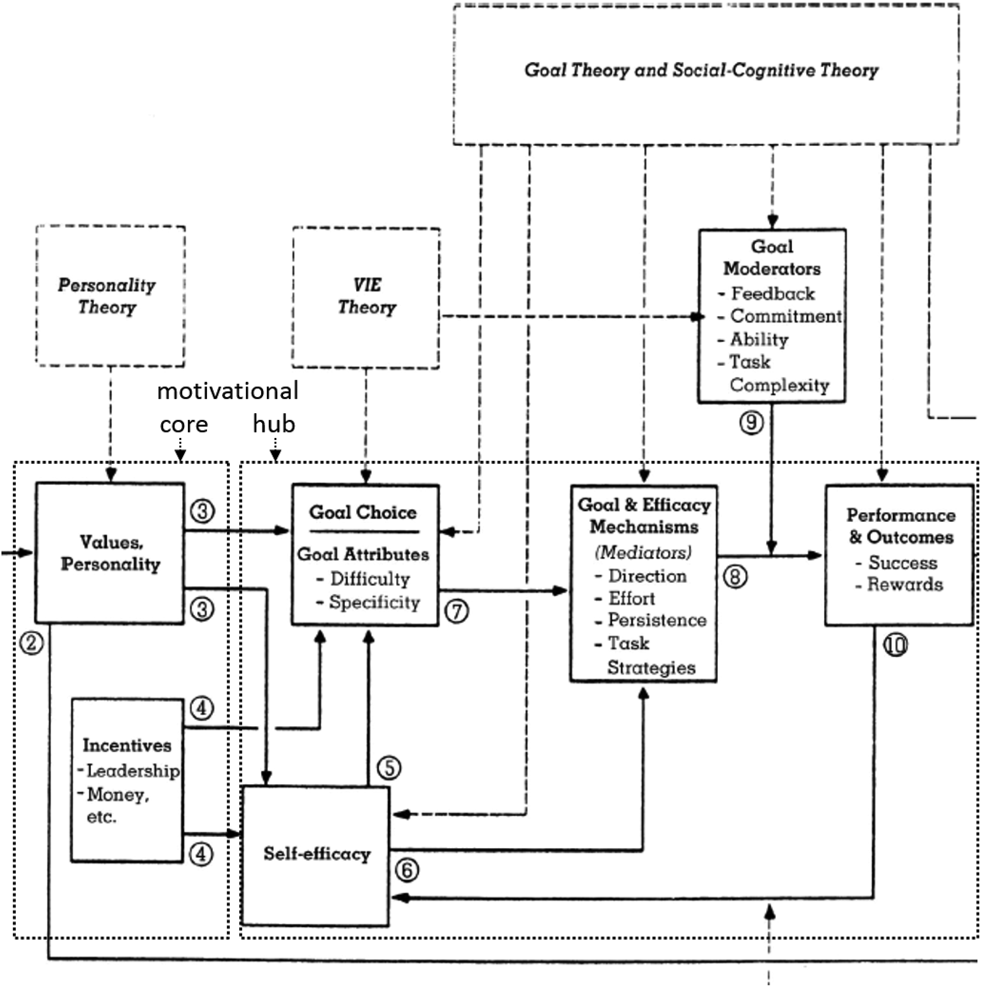
Partial reproduction of integrative model of work motivation (IMWM).
However, understanding the implications of dynamic processes are far more complicated than they are for static models because it is often difficult to envision the exact implications of dynamic processes over time (Cronin, Gonzalez, & Sterman, 2009; Farrell & Lewandowsky, 2010). This is where formal computational models are especially useful (DeShon, 2012, 2013; Hanges & Wang, 2012; Ilgen & Hulin, 2000; Kozlowski, Chao, Grand, Braun, & Kuljanin, 2013; Vancouver & Weinhardt, 2012; Wang, Zhou, & Zhang, 2016). Otherwise, it is often not clear if a nonformal theory can exhibit the internal consistency necessary to make valid conclusions given humans’ propensity for making logical errors when considering dynamic processes (Cronin et al., 2009). Because of this, we argue that the static and dynamic versions of the IMWM should be vetted computationally to assess their viability and merit.
Given the previous discussion, our objective was to begin to translate the IMWM into a dynamic computational representation that could be simulated to assess its internal consistency and highlight the components that are underdeveloped or need empirical examination. To accomplish this, we first needed to confirm that a static computational model could represent and reproduce the results used to create the static model. Of course, as is typical during the process of translating a nonformal model into a computational one, we found some need for model elaborations (Busemeyer & Diederich, 2010; Davis et al., 2007). In some cases, these elaborations could be gleaned from the writings of Locke and Latham (e.g., Locke & Latham, 2002) or empirical and theoretical work on work motivation (e.g., Latham & Baldes, 1975; Locke, Shaw, Saari, & Latham, 1981; Vroom, 1964). Indeed, the empirical work served as referents for the results of our simulations. For example, we used a classic longitudinal study by Latham and Baldes (1975) as an empirical referent for our dynamic model. To foreshadow our results, we found that we could create viable static and dynamics computational models, but simulations and experiments with them created several challenges to various aspects of the represented theory.
The paper is organized as follows. First, we review the merits of and processes involved in computational modeling as well as the IMWM and the theories it integrates. This is followed with the development of the formal static representation of the IMWM. In this development process, considerable attention is paid to internal validity, which in the computational modeling community refers to the degree to which the model corresponds to the theory it is supposed to represent (Taber & Timpone, 1996). We assess the static computational model by simulating it and comparing the results it generates against existing empirical findings. That is, we determine if our model can produce the phenomena the nonformal theory purports to explain. We also use the computational model to identify the key processes involved in explaining the phenomena. We then added a dynamic element to the model as suggested by Locke (1997). Nonetheless, the lack of guidance from the IMWM on the dynamic features required considering different mechanisms. This provided an opportunity to illustrate how computational modeling can facilitate theory development (Davis et al., 2007). To assess the dynamic model, we sought to produce via simulation a result similar to the referent empirical finding (Latham & Baldes, 1975). Finally, we discuss the implications derived from the modeling efforts and how the process can be used to further develop theory computationally, conceptually, and empirically.
On the Value of Computational Modeling
Theories are expressed with words (i.e., verbal theories), graphics (e.g., path diagrams, grids), mathematics, or other logics (Adner et al., 2009). Graphics and mathematics are more universal than words, which are language specific. However, both can obscure details depending on the level of abstractions represented and the specific types of representations. For example, path diagrams tend not to indicate the form of the relationships (i.e., they imply linear relationships, though exceptions exist; e.g., Naylor, Pritchard, & Ilgen, 1980), and even math can be vague. For example, B = f [P, E] merely means behavior is a function of person and environment; the function is left unspecified. On the other hand, computational models require explicit equations that define the functional forms for relationships between causes and effects. 2 These explicit equations provide transparency, precision, and the capacity for model simulation. Simulations in turn indicate whether the model is mathematically coherent (e.g., no simultaneous equations). Once mathematically coherent, simulations of the model allow the theorist to confirm that the theory accounts for the phenomena it purports to explain and make predictions that can be compared with empirical data. In particular, when dealing with theories of dynamic phenomena, model simulations often generate unexpected outputs (Hintzman, 1990), motivating further refinements of the theory (Davis et al., 2007; Wang et al., 2016).
To create computational models, Vancouver and Weinhardt (2012) described several steps. The first is to define the problem. They, like others (Busemeyer & Diederich, 2010), suggest that models can be made to represent a core aspect of existing nonformal theory. In the current case, we mainly focused on the motivational hub and motivational core of the IMWM (see Figure 1; Locke, 1991), a mediating construct within the hub (i.e., effort), and the moderators that affect the processes presumably operating within the hub. This motivational hub also includes the feedback loop that forms the basis of the dynamic element.
The second step is to define the system boundary to be modeled (Vancouver & Weinhardt, 2012). In this case, we excluded constructs and processes that affect constructs and processes prior to and after the motivational hub/core, making the modeling focused and succinct. If the modeling proves viable, the possibility of adding the other components could be considered. In addition, the system is bounded by the features that define the IMWM (e.g., IMWM describes the process of single goal pursuit). Moreover, the IMWM is primarily a model of goal choice (i.e., the level of personal goal one chooses to pursue) and the effect of that choice on performance over days, weeks, or longer timeframes. That is, it does not attempt to explain the fine-grained processes that lead to a level of performance for a single goal-striving episode. Nonetheless, computational models of this lower level of explanation exist (e.g., Vancouver & Purl, 2017) and informed the modeling constructed here. When such links are made, we reference this other work. The final two steps of modeling include building the model and evaluating it. These steps represent the bulk of the work described here.
One caveat for computational theorists who build models of other scholars’ theories is that the modelers might not have properly represented the theory. For this reason, it is important for modelers to “show their work” when building the model (i.e., show and justify each function in the model). In this way, others can evaluate the reasoning used to construct the model and the simulation results that motivate revisions or specifications (Busemeyer & Diederich, 2010). Moreover, most models are intended to represent processes occurring with entities (e.g., humans, teams, or organizations). When this is the case, the realities of the constraints on the entities need to be considered when constructing the models. That is, math is more flexible than the entities, which must adhere to physical and informational limitations. Computational models are more likely to be a valid reflection of the entities not only when using existing theories to create the models but also when required to explain why specific constructs and functions are used.
For example, one challenge we faced modeling the IMWM was that many of its constructs are multidimensional. This means that although the dimensions within a construct appear to deserve enough consideration to be distinguished from the other dimensions within the same construct, they are not distinct enough to deserve a particular set of causes or effects in the pictorial description of the theory. That is, one directional path (i.e., arrow) traversing between two multidimension constructs (e.g., goal choice to goal mechanisms) represents the notion that all the dimensions of a construct presumably cause (or moderate) all the dimensions in the affected construct in the same way. This facilitates a parsimonious presentation, but it could raise issues when building the computational model. To address these issues, we either focused on what we thought was the most important or well-considered dimension within a construct or separated the dimensions into multiple constructs. To facilitate this process, we used verbal statements by Locke (1997) or Locke and Latham (1990), empirical findings, or precepts from the theories represented in the IMWM. The use of empirical findings is consistent with the inductive approach to theorizing used to develop the IMWM and several of the theories integrated within it (Locke, 2007). In the next section, we briefly review these theories.
Brief Review of IMWM and Its Theoretical Foundations
The IMWM was introduced in a chapter by Locke (1997) and reiterated in an Academy of Management Review paper with Latham (Locke & Latham, 2004). The IMWM is largely a depiction of what constructs affect what other constructs and is thus primarily communicated via a path diagram (Locke, 1997, p. 402; Locke & Latham, 2004, p. 390). The path diagram, reproduced in part here (see Figure 1), shows which constructs cause or moderate the effects of other constructs via arrows representing direction of causality. Moreover, “the model in this figure is not speculative but is, with one exception, entirely empirical” (Locke, 1997, p. 401). The one exception is the link from needs to values, which is not shown in Figure 1 because it is outside the boundary we consider here. Indeed, Locke and Latham (2002, 2004) were particularly confident with the empirical support for what they called the motivational hub (see Figure 1). The hub includes the key attributes of goals within the goal choice construct (i.e., difficulty and specificity), self-efficacy, and performance. An important boundary of the theory, and thus of the models we built, is that performance refers to the single dimension defined by the goal referenced in the goal choice construct (e.g., number of widgets produced). The IMWM does not address processes where multiple goals or dimensions of performance are involved (Locke & Latham, 2004).
Locke (1997) also notes in a footnote to the figure that some arrows are omitted (e.g., self-efficacy affects commitment), complexities related to the theories underlying the model are not fully elaborated, and recursive effects are not shown except for the self-efficacy–performance relationship. This type of filtering is common in nonformal theory presentations for the same reason computational modelers often circumspect the complexity of the models they build: concern for information overload of the reader. However, unlike the nonformal theory representation, a computational modeler will need to include elements that allow for a coherent, working whole (Busemeyer & Diederich, 2010). In this case, we needed a few more constructs and links in the IMWM beyond the motivational hub.
First, we included values/personality, which Locke (1991) calls the motivational core or essence of motivation because some positive anticipated value for a behavior or goal is necessary for motivation. Thus, we included a value construct to represent this notion. We also included one of the dimensions within the goal mechanism (i.e., effort) 3 that mediates the effects of goals on performance according to the IMWM. Finally, we added the goal moderators (i.e., feedback, goal commitment, ability, and task complexity) given their role in determining the degree of the goal effects on performance and the inclusion of goal commitment in some descriptions of the motivational hub (e.g., Locke & Latham, 2002). However, we separate these moderators into two sets, depending on the process they moderated. That is, because the lack of feedback and goal commitment undermine goal-directed effort, we shifted the moderating effect of these constructs to goal mechanisms (i.e., effort). In contrast, ability and task complexity affect the degree to which applied effort affects performance, which is consistent with the location of the moderation illustrated in Figure 1.
To explain the relationships depicted and provide some insight into how causes are combined to determine the value of a variable, the IMWM draws on multiple theories (see dashed boxes in Figure 1). These include goal theory (Locke & Latham, 1990; Ryan, 1970), social cognitive theory (Bandura, 1986), and VIE (valence, instrumentality, expectancy; Porter & Lawler, 1968) theory, which is derived from expectancy theory (Vroom, 1964).
Goal Theory
Goal theory was developed from a theory articulated by Ryan (1970) and augmented based on empirical findings (for an introduction of the theory and extensive review of the empirical literature related to the theory, see Locke & Latham, 1990). The primary empirical findings included the observation that those assigned (i.e., asked to adopt) difficult goals tended to perform better than those assigned easier goals, where goal difficulty refers to the level of the goal (e.g., number of widgets to complete). Indeed, a common depiction of the core of goal theory is shown in Figure 2 (e.g., Locke & Latham, 1990, 2002). It shows that assigned goals affect personal goals and self-efficacy, both of which affect performance. Interestingly, this figure also appeared in the chapter where Locke (1997) introduced the IMWM and represents some important constructs not as clearly represented in the IMWM—a point we return to in the following.
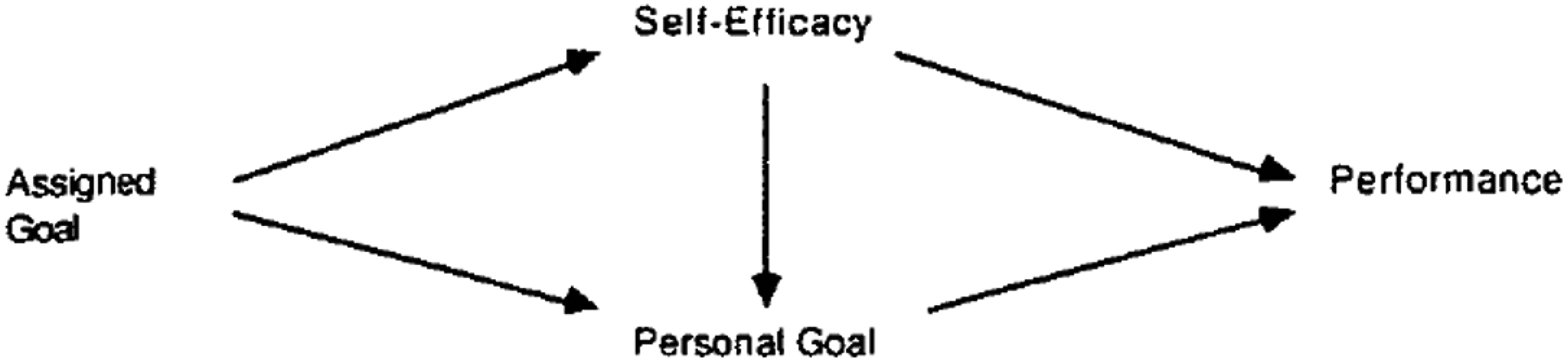
Relationship between assigned goals, personal goals, self-efficacy, and performance.
In addition to the effect of goal difficulty, another set of empirical findings included the observation that those assigned a difficult goal outperformed those assigned a “do-your-best” goal or no goal. This distinction between an assigned goal and no assigned goal level is called goal specificity, where the do-your-best or no goal specified are two ways to operationalize low goal specificity and the assignment of a difficult goal is how high goal specificity is operationalized. In more recent years (Locke & Latham, 2002), goal specificity is described as a variable that reduces variance in performance rather than a cause of performance.
While developing the empirical basis for goal theory, several moderators were uncovered, including the person’s ability, presence (or absence) of external feedback on goal progress, goal commitment, and complexity of the task. Specifically, the effects of goal difficulty and specificity on performance are weaker when ability is low, external feedback is absent, goal commitment is low, and complexity of the task is high (Locke & Latham, 1990, 2002).
Social Cognitive Theory
IMWM was also heavily influenced by Bandura’s (1986) social cognitive theory (SCT). SCT assumes that individuals use forethought before adopting goals and engaging in behavior. A key aspect of forethought involves beliefs regarding valued outcomes associated with the behavior or performance and beliefs in one’s capability to engage in the behavior or achieve given levels of performance. This latter belief is referred to as self-efficacy (Bandura, 1997). According to SCT, self-efficacy positively relates to the likelihood one will adopt a goal, amount of effort one exerts while pursuing an adopted goal, and length of time that effort is applied (i.e., persistence).
VIE Theory
VIE or expectancy theory also assumes that behavior is a function of one’s beliefs regarding the value of the outcomes one expects to obtain from engaging in the behavior (Vroom, 1964). Moreover, VIE is a formal mathematical theory of work motivation in that it specifies a function for motivation. Specifically, motivational force (MF) is the outcome of multiplying one’s belief that behavior will lead to performance (i.e., expectancy; E) by the sum of one’s beliefs that performance will lead to various outcomes (i.e., instrumentality; I) times the anticipated value (i.e., valence, V) or satisfaction of obtaining those outcomes (i.e., MF = E × ∑Io × Vo). Finally, the theory states that choice (i.e., direction) is a function of comparing motivational forces across behavioral options (e.g., engaging or not engaging in the behavior), and effort and persistence on the option chosen are positive functions of motivational force.
The relationships among goal, SCT, and VIE theories in the IMWM are not completely clear. That is, goal theory and SCT were included in a single dashed box in the model, a box that was implicated in several processes within the model. VIE had its own box, but the two constructs it points at are also pointed at by the goal theory/SCT box. This is not necessarily problematic. Indeed, in the spirit of an integrative effort, it appears that IMWM assumed overlap among the theories and that empirical work motivated by any or all the theories described might inform the larger, final integrative model. For example, the motivational force equation found in VIE seems a mathematical operation of SCT’s view of how these constructs affect motivation and was itself derived from decision theories (e.g., W. Edwards, 1954). In this way, the formality reduces the overlap, or redundancy, among the theories.
Building and Evaluating the Static Model: The Motivational Hub/Core
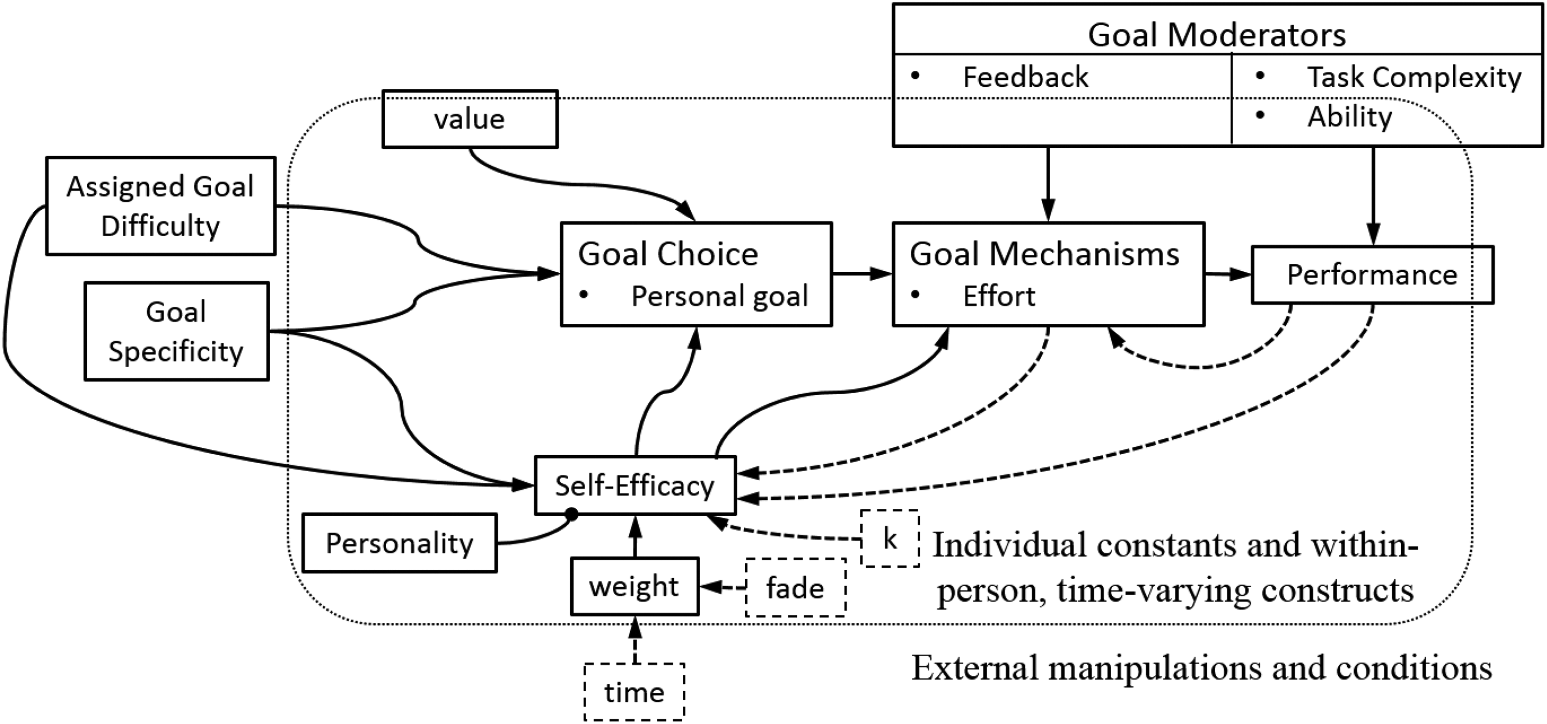
In this section, we specify the exact exogenous and endogenous variables we used for the static model, which is depicted in Figure 3. Exogenous variables are variables not caused by other variables (i.e., constructs) represented within the model, and endogenous variables are affected by other variables in the model. For example, exogenous variables might be manipulations used in developing and testing a theory, and the endogenous variables might be key psychological mediators and behavioral outcomes.
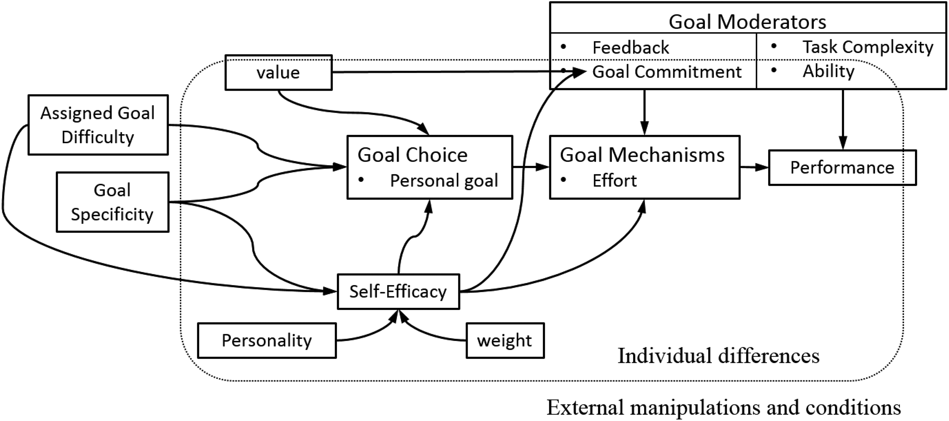
Static computational model of the core of the integrative model of work motivation (IMWM).
We begin our model building by specifying the exogenous variables. However, some explanation of the conventions used to create Figure 3 is needed. For example, similar to depictions of statistical models, we include weights for the effect of one variable on another. What might seem surprising is that we only have one such weight in Figure 3, which is used to represent the effect of assigned goal difficulty on self-efficacy and we conveniently labeled weight. Given that weights tend to be free parameters when assessing the fit of models to data and the number of free parameters reduces the predictive value of a model (Myung, 2000), it behooves the modeler to begin with as few such parameters as possible (Heathcote, Brown, & Wagenmakers, 2015). Indeed, in terms of theory building, one should only add a parameter if one has reason to believe the input is somehow mitigated or enhanced. That is, rather than assume a weight that might be removed later, assume no weight and add if needed. 4
Another convention used in Figure 3 that is typical of representations of computational models relates to moderators. The primary issue is that input variables can serve several possible roles in a function (e.g., power term) beyond the narrow notions of main effect or moderator. Thus, the convention in diagrams of computational models is to point any variable that is used in an endogenous variable’s function at the endogenous variable directly (Vancouver & Weinhardt, 2012). For this reason, moderators point at the endogenous variable affected by the moderated input as opposed to the arrow from the input variable. We should note that we do not use symbols to represent the nature of the links (e.g., positive, negative, multiplicative) because these symbols do not always fully communicate the functional forms (i.e., the equations) used in the model. Rather, the code for the model, often presented in an appendix or a table like Table 1, is needed to be fully transparent regarding the model and its functions. Indeed, modelers should make their models available to researchers so others can download, examine, and simulate them. In the present case, the model is coded in Vensim as well as Matlab (see Appendices A and B, respectively). A version of Vensim software that can simulate the model can be downloaded for free if being used for educational or academic purposes, 5 and many universities have licensing agreements for Matlab. 6
Constructs and Functions of the Static and Dynamic integrative model of work motivation (IMWM) Models.
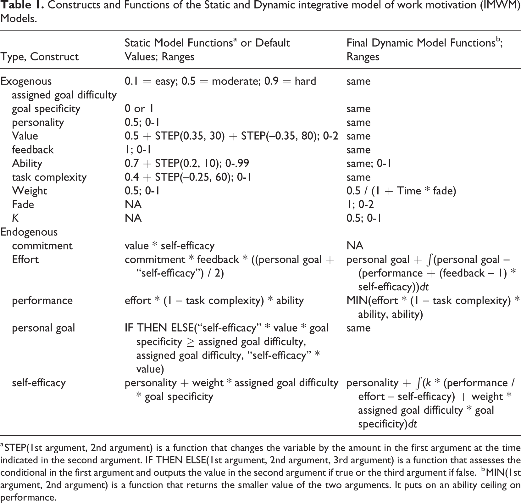
a STEP(1st argument, 2nd argument) is a function that changes the variable by the amount in the first argument at the time indicated in the second argument. IF THEN ELSE(1st argument, 2nd argument, 3rd argument) is a function that assesses the conditional in the first argument and outputs the value in the second argument if true or the third argument if false.
b MIN(1st argument, 2nd argument) is a function that returns the smaller value of the two arguments. It puts on an ability ceiling on performance.
Finally, we did one unusual thing regarding Figure 3 in terms of computational modeling convention. To facilitate the link between our model and the IMWM, we included both process and construct labels in a few cases. For example, goal choice is a process that determines the level of the personal goal construct, and feedback (i.e., construct) is a moderator (i.e., process). With these issues addressed, we proceed to explaining the model.
The Exogenous Variables
The static computational model included eight exogenous variables. Most of these are clearly represented as such in the motivational hub of the IMWM, but some are not. Table 1 lists all the variables in our initial static model. It also provides the functions or default values used in the simulations.
Assigned Goal Difficulty and Goal Specificity
When operationalizing the IMWM computationally, we represent assigned goal difficulty and goal specificity exogenously. Labeling these variables exogenous might at first appear to be inconsistent with the IMWM shown in Figure 1 given that difficulty and specificity are attributes within the goal choice construct and values, personality, incentives, and self-efficacy are constructs that point at the goal choice construct (i.e., goal choice is endogenous). Yet our choice to set the motivational hub as a boundary of our model and the empirical strategies used to develop the motivational hub dictate this change. Specifically, Locke and Latham (2002) described assigned goal difficulty as an element of “leadership” within the “incentives” construct, and incentives are an exogenous variable in the IMWM (see Figure 1). Moreover, as noted previously, a primary manipulation used to test goal theory was to assign goals of varying difficulty. Manipulations are by definition exogenous. Likewise, Locke and Latham (2002) note that leaders might or might not assign goals and that the assigning or not of a specific goal level was another major manipulation used to develop goal theory (Locke & Latham, 1990). Thus, goal specificity appears to be another element of the exogenous construct. Here, goal specificity is separate from assigned goal difficulty because it represents a different type of manipulation. Note the goal choice construct within IMWM appears to refer to internal properties of the individual (Locke, 1991). In particular, the goal attribute of difficulty refers to a property of the personal goal held by the individual (see Figure 2). For this reason, we relabeled the construct within goal choice personal goal. It refers to the level of difficulty of an accepted or self-set goal. We also place this construct within the box that distinguishes person constructs from environmental constructs (i.e., external manipulations and conditions), though in some cases (i.e., values and performance), the constructs cross this boundary, which is also depicted in Figure 3.
Besides specifying the exogenous variables, computational modelers can provide scales for these variables to make more specific point predictions. As a manipulation, assigned goal difficulty is typically operationalized in terms of the percentage of individuals in the population of interest who could achieve the level of performance on the goal in question (e.g., make 20 widgets). An easy goal is one that could be achieved by those at or above the 10th percentile, whereas a hard goal is one that could only be achieved by those at or above the 90th percentile (Locke & Latham, 1990). Given this, we scaled assigned goal difficulty in percentiles, where 0.1 represents an easy goal, 0.5 a medium goal, and 0.9 a hard goal. For goal specificity, studies nearly always manipulated it by assigning one group a specific level of performance (e.g., a hard goal) to achieve and another group a do-your-best or no goal (Locke et al., 1981). Thus, in our model, goal specificity could take on two values: zero for the no goal or do-your-best condition and one when a specific goal is assigned (see Table 1).
Value
It is not completely clear what value means in the IMWM. However, it appears that value is a determinant of personal goals and goal commitment as described in theories like VIE or SCT. That is, one key value would represent the attractiveness or importance of performance on the dimension of interest (e.g., widgets made). This value may be a function of external incentives, like when monetary incentives are provided for performance combined with the notion that individuals tend to value money (Locke, 1997). For our purposes, we initially assume that value is a variable that can range from 0 to 2, where 2 represents a maximum anticipated positive value or attractiveness associated with this dimension of performance. In the simulations considered here, like most of the empirical work, we assume the goal, and thus goal performance, is positively valued. To be sure, negative valued goals likely exist, but they would create additional computational complications, so this will be a boundary to our model. Moreover, we do not take a position on the reason for the value being assigned to the goal. That is, it may be via associations set up externally or internally. Thus, the construct sits on the boundary between individual differences and external manipulations and conditions in Figure 3.
Personality
Personality may be another indicator of the values an individual holds (Locke & Latham, 2002), making it redundant—and perhaps reasonably combined in one construct as done in the IMWM. However, within the IMWM, personality is also considered to be an individual difference variable that affects one’s self-efficacy. Because computational modeling requires clearly distinguishable inputs and outputs, we use personality only for the purpose of indicating self-efficacy propensity. Given that use, we scaled personality in terms of self-efficacy, which we scaled in terms of a performance level one thinks one is capable of reaching and where performance is scaled in terms of percentiles like goal level. As noted in Table 1, the default value for personality in the simulations presented was 0.5, though we used the full range of values during the sensitivity analysis summarized in the model evaluation section below.
Feedback, Ability, and Task Complexity: The Exogenous Moderators
Feedback, ability, and task complexity are all exogenous moderator variables in the IMWM. The other goal moderator, goal commitment, is caused by other variables included in the model as described verbally (e.g., Locke & Latham, 1990), and thus we describe it with the endogenous constructs. In goal-setting studies, feedback is usually operationalized as present or absent and the findings are that goal setting effects are stronger when feedback is present (Locke & Latham, 1990). Typically, presence to absence is scaled one to zero, but feedback is a complex construct (e.g., feedback could refer to information about a task state that one could observe directly or via another; it could be normative or absolute). Indeed, some computational modeling has been done regarding feedback (Vancouver & Purl, 2017) but is beyond the scope of what we want to accomplish here. Thus, we only consider high, unambiguous feedback (i.e., feedback = 1) in the simulations presented.
In contrast, ability plays an important role in the processes examined here, particularly when we get to the dynamic model. We generally scaled ability like we scaled personality and assigned goal difficulty. That is, we scaled it in terms of percentile of the population of performers. Thus, a high-ability person might be able to reach the 90th percentile, whereas a low-ability person might only be able to reach the 10th percentile. Other scales are possible, but they would need to be propagated throughout the model (e.g., if number of widgets made was the scale, self-efficacy and thus personality would need to be scaled in terms of number of widgets one would make in some specified period of time).
The final exogenous moderator is task complexity, which is the objective difficulty of the task. That is, it is an external property of the task, not a property of the person like ability, though it along with ability determine the individual’s capability for the task. Specifically, goal-setting research finds that task complexity moderates the effect of goal level on performance (Locke & Latham, 1990). We scaled this variable to be between 0 and 1 where 1 is the most complex a task can be and 0 the least complex. Given that task complexity and ability will modify the effect of effort on task performance, we refer to their combination as capability, though we do not explicitly separate this construct from the performance function. Finally, the last exogenous variable, weight, is better explained in terms of the description of factors and function that affects self-efficacy, which is an endogenous variable. Thus, we turn to these next.
The Endogenous Variables
All variables or constructs determined by other variables or constructs in the model are considered endogenous. These include self-efficacy, personal goal, goal commitment, effort, and performance. They are considered a function of the variables pointing at them (see Figure 3).
Self-Efficacy
In the static version of the IMWM, self-efficacy is a function of personality and assigned goal difficulty when a goal is assigned (Locke, 1997; Locke & Latham, 1990). The IMWM does not specify how personality determines self-efficacy, but here we simply have personality represent one’s initial level of self-efficacy for the task under consideration. Assigned goal difficulty was included because it has been found to positively affect self-efficacy (e.g., Earley & Lituchy, 1991; Gellatly & Meyer, 1992). Presumably, this is because difficult goal assignments signal confidence that the individual can perform at that high level (Bandura, 1997). Thus, we specified assigned goal difficulty and goal specificity as antecedent variables of self-efficacy so that assigned goal difficulty can influence self-efficacy when assigned a goal (i.e., goal specificity = 1). Finally, the signaling effect of assigned goal difficulty is likely only a fraction of the value represented in the assigned goal level. Thus, we included a weight, which was set to 0.5 for most of the simulations, to represent a medium effect for assigned goal difficulty on self-efficacy (see Table 1). These three inputs—assigned goal difficulty, goal specificity, and weight—were all multiplied by each other. Thus, when simulating a no assigned goal condition, goal specificity equals 0, and thus the product term is 0. In that case, self-efficacy is only based on personality.
Personal Goal
Arguably, the most important process within the motivational hub of the IMWM is the process that determines the individual’s personal goal (i.e., the level of performance one is seeking to achieve). As shown in Figure 1, incentives (e.g., leadership), values/personality, and self-efficacy are three constructs that influence goal choice (i.e., personal goal). Recall that we separated value from personality as well as assigned goal difficulty and goal specificity from the incentives construct. Given these modifications, the constructs (i.e., value, assigned goal difficulty, goal specificity, and self-efficacy) impacting personal goal appear to be straightforward interpretations of nonformal descriptions of the theory by Locke and Latham (1990, 2002). In contrast, the specific process by which these inputs affect personal goal is not explicitly articulated within the IMWM, goal theory, or SCT. Thus, it is not clear how we should combine these inputs. This lack of specification is not a debilitating problem though. Rather, it is an opportunity to show how computational modeling can make theoretical choices transparent and supporting text can be used to explain why the choices are made. Of course, the choices we made may not be correct in terms of (a) representing the processes involved within individuals or (b) representing the processes that Locke or Latham think are involved, but they are specific, clear, and computationally testable.
For personal goal, we suspect two processes might be involved: the process that determines whether to accept an assigned goal or not and the process that determines what will be one’s personal goal if the assigned goal is rejected or no goal is assigned. Thus, when a goal is assigned and rejected or no goal is assigned, a process for determining the internally represented personal goal level is needed. Toward that end, Locke and Latham (1990) noted that prior to goal-setting theory, researchers had identified “Two basic categories of determinants…namely expectancy of success and the valence (or value) or [sic] success” (p. 111). More recently, Klein, Austin, and Cooper (2009) noted that “nearly every theoretical perspective attempting to explain conscious goal choice (…Locke & Latham, 1990) uses an expectancy-value framework (e.g., Vroom, 1964)” (p. 111). Indeed, the two components of expectancy-value models, a belief regarding capability to realize the outcome (i.e., reach a goal level in this case) and the values associated with realizing the outcome, respectively, had acquired many labels over the years and across the theories that used them. By the time the IMWM was developed, Locke (1997) was using the term self-efficacy for expectancy given he considered it a broader concept and a better measure. Locke (1997) also appeared to prefer the label value to valence. Thus, self-efficacy and value are two of the key determinants of goal choice in the IMWM (as shown in Figure 1) and our model of it (as shown in Figure 3).
In terms of the specific role for value, we mentioned that the IMWM, goal theory, and SCT are not precise regarding how its effect might manifest. However, VIE theory, which Locke (1997) includes in the IMWM and points at the goal choice box (see Figure 1), offers a precise mathematical description of the process. Specifically, values associated with a goal are weighted by the self-efficacy of achieving the goal. This describes a multiplicative function (Vroom, 1964). Given that self-efficacies range from 0 to 1 and values from 0 to 2, the product will also range from 0 to 2. This product could well represent a personal goal level. For example, if self-efficacy was 0.5 (i.e., belief that one was capable of reaching halfway up the scale for performance) and one highly valued the consequences associated with performance (i.e., value = 1), one might adopt a personal goal at the level of one’s believed maximum capability (i.e., 0.5). Alternatively, if one was less than enthusiastic about the value of performance (e.g., value = 0.5), then one might adopt a goal that represents half of what the individual thinks he or she can accomplish. Moreover, it is plausible though unlikely that one adopts a goal twice one’s believed capability, which is why we scaled value to be between 0 and 2. Nonetheless, a simple and plausible function for determining personal goal could be one that multiples self-efficacy and values similar to Vroom’s (1964) conceptualization. If no goal is specified (i.e., goal specificity equals 0), then personal goal is this product. 7 In contrast, when a goal is assigned (i.e., goal specificity equals 1), we assume the product of self-efficacy and value is applied as a standard. If this product is greater than the assigned goal, then the assigned goal is accepted and becomes the personal goal. If the product is less than the assigned goal, the product becomes the personal goal. Table 1 shows how these assumptions are specified mathematically.
Goal Commitment
Although goal commitment appears to be exogenous in the diagram of IMWM (Locke, 1997, p. 402), Locke (1997) explicitly notes, “the determinants of goal commitment are fundamentally the same as the determinants of goal choice” (p. 388). Moreover, the computational model on self-efficacy and feedback (Vancouver & Purl, 2017) mentioned previously represented the positive effect of self-efficacy on performance in terms of the product of goal importance and self-efficacy (and goal progress) when deciding whether to persist during goal pursuit (i.e., remain committed to a goal for which one is striving). Thus, we modeled goal commitment as a multiplicative function of value and self-efficacy to reflect the levels of importance and belief one had regarding achieving the goal, respectively (see Table 1).
Effort as Goal Mechanism
The next endogenous variable, effort, is the one goal mechanism we included in our model (see Figures 1 and 3). Within the IMWM, effort is not only a mediator between the goal choice (i.e., personal goal) and performance but also a direct function of self-efficacy. As mentioned previously, we also assume ability and task complexity will affect the degree to which effort leads to performance, whereas feedback and goal commitment are more likely to moderate the effect of personal goal on effort. Thus, personal goal, self-efficacy, feedback, and goal commitment are all inputs to the effort mechanism. Again though, the exact functional form describing how these variables determine level of effort is not clear in IMWM or the theories pointing at goal mechanisms (i.e., goal theory and SCT).
To keep it simple, we used an additive function for the causal variables (i.e., goal difficulty and self-efficacy) and a multiplicative function for the moderators. For the additive element, both goal difficulty and self-efficacy are considered positive influences (Locke & Latham, 2002, 2004). We divided the sum of these two factors by 2 to maintain the scaling of these inputs. This sum was multiplied by feedback and commitment to represent their moderating roles (see Table 1). It also means that maximum effort (i.e., giving 100%) would likely only happen if there is full feedback, self-efficacy and values were high, and because of the nature of the goal choice function, no goal was assigned. For now, we might argue that one should not take the scaling of effort too seriously. That is, the model might reasonably capture the variance in effort (i.e., what makes it higher or lower), as opposed to making a point estimate. To be sure, IMWM makes no claim regarding predicting specific levels (as opposed to what causes the variance).
Performance
Finally, performance was operationalized as a multiplicative function of the remaining goal moderators (i.e., ability and task complexity) and effort. For ability, higher values lead to greater effects for effort (Locke & Latham, 1990). For task complexity, the research results indicate that goal mechanisms have weaker effects when the task is more complex (Locke & Latham, 1990). Therefore, the term (1 – task complexity) was used. This keeps the task complexity term positive but represents its effect in weakening effort’s impact on performance as task complexity increases.
Static Model Evaluation
Given the specifications of all the variables, the computational model is completed and ready to be evaluated. We evaluated the static model by running simulations of the model to assess its fit to known findings and the theory that it purports to represent. Specifically, the model was built in Vensim, which is a systems dynamic’s platform for creating and simulating dynamic models. The Vensim code used in the functions is provided in Appendix A. In the case of the static model, one can conceive of time steps as cases (as in a between-person design) or time (as in a within-person, repeated-measures design). That is, because the theory is static, changes to variables occur across individuals or instantaneously across time given the theory has nothing to say about the lags one might see in effects. For example, Figure 4 represents the state of four variables from the simulation of the static model across 100 cases or timepoints. Three of the variables were exogenous (i.e., ability, value, and task complexity), and one was endogenous (i.e., performance). The exogenous variables took on different values across the simulation via step functions. Step functions (i.e., STEP[argument 1, argument 2]) change the value of the variable by the amount in the first argument starting with the case (or time) in the simulation indicated in the second argument. For example, value had two step functions within it (see Table 1). The first, STEP[0.35, 30], increments value by 0.35 (i.e., from 0.5 to 0.85) for the 30th case in the simulation. The second, STEP[–0.35, 80], dropped value back to 0.5 at the 80th case. This pattern can be seen in Figure 4.
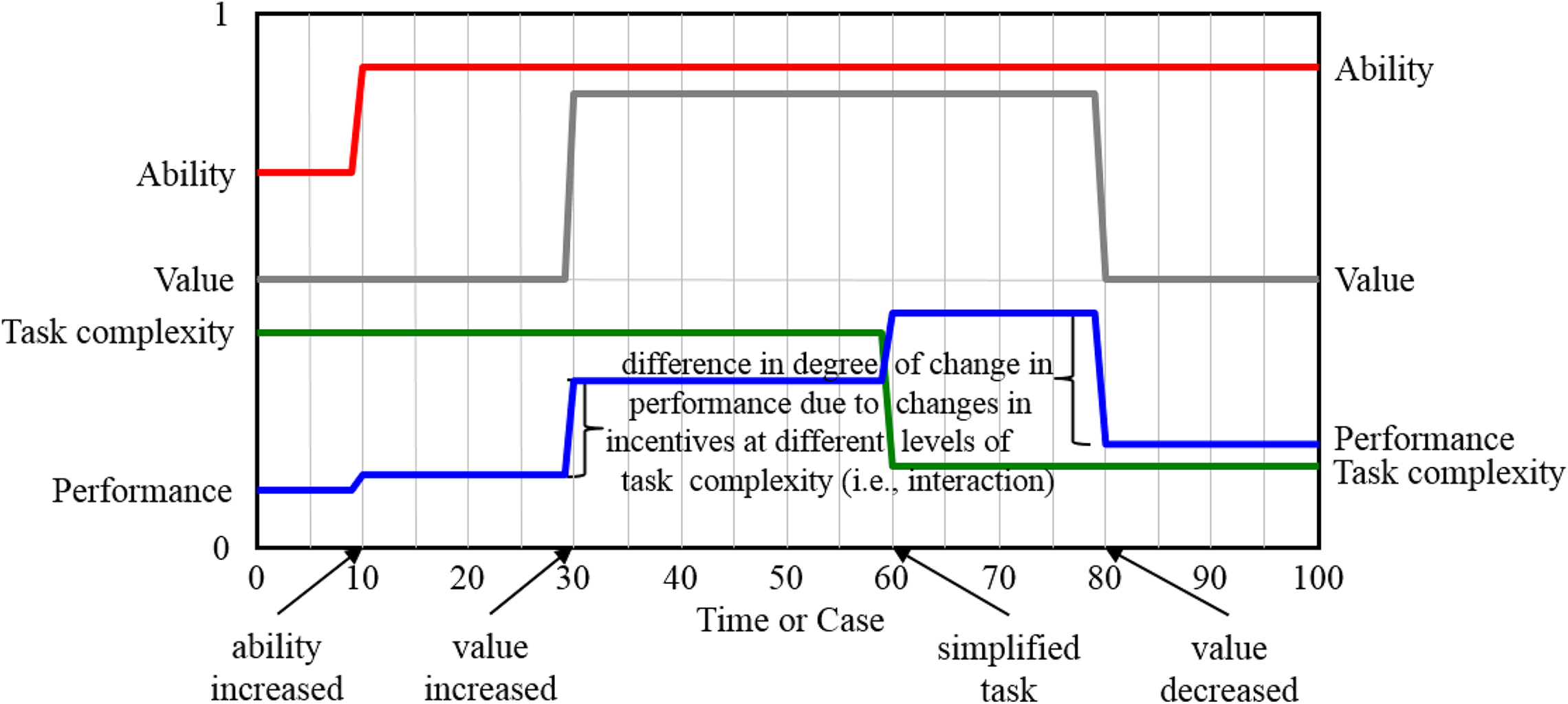
Static model results.
The results of the simulation of the static model confirmed that it is coherent and a reasonable representation of the IMWM core (i.e., that it is internally valid). For example, Figure 4 shows that changes in the exogenous variables were related to performance as predicted by the nonformal model and found empirically (Locke & Latham, 1990). That is, performance improved when ability improved, value increased, and the task became less complex. Moreover, the moderators acted as predicted. This can be seen in the degree of change to performance when value first rises and then falls by the same amount (see brackets in Figure 4). Despite the equal change in value, the effect of the change on performance is greater when value returns to its original level compared to when it first changed. This is because task complexity was less the second time value changed, increasing the effect of the change.
We also confirmed that the key manipulations used to develop goal theory produced the effects expected. To illustrate these effects, we present the effect of changes in goal value (i.e., increasing at Time 30 and decreasing at Time 80) as one might see in a repeated-measures study using an ABA design (see Figure 5). The y-axis is personal goal level. Each line represents an individual in one of four goal conditions (i.e., no goal, easy goal, moderate goal, and difficult goal). Note the no goal condition represented a low goal specificity condition and the three assigned goal conditions were nested within the high goal specificity condition.
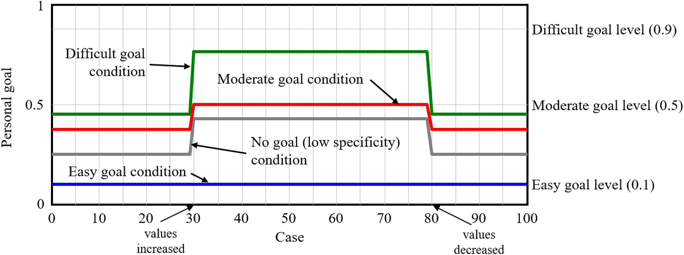
Personal goals for three assigned goal conditions (i.e., easy, moderate, and difficult) and a no goal (i.e., low specificity) condition.
In particular, the figure shows that when assigned an easy goal (i.e., assigned goal level was set to 0.1, meaning that only 10% of the population would not achieve this level of performance), the assigned goal was accepted regardless of the level of value. In contrast, the figure shows that for those in the moderate, difficult, and no goal conditions, value positively related to personal goal. In the case of the individual in the assigned moderate goal condition, the increase in value caused the personal goal to go to the moderate goal level (i.e., 0.5), representing the notion that the goal was accepted. However, in the difficult goal condition, personal goal increased with value but not to the assigned goal level of 0.9 (i.e., level of performance that 90% of the workforce could not reach). Rather, the personal goal was a function of motivational force (i.e., Value × Self-Efficacy) for all the times, including both the A and B phases of the experiment for the individuals in the no goal and difficulty conditions.
Theoretical Implications of the Static Model
Two interesting theoretical implications emerge from these simulations. First, they showed that for more difficult goals (i.e., the moderate and difficult assigned goal conditions), the effect of assigned goal difficulty manipulation on performance observed in goal-setting studies (Locke & Latham, 1990) has to do with its effect on self-efficacy. This can be seen by comparing the effects of no goal, moderate goal, and difficult goal conditions on goal level. In particular, when value was relatively low, the personal goal was not at the assigned goal level. Rather, it was at the level of the motivational force (i.e., the product of self-efficacy and value). Further, the positive difference in the personal goals for those in the moderate compared to the difficult assigned goal conditions is exclusively because of the assigned goal’s influence on self-efficacy.
The other interesting finding highlighted by the simulations of the model is that except for the positive indirect effect of goal difficulty on self-efficacy, assigned goals only constrain the level of personal goals. This can be seen in Figure 5 with regards to the easy and moderate goal conditions. For the easy goal, the personal goal never exceeds the assigned goal level regardless of the increase in value. In the moderate goal condition, the personal goal takes on the assigned goal level (i.e., 0.5) despite a motivational force that is greater than 0.5. To be sure, the individual in the moderate goal condition shows a higher personal goal than the no goal condition individual because the assigned moderate goal increased self-efficacy. However, if self-efficacy or value already started a little higher, the individual in the no goal condition would have adopted a higher goal from the beginning or once value increased. Thus, this model suggests that one either assign no goal or make sure the goal is very high, particularly if the effect of an assigned goal on self-efficacy is small (e.g., weight is small). Indeed, Locke (1997) had already reached this conclusion based on empirical work, but it will not be clear until we render the dynamic model how important this notion is. In particular, the empirical literature finds that the effect of an assigned goal on self-efficacy is negligible when the individual has experience with the task (Earley & Lituchy, 1991). It is also important to note that although personal goal is constrained by the assigned goal, changes in ability, value, or task complexity still affect performance in the model because these exogenous variables affect endogenous variables beyond personal goal.
In sum, our attempt to operationalize the static IMWM proved largely successful. The effects of variables, including the constraining effects of less than difficult goals, are consistent with those found in the goal literature (Locke et al., 1981). However, some effects described in the literature were not reflected in the computational model. For example, when difficult goals are assigned, the goal choice mechanism gives no boost to the level of personal goal beyond what comes via the boost to self-efficacy. Further, the acceptance of a goal does not increase goal commitment, as is often assumed in the escalation of commitment literature (Sleesman, Conlon, McNamara, & Miles, 2012). This means that either (a) changes to the functions are needed, (b) a closer scrutiny of the empirical literature and the conclusions drawn from it is needed, or (c) a modified architecture/theory is needed. Relevant to the last option, a serious limitation to the modeling done thus far stems from the static nature of the IMWM. Given the inherent dynamic nature of motivational processes (Diefendorff & Chandler, 2011; Schmidt, Beck, & Gillespie, 2012), this lack of consideration of dynamic processes may undermine the value of any motivation model. To address this shortcoming, we investigate whether the IMWM can be extended to a dynamic model or, if not, what might be done to make it viable.
Building and Evaluating Dynamic IMWMs
Keeping to the core components of the IMWM, we focused on the one explicitly dynamic element in the IMWM, which is the feedback loop from performance to self-efficacy (Locke, 1997). Specifically, we added performance as an input in the self-efficacy function. This link reflects Bandura’s (1997) premise that self-efficacy’s chief cause is past performance, which has been robustly supported by research (Sitzmann & Yeo, 2013). However, because we now present the passage of time, we also changed other aspects of the model. For instance, to reflect Earley and Lituchy’s (1991) finding that assigned goal difficulty only influences self-efficacy when one is unfamiliar with the task, the weight of the assigned goal difficulty effect should fade over time. Thus, to represent this reducing goal assignment effect, we divided the previously used weight by one plus time, where the time variable was weighted by fade to test the model under different rates of a fading assigned goal effect (i.e., 0.5 / [1 + Fade × Time]). Specifically, because time increases over the course of simulations of the dynamic model, this function results in assigned goal difficulty having a smaller effect on self-efficacy over time. We initially set fade to 1. Meanwhile, the 1 in the function starts the weight out at the 0.5 level and prevents the denominator from being 0 at the beginning of a simulation (i.e., when time = 0). The dashed boxes and arrows pointing at weight in Figure 6 reflect this initial dynamic model. The function can be found in the third column in Table 1.
Dynamic integrative model of work motivation (IMWM).
Another issue for a dynamic model was the role of goal commitment. Recall that goal commitment is a function of the same factors and has the same functional form as goal choice. Indeed, goal choice represents the process for goal acceptance, and the distinction Locke and Latham (1990) make between goal acceptance and goal commitment is a dynamic one. That is, goal acceptance refers to the process by which a personal goal is adopted, and goal commitment refers to the process by which a personal goal is retained. Yet the processes are assumed identical. In the dynamic model, the goal choice function is continually operating and thus represents the process by which the personal goal is accepted as well as retained. This makes the goal commitment construct redundant in a dynamic model and thus could be removed. Given our larger purpose of illustrating the value of computationally modeling existing theories that are often static, this revision shows how a dynamic model can increase the parsimony of a theory. 8
Removing goal commitment also simplified the goal mechanism (i.e., effort) function. Yet moving to a dynamic model put into play a better effort function. In particular, the general notion in goal theories is that performance is regulated via a negative feedback function (e.g., Austin & Vancouver, 1996; Bandura, 1986; Locke & Latham, 1990). The negative feedback function is analogous to a cruise control mechanism that regulates speed. That is, some level of force (e.g., engine torque) is applied to maintain a desired speed by increasing or decreasing the force when the speed is slower or faster than desired, respectively. In this example, force is a level variable (Forrester, 1968; Vancouver, Weinhardt, et al., 2010). Level variables have memory or inertia (Cronin & Vancouver, 2019). That is, they retain their values (or levels) over time unless moved one way or the other (Powers, 1978). In platforms that represent time as continuous, this property is represented using an integration function (i.e., ∫ [x] dt). In the case of the goal mechanism function, the effort applied to obtain some desired level of performance, represented by one’s personal goal, would change based on the difference between the goal and performance. That is, effort changes as a function of the difference between personal goal and performance (i.e., ∫ [personal goal – performance] dt). Thus, performance now affects effort as well as being affected by effort (see dashed arrow from performance to effort in Figure 6).
However, recall that the goal mechanism function also includes the constructs of feedback and possibly self-efficacy. Research has shown that feedback can moderate the effect of self-efficacy on effort and performance such that the effect is positive when feedback is present but negative when feedback is low or ambiguous (e.g., Schmidt & DeShon, 2010). Vancouver and Purl (2017) explain that the positive effect is via a goal choice mechanism similar to the one presented here. Meanwhile, the negative effect occurs when and to the degree feedback is ambiguous via a process of positively biasing the performance perception used in the effort function. This logic and the complete revised effort function is represented in Table 1. 9
Building Different Dynamic Functions for Self-Efficacy
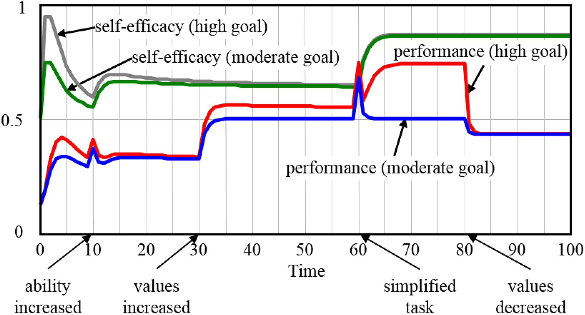
As mentioned, the IMWM did not specify the concrete form of the reciprocal relationship between self-efficacy and performance. Therefore, in the current study, we evaluated three possible dynamic functions that link performance back to self-efficacy and closes the feedback loop. In doing so, self-efficacy is also modeled as a level variable because self-efficacy is a belief and beliefs are level variables (Vancouver et al., 2014). That is, one retains a belief unless information causes one to reconsider the belief (e.g., after tasting a particularly good apple, one might adjust upward one’s belief in the tastiness of apples, or after experiencing poor job performance, one might adjust downward one’s self-efficacy regarding one’s capability). As noted previously, modeling continuous change in level variables requires an integration function with some initial level of the level variable plus the inputs that move the level variable one way or the other (Vancouver, Weinhardt, et al., 2010). The first such dynamic function we used to link performance to self-efficacy is the following positive relation function:
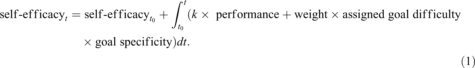
The equation can be read as follows: Self-efficacy at time t is a function of initial self-efficacy at t 0 and performance plus the assigned goal difficulty effect integrated with respect to time. Our default value for initial self-efficacy, t 0, is represented in the personality variable and set to 0.5. The term k represents performance’s feedback effect on self-efficacy. It was also set to 0.5, though examined at different levels (e.g., setting it to 0 removes the feedback effect). Specific to the relationship between performance and self-efficacy, this equation means that at a given moment, self-efficacy is a function of the cumulating, positive, linear effect of past performance between t 0 and t. This functional form is consistent with both the theoretical notion that performance is positively related to self-efficacy (Bandura, 1997) and the majority of empirical findings that supported the positive linear relationship between the two variables (Sitzmann & Yeo, 2013). An issue with it, though, is that it means that when individuals achieve any positive performance on a task, their task-specific self-efficacy improves.
The second dynamic function that we examined used change in performance rather than performance itself as an input to self-efficacy. The mathematical form of this function is:
According to this function, a positive change in performance increases self-efficacy, and a negative change decreases self-efficacy. To determine change in performance, past performance was subtracted from current performance. This required an additional initial performance value. Given that we stipulate that the beginning of the simulation represents the initial experience with the task, this initial performance value would best be considered imagined or estimated. One place to obtain such an estimate is one’s self-efficacy, which is initially a function of personality. Thus, we used personality to obtain the initial past performance value.
The effect of changing performance was determined by the same parameter, k, described previously, though here it represents the degree of impact that changing performance had on self-efficacy. Conceptually, this dynamic function represents the idea that self-efficacy only changes if performance changes and the direction of the change of self-efficacy is consistent with the direction in the change in performance (Elicker et al., 2010). Accordingly, this function can explain the prediction that the same level of performance may generate different levels of self-efficacy because the changes (i.e., performance improvements/decline) may be different (Carver & Scheier, 1998; Lord, Diefendorff, Schmidt, & Hall, 2010).
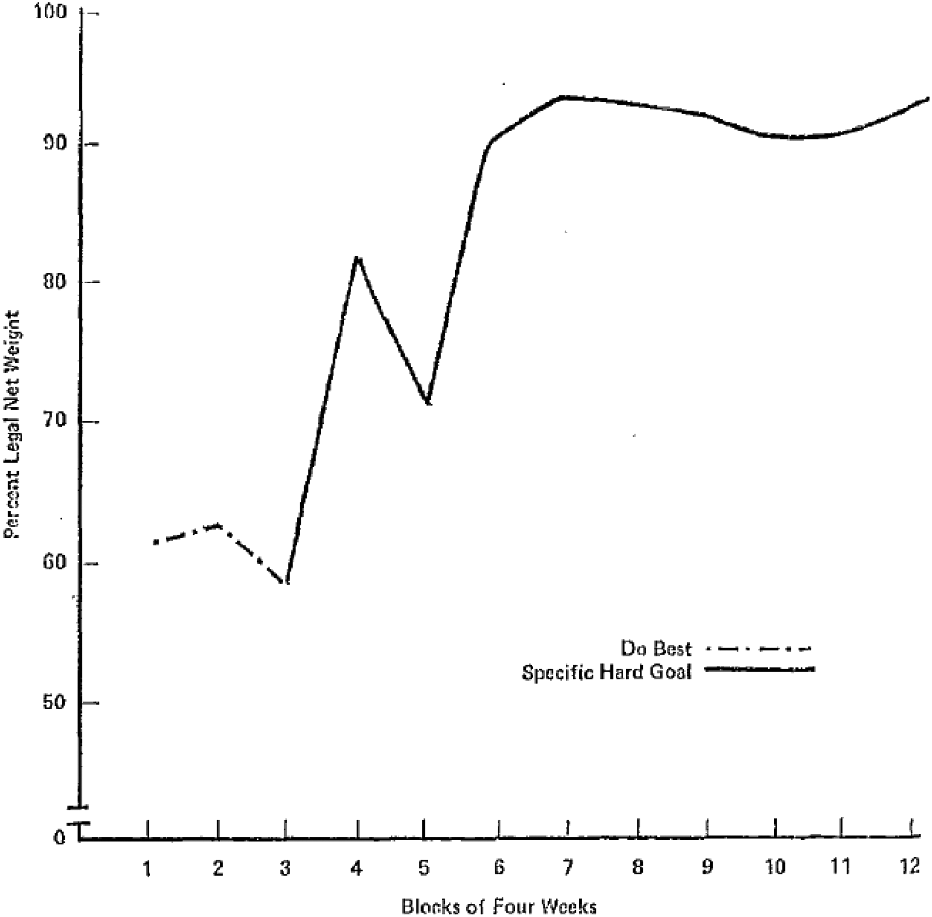
The third dynamic function we examined is a calibration function where self-efficacy adjusts to reflect performance. Such functions are common in learning models (Anderson, 1995), where beliefs are updated based on a fraction of the difference between the current level of the belief and new information (Vancouver et al., 2014). The new information is observed performance given effort applied. Specifically, by dividing performance by effort, the individual can deduce capability. The mathematic function is:
Theoretically, this calibration function represents the notion that individuals update existing self-efficacy beliefs when information (e.g., performance given effort) suggests the existing beliefs might be incorrect. However, a k parameter, which is usually less than 1, suggests that individuals are not completely swayed by the new information they receive; rather, they compare the new information with their existing beliefs and change their beliefs by only a fraction of the discrepancy. Via this process, self-efficacy beliefs align with capability over time at a rate determined by k. The calibration process is consistent with arguments Bandura (1997) makes regarding self-efficacy as well as research on self-efficacy and performance effects over time (e.g., Shea & Howell, 2000; Sitzmann & Yeo, 2013). An important feature of this function is that it guarantees that self-efficacy is on the same scale as capability.
In sum, the aforementioned three dynamic functions represent three theoretical mechanisms that have been commonly used to describe and conceptualize the effect of performance on self-efficacy in the research of work motivation. In the following, we evaluate how theoretically coherent they are by simulating computational models that incorporate each one of them.
Evaluating the Dynamic Models
Evaluating the Dynamic Model Based on the Positive Relation Function
Simulating the positive relation function (i.e., Equation 1) in the dynamic model resulted in runaway trajectories and a floating-point error due to generating a very large number. Though this might be consistent with the positive spiral for self-efficacy and performance that Lindsley, Brass, and Thomas (1995) discuss, the behavior observed using this model occurred regardless of the individual or contextual differences we represent in the model. The only exception was when value was set to 0. That is, it would represent a world with either completely inert employees or highly motivated employees whose motivation and performance with respect to a goal continually improved at an increasing pace over time (cf. Lindsley et al., 1995). This seems to indicate that the dynamic model based on the positive relation function is unlikely to be a valid representation of reality.
However, before abandoning the positive relation model, we attempted to solve the increasing rate of improvement problem that occurred in the simulation by adding a performance limit. Specifically, Locke (1997) noted that goal difficulty’s positive effect on performance is limited by ability. Thus, we revised the performance equation such that it could not exceed the individuals’ ability level (we retained ability as a moderator as well). When this model was simulated, self-efficacy and all the variables affected directly or indirectly by self-efficacy continued to rise, though no longer exponentially once the performance limit was reached. At that point, performance no longer changed, but all other variables rose at a steady rate (i.e., the rate of ability level). Thus, the model represented a world where self-efficacy (and effort, etc.) would increase constantly once it began such a trajectory. This behavior does not appear to be consistent with reality as we know that self-efficacy can fluctuate in nonmonotonic ways over time (e.g., Vancouver, Thompson, & Williams, 2001). Thus, we moved on to evaluate the change function.
Evaluating the Dynamic Model Based on the Change Function
The change function (i.e., Equation 2) represented the notion that self-efficacy changes when performance changes. Simulations of this model showed that performance and self-efficacy increased and decreased as expected given changes to the exogenous variables. A minor issue was that self-efficacy levels often rose above 1. More problematic was the effect of differences in initial estimated performance. Specifically, when initial estimated performance was higher than observed performance, self-efficacy dropped because of the apparent drop in performance. This drop in self-efficacy only reduced performance more, leading to a further reduction of self-efficacy. This negative spiral continued until self-efficacy reached 0. Likewise, when goal specificity was low, an initial improvement in performance from initial estimated performance would raise self-efficacy, which would raise performance until one’s ability level was reached. These processes produced a bimodal distribution of performance. Thus, like the positive relation model, the simulation results yielded from the change in performance model seem to deviate from reality. More generally, this sensitivity to an initial setting of the model is not ideal for a computational model (Davis et al., 2007).
Evaluating the Dynamic Model Based on the Calibration Function
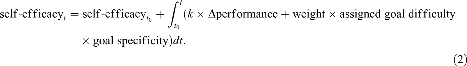
The last dynamic self-efficacy function examined was based on Equation 3. As before, we tested the revised model by assessing the effects of two assigned goal levels: a moderate (0.5) and high (0.9) goal. We also included the changes to ability, value, and task complexity used when examining the static model. The results of simulating the calibration model are shown in Figure 7. In this case, the model is dynamic, which means the figure provides the trajectories on the variables across time. Specifically, Figure 7 represents the trajectories for self-efficacy and performance for an individual assigned a moderate goal and a different individual assigned a difficult goal.
Performance and self-efficacy in two assigned goal conditions.
Focusing first on self-efficacy, the results show that although the level fluctuates some across time, the two individuals’ beliefs merge and stay together across the rest of the simulation. This finding is expected given the only source of a difference is the assigned goal difficulty effect. However, the assigned goal difficulty effect had decreasing influence over time (Earley & Lituchy, 1991). It caused self-efficacy to increase from its initial 0.5; however, both individuals quickly begin to calibrate their beliefs to 0.49, which was their capability (i.e., ability × [1 – task complexity]) for the first 10 time steps of the model. At Time 10, ability increases to 0.9 (e.g., the individuals received training), and thus capability increases to 0.63. Both trajectories approach this value until task complexity drops to 0.05 at Time 60 (e.g., a job design change simplified the task). At that point, both trajectories increase to just above the 0.86 value that represents both individual’s increased capability.
Regarding performance, Figure 7 shows performance initially increases and the increase is higher for the individual in the high goal condition. The increase is because effort increases from its initial value based on the difference between personal goal and performance. That is, it represents a person seeking a level of effort that gets performance to personal goal level. The downward “correction” is because the modeled individual overshoots the needed amount of effort. That is, the model represents the idea that individuals are seeking an equilibrium for effort to obtain the level of performance represented by the goal level. Moreover, the increase in self-efficacy caused by the assigned goal is higher for the individual in the high goal condition, which bumps up the goal more for that individual. Meanwhile, self-efficacy is also calibrating to capacity, which takes some time. These forces have not quite reached equilibrium when the “training” increases both individuals’ ability at Time 10. In our opinion, this finding illustrates an opportunity to empirically challenge the dynamic model of IMWM. That is, an empirical study might be constructed that can examine the dynamics represented in these first 10 time steps. Nevertheless, prior to conducting such a study, it is important to consider that ability might improve over time due to experience. This could be operationalized into the model to get a range of predictions. The key would be to see whether the observations from empirical data were outside that range.
Another potentially interesting effect is observed at Time 10, when performance spikes. This occurs again at Time 60. These are the two times that the performance moderators (i.e., ability and task complexity) are changed. In the model, the uptick occurs because the multipliers take on a higher value (i.e., capability increases), and the drop occurs because the goal mechanism needs a time step to adjust effort to the lower level needed to reach the desired level of performance (i.e., the personal goal). That is, it takes a time step for the feedback to reach the goal mechanism, and thus the mechanism is putting out the same level of effort at the point before the capability had increased. In this case, because we had no k weight slowing the calibration of effort, the correction takes only one time step. This might be an interesting observable phenomenon revealed by the model. However, it can also be an artifact of the way the dynamics are represented. Specifically, if capability changes slowly or the delay in feedback is short (i.e., occurs within the time step represented here), this model would not reveal these spikes (see Vancouver & Scherbaum, 2008). That is, the spikes are not because of the functional forms (i.e., the theory) but rather, granularity of the time step intervals represented. Thus, the conditions of the model would have to be similar in terms of the dynamics of reality if one wanted to test the model based on this observation.
Finally, like the static model, the performance trajectories reveal that the goal level effect occurs via the lower effort applied by the individual in the moderate goal condition as compared to the high goal condition once motivational force (i.e., self-efficacy × value) was high enough for the individual to adopt that assigned goal level. Meanwhile, the individual in the high goal condition did not adopt a moderate goal level—because it was not offered—and thus applied enough effort to reach higher levels of performance until the value level was returned to its original level at Time 80. This last effect confirms that goal commitment is not needed in this dynamic model. That is, once value dropped, both individuals abandoned the goal levels they had adopted. Thus, this finding shows that the dynamic model can reproduce the key finding of the goal difficulty effect from goal-setting theory (Locke & Latham, 2002). However, it also shows that if the model is correct, goal setting as an intervention only “works” because one might get lower performance from those given goals lower than their own motivational force.
We should also point out that the interpretations made previously are difficult to derive from simply reflecting on the trajectories. We know this because our initial thoughts regarding the observed trajectories were incorrect though we had built the model that made them. It was only after examining functions for the constructs and the values these functions created across the time steps that we realized what was driving the trajectories. Thus, the model and its simulations provide the information needed to diagnose the process responsible for the trajectories.
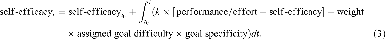
Testing Calibration Function Model Against a Longitudinal Empirical Referent
As a final check of the dynamic IMWM model, we represented the conditions of a longitudinal study with time-series data used to examine goal-setting effects in the field (Latham & Baldes, 1975). Time-series data are much more diagnostic regarding dynamic models because several alterative models might produce a set of relationships among variables but fewer models are likely to create a set of trajectories. Latham and Baldes (1975) examined the load, relative to maximum legal load, of logging trucks over a 48-month period. Baseline data indicated that the 36 trucks in the study were loaded at about 60% capability, on average. After the third month, a difficult goal of 94% was assigned to the truck drivers. Figure 8 shows the average percent legal net weight of the trucks for each 4-week block reported in Latham and Baldes. The test for the model is to see if it can produce the trajectory illustrated in the figure, except for the Month 5 downward dip, which Latham and Baldes attributed to the drivers’ testing the claim that no punishment would befall those failing to reach the goal and thus involves a process beyond that considered in the IMWM.
Percent legal net weight of 36 logging trucks.
To represent the Latham and Baldes (1975) study in the computational model, we (a) set the time steps to one week, (b) set the assigned goal to 0.94, and (e) added a STEP function to the goal specificity variable that switched its value from 0 (i.e., the no goal condition) to 1 (i.e., the assigned goal condition) at Time 30. The time step was chosen to provide time for any initial dynamics in the model to settle prior to the baseline period. We set task complexity to 0.2, given the task determining the load on the trucks was likely relatively easy. We set ability to 1 because in this case, performance reflected the percent legal net weight and all the truckers would presumably be able to reach the limit. Finally, we set value to 0.5, though this parameter, along with personality, k (i.e., the weight that determined the rate at which self-efficacy was updated), task complexity, and ability were parameters that we varied to fit the trajectory produced by the model with the trajectory illustrated in Figure 8.
The initial sensitivity analysis involved varying the personality parameter between 0 and 1 at increments of 0.1. As expected, personality had a substantial initial effect on self-efficacy, but that effect was gone by Week 10 in the simulation regardless of the personality value used. This confirmed that initial dynamics would settle for the baseline observations. Next, we attempted to get the baseline level of performance (i.e., the level of performance once the initial dynamics had settled and prior to the introduction of the assigned goal) to about 0.6. Given the ability and task complexity levels noted previously, this was achieved by setting value at 0.75. Unfortunately, given the parameters and structure of the model, the effect of the assigned goal on performance upon its introduction at Week 30 was negligible.
To get a substantial effect, we reduced the fade parameter to 0.05, which translated to a weight for the assigned goal effect of 0.2 and thus the effect of the assigned goal of 0.188 on self-efficacy at Time 30. We also had to set k to 0.3. With these parameter values, we obtained the trajectory labeled via self-efficacy shown in Figure 9. Three important points need to be made about this trajectory. First, the assigned goal effect bumped self-efficacy up to a maximum of 1.34 at about Week 36. This seems like an unrealistically high number, but if the scale is net weight relative to legal limit, one might believe they are capable of achieving 34% above that legal limit after given the assigned goal of 94%. However, even then, performance began to decline at Week 53 in the simulation. Eventually, it returned to baseline (not shown).
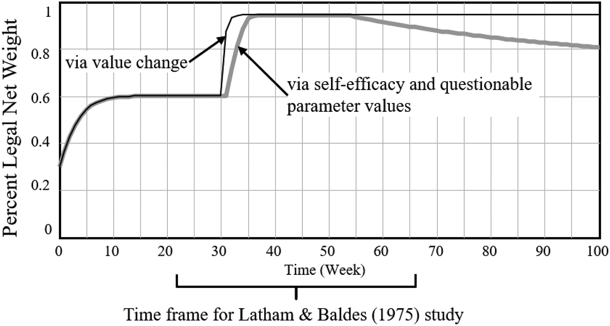
Sample trajectories from dynamic integrative model of work motivation (IMWM).
The aforementioned results of the simulation created several theoretical and practical challenges for the IMWM. First, it requires the notion that an assigned goal substantially affects self-efficacy despite what was potentially years of experience with the task. Moreover, the level that self-efficacy needed to accept the assigned goal was well above the level of performance previously experienced as well as the level of performance required to achieve the goal. Indeed, the assigned goal effect had to be strong enough to counter the calibration process, which it could only do if the calibration rate, k, was low. Moreover, the assigned goal effect had to continue well past the point of the goal assignment, and even then, it eventually dissipated enough for the slowed calibration effect to begin lowering self-efficacy. Because of this, self-efficacy and thus performance eventually return to the equilibrium represented by the pre-assigned goal baseline. In other words, if this theory accurately represents the processes involved in determining the “practical value” of goal setting (Locke & Latham, 2002), one can expect that practical value will not last. The fact that it took a long time for this return to baseline in the simulation is likely due to the unrealistically low parameters for the fade and k parameters needed to achieve the trajectory observed by Latham and Baldes (1975). Indeed, research on the dynamics of self-efficacy, including the research Locke (1997) cites to suggest the model generalizes to a dynamic version (i.e., Mone, 1994), does not seem to support this self-efficacy–based interpretation of the Latham and Baldes data.
Given the aforementioned issues, we sought to consider an alternative model that might account for the Latham and Baldes (1975) data. For example, one might speculate that loggers’ personal goals were largely determined by a social norm and the assigned goal manipulation triggered a positive feedback loop by creating a competition among the loggers that resulted in a change in the social norm. Indeed, Latham and Baldes noted in their discussion that “anecdotal information suggests that goal setting did lead to informal competition among drivers” (p. 124). Thus, the loggers might have always believed that they could perform at a higher level (i.e., self-efficacy was high), but they did not adopt a goal that was consistent with the belief because, for instance, there was little value in it (e.g., high loads increased the danger, which countered positive value to higher loads). Latham and Baldes also suggested that the assigned goal might have provided drivers with “a sense of achievement, recognition, and commitment” (p. 124), which might be interpreted as an increase in value. Finally, it might be that the loggers also realized that by loading their trucks at 94%, particularly if all of them did that, they could make fewer trips and that increased the value of performance. That said, we should note that Mento, Locke, and Klein (1992) found a negative relationship between goal level assigned and valence (i.e., anticipated satisfaction across several levels of performance), but anticipated satisfaction may well be different than the value of performance to the individual. Indeed, incentive systems can vary substantially (e.g., bonus for reaching a goal, piece rate unrelated to goal, or piece rate that drops for levels of performance above the goal), and these variations would likely affect motivational force via different functional forms (Pritchard, Jones, Roth, Stuebing, & Ekeberg, 1988). In other words, refinements of the goal choice mechanism function (i.e., the one that determines personal goal) and/or the value function are likely needed.
As a start, we wanted to determine if the Latham and Baldes (1975) findings could be explained by an assigned goal triggering an increase in value. We assessed this by adding an assigned goal effect on value (i.e., assigned goal level times weight of 0.5). We also removed the assigned goal effect on self-efficacy. The via value change trajectory in Figure 9 shows the results of this revised model. As can be seen, this trajectory presents a quick and long-lasting effect on performance. Thus, assigned goals may have triggered, at least in this case, an increase in value that leads to the performance effect. It is this final model that is represented in Vensim and Matlab code in Appendices A and B, respectively.
Discussion
Several recent papers have lamented the state of theory in the field (e.g., J. R. Edwards, 2010; Leavitt et al., 2010; Mathieu, 2016). For example, Antonakis (2017) criticized the tendency to seek new theory and the lack of rigor in both new and old theories. Likewise, J. R. Edwards and Berry (2010) advocated more precision in theories via, among other means, the specification of the functional form of the relationships described in a theory. To help address this issue, we suggest the use of computational modeling (Weinhardt & Vancouver, 2012). To illustrate the process and its usefulness, we created a computational model of Locke’s (1997) IMWM. The IMWM includes classic theories of motivation, including expectancy (Vroom, 1964), social cognitive (Bandura, 1986), and goal theories (Locke & Latham, 1990), among others (Locke 1997). Moreover, the IMWM was presented as a static theory with dynamic ambitions (Locke & Latham, 2004). Thus, we rendered both a static and dynamic version. This allowed us to demonstrate that dynamics can add substantial, difficult to predict complications to theoretical propositions that computational modeling can help reveal. In the following sections, we discuss the implications of the model for the IMWM as well as the implications of computational modeling as a method for vetting old theories and encouraging research to assess those theories.
Theoretical Implications of the Computational Models and Simulations of the IMWM
The most immediately noticeable implication that arose during the process of building a computational model of the IMWM was the lack of specifications of functional forms for key constructs. Rather, as is typical of theories in the field, the factors that influence a process and the sign of the effects are specified but often little more (J. R. Edwards & Berry, 2010). For example, one can find several descriptions of goal choice processes that suggest that value, or some synonym for it (e.g., valence), and self-efficacy, or some synonym for it (e.g., expectancy), positively predict personal goal, but how these inputs are combined (e.g., additively or multiplicatively) to determine a specific value for personal goal is unclear (cf. Gee, Neal, and Vancouver, 2017). Moreover, when an externally presented goal becomes an input (i.e., an assigned goal), the functional form is even more ambiguous. The functional form we developed seemed to reflect the nonformal descriptions presented and theories evoked (e.g., expectancy theory), but it may not. Indeed, more important than creating functions that represent what some set of theorists meant, the larger question is whether it reflects the actual process. The computational modeling exercise highlights (a) which functions are most critical, (b) what we think we know about them, and (c) what that thinking can mean. It appears that we generally know less than we need to know to create valid, workable functions, pointing us to a direction for future research.
As a specific example of a functional form that was ambiguous was the one related to self-efficacy in the dynamic model. In that case, we illustrated the role computational modeling can play in researching the possible forms. Specifically, we evaluated three potential functional forms computationally, eliminating two of them based on the results of simulations. We should point out that typical computational modeling papers are unlikely to write up this model development process. That is, modelers may explore alternative functions by creating and simulating them because predicting their effects can be difficult without the support of the modeling platform (Davis et al., 2007), but they will tend to save readers from the burden of this development and testing process (Hintzman, 1990). We included it here to show what one might do while translating an existing nonformal theory to a computational one.
Another advantage the translation process revealed, particularly as we transitioned from the static to the dynamic model, was the increased ability to represent nonformal or other descriptions from the nonformal theory into the formal rendition. For example, Bandura (1986) uses control theory’s negative feedback loop, what he calls reactive control, as a key mechanism that translates personal goals into effort and behavior. Yet such a description cannot be rendered in a static model. Thus, it was only at that point that we could create a more internally valid representation of the descriptions that informed the IMWM. The transition also motivated the addition of the ability ceiling to performance (Locke, 1997). Finally, the transition process allowed for a more parsimonious theory by allowing the removal of goal commitment as a construct given its process was captured in the goal choice mechanism.
In addition to the functional form issue is the issue of how the constellations of constructs and causal processes described in a theory play out over time. Nonformal theories often describe, either implicitly or explicitly, positive feedback loops among the constructs in the theory. We would not argue that such loops are uncommon but that they are unstable (Forrester, 1968). Some dampening, negative feedback process is generally involved that provides stability to the system. Rendering these processes computationally can reveal, in the case of unchecked positive loops, an implausible theory or in the case of negative feedback loops, the likely short-term effects of interventions. In terms of the IMWM, the first two dynamic functions for self-efficacy demonstrated two variations of the positive feedback loop problem, and the third dynamic function revealed the tendency to return to equilibrium reality common to systems with negative feedback loops. Indeed, for such systems, the issue is figuring out how to change the system such that it has a new equilibrium of the sort desired. The difficulty practitioners have in making long-term desired changes often stems from the incomplete understanding of the dynamics involved (Forrester, 1968). In the present case, our model of the IMWM revealed that changes to some exogenous variables (e.g., ability, task complexity) produced stable change, whereas changes to other variables (e.g., specifying a difficult goal) did not.
General Implications of Computational Modeling
Besides raising issues regarding the IMWM, the modeling effort provided here highlighted the value and use of computational modeling more generally. For example, when building and evaluating computational models, Davis et al. (2007) advocated “experimenting” with them to assess and help develop theories. Much of this uses sensitivity analysis, which involves examining the model under various levels of the exogenous variables. As Davis et al. note, much of this analysis is not reported in write-ups of computational models, which we largely honored. An exception was our explicit tests of the ability of the models to reproduce key findings from the goal literature. Specifically, by using different values within or across simulations, we “manipulated” five exogenous variables (goal specificity, assigned goal difficulty, ability, value, and task complexity) to evaluate the validity of the static and dynamic renderings of the IMWM. The first thing we confirmed was that the static model produced results that were consistent for empirical research for all the exogenous variables examined. This included the finding that the goal difficulty effect was largely a function of easier goals reducing motivation rather than higher goals increasing motivation (Locke, 1997). The only possible addition to motivation caused by goal difficulty was the bounce in self-efficacy that a difficult goal might provide (Earley & Lituchy, 1991). Unfortunately, Earley and Lituchy (1991) also found that this bounce is relatively short-lived, and our dynamic model showed that unless the bounce lasted a long time, the theory predicts that the effect of assigning a difficult goal is not likely to change performance much or for long. To be sure, parameter values could be used to create a greater and longer lasting effect, but these values seemed difficult to defend psychologically and empirically. What our modeling seems to reveal is that based on the IMWM, a nonspecific do your best goal is most likely to get the best performance in the end because it removes the risk that the assigned goal level is below the level the individual would settle on after experiencing the task.
The difficulty the dynamic model had reproducing the Latham and Baldes (1975) findings motivated an alternative model where the assigned goal affected the value of the task rather than self-efficacy. This model produced the effect, and it was long-lasting. That said, we are not prepared to endorse our revised model as a new theory of goal setting’s effects. One source of reticence is that it was motivated by a single study that was not directly designed to test it or competing theories. More important, we merely verbally described possible reasons for an assigned goal effect on value (e.g., a social competition process). That is, we represented the presumed results of some process but not the process itself. We suspect that better (i.e., more accurate in terms of describing the results of the human information processing system) functional forms for value and the goal choice mechanism should be explored both computationally and empirically. As models with finer grained analysis have shown regarding the goal mechanism (e.g., Ballard, Yeo, Loft, Vancouver, & Neal, 2016; Vancouver et al., 2014; Vancouver & Purl, 2017; Vancouver, Weinhardt, et al., 2010), the processes are likely complicated, and thus the simple functional forms might not capture the results of these processes well. Indeed, a major limitation of the IMWM is its single-goal boundary condition. The operations represented in these computational models hinge on properties of the competing goals. Thus, the failure of the dynamic IMWM to account for the empirical referent might have to do with its myopic focus on the single-goal context.
Computational models can facilitate theory testing not only because they provide a test of the theory’s logic but also because they can inform measurement and empirical testing. For example, Atkinson, Bongort, and Price (1977) used a computational model of the dynamics of motivation to reveal the limitations of Cronbach’s alpha for evaluating the reliability of measures of needs derived from the Thematic Apperception Test (TAT). This computational model inspired subsequent researchers to develop and test item response theory (IRT) models for deriving construct scores from TAT methods (Tuerlinckx, De Boeck, & Lens, 2002) as well as a process model that could explain the inconsistency between the metrics of reliability (Lang, 2014). Likewise, Vancouver (2009) discussed the use of computational models to measure person properties revealed as the individual interacts with the environment over time.
In terms of empirical testing, computational models can be used to develop predictions for trajectories of variables over time or associations among variables that one might observe empirically via sensitivity analysis based on simulating two or three levels of a variable as done here (e.g., see Figure 7) or via more comprehensive simulations using Monte Carlo methods to populate parameter or exogenous variable values from specified distributions (e.g., Vancouver et al., 2016). They can also show the limitations of traditional empirical designs used to test theories. For example, Vancouver, Tamanini, et al. (2010) used two computational models to reveal why existing studies used to assess a key theory of information seeking were inadequate. On a more positive note, Vancouver and Scherbaum (2008) created computational models of competing theories of self-regulation and used them to develop an empirical study that pitted the theories. Computational models can also be fit to time-series data from single cases (e.g., Vancouver, Weinhardt, et al., 2010) or a set of cases simultaneously (Ballard, Vancouver, & Neal, 2018). Of course, the caveats associated with data fitting that apply to statistical modeling also apply to computational modeling. For example, the more parameters and the less constrained they are, the more easily a model will fit and thus the less diagnostic the test and the less predictive the theory (Myung, 2000; Roberts & Pashler, 2000). A weakness of our empirical referent is that we only had the average trajectory. A weakness of the IMWM computational model is that we could set parameter values to unrealistic levels to match that trajectory. To validate computational models, studies need to be designed that challenge model components (e.g., Ballard et al., 2018; Vancouver et al., 2016) or help set constraints for the parameters (Forster, 2000).
For example, IMWM is a causal model. Causal effects have a temporal element (Hanges & Wang, 2012). One empirical question that arises for any causal theory is the rates involved for the effect to emerge (James, Mulaik, & Brett, 1982). The IMWM, like most theories, has nothing to say about these rates. For this reason, we left the time step unspecified, except when considering Latham and Baldes (1975) time-series data. Yet model builders need either some theoretical rationale or empirical evidence for determining a rate (e.g., Lord & Levy, 1994). It is our observation that theories are largely silent on the rates and the field has essentially little data on this. We suspect this is because the need for such information was not apparent given prevalent practices for theory building in the field. Once the field begins developing dynamic theories computationally, the need will become more salient.
In the current article, we advocate that researchers should model existing theories. This led an anonymous reviewer to ask what caveats we might provide regarding what not to computationally model. For us, the answer is easy: those things beyond our expertise. In the case of formal modeling, that expertise includes not only knowledge of the phenomenon and the psychology or sociology or whatever discipline is needed to properly represent it but also the mathematics or logic needed to represent it formally. Fortunately, teams of individuals can be formed to provide the substantive expertise. Moreover, math and logic are extremely flexible and thus not very constraining. Most high-level math was developed to ease computational burdens (e.g., calculus facilitates solving problems in dynamics). Yet the computational model is merely an analogy for the thing, process, or theory. A constant caveat associated with analogies is the possibility of important errors of omission or commission. In the case of computational models, one must be concerned that the math can do more than the system rendered or that the renderer does not apply the best math. Fortunately, there will always be skeptics who can challenge a model, whether formal or informal. Our goal for the paper is to motivate the creation of more formal models from which to select (Forster, 2000) and more skeptics capable of questioning formal models because of their experience working with such models.
Conclusion
Theories of human behavior, management, and other organizational phenomena are likely complex, with multiple factors interacting over time and with each other. As this complexity increases and as the realization that the dynamics involved need to be considered, so will the value of computational approaches to representing these theories (DeShon, 2013; Wang et al., 2016). We have begun this process with a prominent, comprehensive theory of work motivation. The lessons learned were many. We suspect that as this dynamic process continues, even more insights into the implications of our theories and the gaps in our empirical record will emerge. We encourage other researchers and theoreticians to leap into this ongoing process with us.
Footnotes
Appendix A
Appendix B
Declaration of Conflicting Interests
The author(s) declared no potential conflicts of interest with respect to the research, authorship, and/or publication of this article.
Funding
The author(s) disclosed receipt of the following financial support for the research, authorship, and/or publication of this article: Mo Wang’s work on this research was supported in part by the Lanzillotti-McKethan Eminent Scholar Endowment.