Evaluating Equivalence and Confirming the Null in the Organizational Sciences

Abstract

Testing and rejecting the null hypothesis is a routine part of quantitative research, but relatively few organizational researchers prepare for confirming the null or, similarly, testing a hypothesis of equivalence (e.g., that two group means are practically identical). Both theory and practice could benefit from greater attention to this capability. Planning ahead for equivalence testing also provides helpful input on assuring sufficient statistical power in a study. This article provides background on these ideas plus guidance on the use of two frequentist and two Bayesian techniques for testing a hypothesis of no nontrivial effect. The guidance highlights some faulty strategies and how to avoid them. An organizationally relevant example illustrates how to put these techniques into practice. A simulation compares the four techniques to support recommendations of when and how to use each one. A nine-step process table describes separate analytical tracks for frequentist and Bayesian equivalence techniques.

Keywords

quantitative research Bayesian methods research design

The null hypothesis significance test (NHST) has served as a mainstay in the statistical toolbox of management and organizational researchers for nearly a century (Schwab et al., 2011). In most research situations, researchers try to reject the null in order to garner support for an alternative hypothesis. In this statistical tradition, a failure to reject the null hypothesis is usually interpreted as a disappointment and as the absence of useful statistical evidence (Orlitzky, 2011, 2012). Yet there are circumstances where proposing and testing a null hypothesis or a similar “region of practical equivalence” may have value. Even in situations where the research goal focuses mainly on rejecting the null hypothesis, there still may be useable information to be gleaned from the data when a significance test fails. This article reviews and compares four methods for confirming the null hypothesis and/or demonstrating practical equivalence.

Note that critiques of the NHST began almost as soon as Fisher proposed the technique in 1925 (Nickerson, 2000). Many of these critiques resonate with contemporary researchers, yet active use of the NHST continues: This article does not focus on adding to the body of critique of the NHST nor on advocating for specific inferential strategies that serve as alternatives to the NHST. Rather, the article focuses pragmatically on scenarios and solutions where organizational research may benefit from showing that a statistical effect is small enough to represent no nontrivial difference or effective equivalence.

The three main goals of this article are to describe organizational examples where testing for equivalence may be valuable, to describe statistical methods of establishing credible findings of no effect, and to provide guidance on how and when to use each technique based on a demonstration with real data together with the results of a simulation. The guidance highlights some faulty strategies and how to avoid them. The four techniques are the following:

The TOST (“two one-sided tests”) procedure (Schuirmann, 1987)

Inference by intervals (Dienes, 2014; Tryon & Lewis, 2008)

Bayes factors (Aitkin, 1991)

Bayesian estimation of the highest density interval (HDI) with region of practical equivalence (Kruschke, 2011)

After a presentation of case study and simulation results, the discussion section describes a nine-step procedure for conducting tests of equivalence with parallel tracks for the two frequentist and two Bayesian techniques.

A Note on Terminology

When thinking about inferential statistics, there are terms that overlap with one another and may create confusion. This article uses terminology conventions that may help. First, and perhaps most important, NHST refers specifically to the null hypothesis significance testing procedure described by Fisher (1925) and refined by Neyman and Pearson (1933) into the standard null hypothesis testing method used today. It almost goes without saying that a nonsignificant finding using the NHST cannot be used to conclude that the null hypothesis is “true,” hence the language in introductory textbooks of either “rejecting the null hypothesis” or “failing to reject the null hypothesis.” In contrast, references to equivalence tests or confirmation of the null focus on finding evidence of “no non-trivial effect” (Cashen & Geiger, 2004; Cortina & Folger, 1998). This idea denotes any of several findings, such as “a difference of means near zero,” “a correlation near zero,” or “a beta weight near zero.”

The term “practical equivalence” is sometimes used to refer to the first of these three examples where, typically with a t test or ANOVA, we contrast sample means on a metric of interest. Kruschke (2011) seems to have coined the abbreviation “ROPE” to refer to a region of practical equivalence—a range of outcomes that we would consider as evidence for “no nontrivial effect.” This idea of assessing a range emphasizes that such tests always consider a spectrum of possible outcomes, rather than a point value such as zero. Explaining how to use the techniques for amassing evidence of “no nontrivial effect” is a core purpose of this article.

Organizational Research Scenarios of Interest

Theory Development

Before diving into the statistical nuts and bolts, consider two organizational research scenarios where confirming the absence of a tested effect could be useful: theory development and practice-focused research. One valuable use of equivalence tests lies in the development of theory. First, theories may become more valuable when they predict conditions under which an effect would be absent (Meehl, 1978). Consider, for example, the phenomenon of workplace stress. Many theories exist to explain stress; theorists have adapted some of these for work-related stress (see Jex, 1998, for a review). Many theories focus on the circumstances where stress symptoms occur but few make predictions about when stress symptoms will be absent.

For example, Sliter et al. (2011) studied call center workers to understand the role of trait anger in moderating the link between interpersonal conflict and stress symptoms. Researchers conceive trait anger as a stable personality characteristic that influences numerous life outcomes (Spielberger et al., 1999). Sliter et al. (2011) confirmed moderation effects that linked work situations and characteristics such as trait anger to stress symptoms. Interaction diagrams (pp. 434-435) suggested an interesting new hypothesis: While individuals with high trait anger generally have more stress symptoms than individuals with low trait anger, there is one situation where they seem equivalent. In workplaces with low levels of interpersonal conflict, workers with high and low trait anger may have similar outcomes with respect to burnout. Sliter et al. called for such additional research, though at this writing none of the citing articles appear to have examined this equivalence hypothesis.

As a sidelight to the Sliter et al. (2011) example, Cortina and Folger (1998) emphasized that testing interaction effects in ANOVA designs is one situation where it can be important to document the equivalence of interventions. Consider any two-by-two design that predicts an ordinal interaction between two factors, A and B. With a significant (ordinal) interaction term it is not unusual to observe a contrast between the means of A1 and A2 at one level of B but a minimal difference between A1 and A2 at the other level of B. Testing the equivalence of the latter contrast could strengthen the theoretical implications of the interaction test.

Equivalence testing can also be used to contrast different theoretical perspectives. Cashen and Geiger (2004) argued that in a research scenario of competing theories, one might predict the presence of an effect, while another might postulate its absence. The literature contains many tests of competing theories, though they sometimes base their findings on failing to reject a null hypothesis rather than confirming a hypothesis of equivalence (e.g., Clay-Warner, 2005; Kassavou et al., 2014; Mathieu et al., 1993). Edwards and Berry (2010) also framed the need for greater precision in theorizing management research, including a call to treat the null as “a range of values that can be considered negligible from a theoretical standpoint” (p. 671). Kruschke et al. (2012) advocated for Bayesian statistical methods, in part because of their ability to illuminate tests of practical equivalency. Relatedly, in a discussion of the need for “theoretical pruning,” Leavitt and colleagues (2010) suggested tests of null intervals in the context of comparing one theory to another. Without tools to statistically confirm a prediction of practical equivalence, a theory that describes conditions where an effect should be absent can at best only hope for repeated failures of the NHST.

Here’s an illustrative example: Coleman and Peasley (2015) demonstrated the use of null testing to compare two theoretical perspectives. These researchers followed the guidelines of Cortina and Folger (1998) in designing their study and analyses to test a hypothesis of no nontrivial effect. The context for their study was the topic of “cause-related marketing,” where organizations use charitable campaigns to enhance corporate reputation. In one framework, Varadarajan and Menon (1988) argued that congruency between the identity of the organization conducting the campaign (brand) and the recipients of the charitable funding (cause) was a necessary feature of successful campaigns: Campaigns with brand-cause congruency should outperform campaigns that lack such congruency. In contrast, other perspectives on the same topic (e.g., Barone et al., 2007) proposed a more complex connection between congruency and campaign success. Coleman and Peasley (2015) used equivalence testing to show that the relationship predicted by Varadarajan and Menon (1988) did not hold. Their results showing the absence of a meaningful statistical effect served as credible evidence against one element of Varadarajan and Menon’s framework.

Practice-Focused Research

Practice-focused research also provides fertile ground for considerations of statistical equivalence. For example, in the area of training, practitioners try to create the most effective program they can, given cost and time constraints. Imagine, for example, that we measured training effectiveness by assessing employees’ transfer of training. If an old training program O and a new program N perform similarly with respect to transfer of training, but O costs more, then N would be preferable if we could demonstrate that N and O are practically equivalent.

An example arises from a study conducted by Rose et al. (2000) that compared performance on a sensorimotor task following two types of training. These researchers trained participants on a hand-eye coordination task using either real-world training or virtual reality training. The study also included a comparison group that did not receive training. The goal was to establish whether participants could perform the task equally well following either type of training. The article points out that virtual reality training is valuable when real-world training would be “dangerous, logistically difficult, unduly expensive or too difficult to control” (p. 494). Establishing equivalence between the two kinds of training would support substitution of virtual reality training in place of real-world training. Rose et al. did not conduct equivalence tests as described in the present article, but they provided sufficient information (sample size, group means, group SDs) to calculate an equivalence test using the two one-sided tests procedure (Schuirmann, 1987) and inference by intervals (Dienes, 2014; Tryon, 2008). The performance of the no-training group in their study also provided a basis for setting equivalence boundaries. Using boundaries of d = ±0.4 and consistent with the conclusions of the article, Rose et al. did establish equivalence between the real-world and virtual reality training.

Comparisons of training results, as exemplified above, answer questions about substitutability: Can one intervention substitute in place of another without causing a nontrivial change in results? A similar consideration arises in tests of sustainability: Does an effect remain intact after time has elapsed or an interfering event has occurred? Consider a morale-boosting event at an organization. One might predict an increase in morale immediately after the event. Another question to ask, however, might be whether an observed improvement in morale remained at the new level at a subsequent point in time.

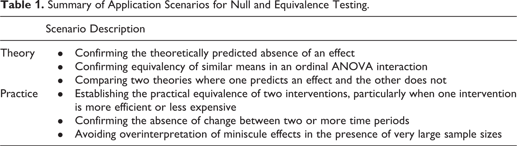
One further application of this thinking lies in avoiding a pitfall of a relatively new issue in organizational research: excess sample size. In some research, the availability of “big data” about employees and organizations can lead to situations where sample sizes are large enough that virtually any effect, no matter how miniscule, achieves statistical significance. From theoretical and practical viewpoints, this raises important concerns—miniscule but significant effects may direct attention and resources to phenomena that do not merit such consideration. In these instances, declaring a threshold for a trivial effect in advance of analyzing data might help to ensure that analytical results are benchmarked against meaningful thresholds. Table 1 summarizes the scenarios described above where null/equivalence testing may be useful.

Table 1.

Summary of Application Scenarios for Null and Equivalence Testing.

	Scenario Description
Theory	• Confirming the theoretically predicted absence of an effect • Confirming equivalency of similar means in an ordinal ANOVA interaction • Comparing two theories where one predicts an effect and the other does not
Practice	• Establishing the practical equivalence of two interventions, particularly when one intervention is more efficient or less expensive • Confirming the absence of change between two or more time periods • Avoiding overinterpretation of miniscule effects in the presence of very large sample sizes

Conducting Equivalence and Null Tests

Applied statisticians have developed several strategies for analyzing data to detect equivalence or to establish credible evidence of no nontrivial effect. The four strategies reviewed below cover a wide range of analytical situations, but for clarity examples using the t test are used throughout the material below. Readers may consult the provided references for more detailed support on applying these techniques in other analytical situations. The Supplemental Appendix contains R code examples demonstrating several other common statistical tests. All of the techniques described below presuppose a research design and data collection amenable to conducting an equivalence test (see Cashen & Geiger, 2004; Cortina & Folger, 1998; Frick, 1995; and Wellek, 2010). For example, the research design must guard against threats to validity, must have sufficient statistical power, and must use appropriate measurement techniques. Additional recommendations on research design appear in the discussion.

Prerequisite: Choosing the Threshold for a Trivial Effect

An important prerequisite to using some of these techniques lies in selecting the threshold for a trivial effect. The terminology section at the beginning of the article introduced the idea of “no nontrivial effect” as described by Cortina and Folger (1998), Cashen and Geiger (2004), and others. Like choosing a power level, setting a threshold for the difference between a trivial effect and a nontrivial effect depends upon the nature of the research. Ideally, a minimum threshold, expressed as an effect size, indicates the strength of effect below which a null hypothesis or hypothesis of equivalence would be considered supportable. Likewise, if a hypothesis predicted a certain minimum effect size, but we obtained a trustworthy finding lower than this minimum threshold, this could be interpreted as evidence for refutation of the hypothesis.

Procedures for choosing minimum thresholds are not routinely taught in organizational science statistics courses. While discussion of this topic began some time ago (e.g., Serlin & Lapsley, 1985; Walster & Cleary, 1970), much early guidance discussed only the statistical techniques for equivalence, leaving the choice of thresholds to readers. Some sources suggest rules of thumb in the form of fixed thresholds for specific statistical tests. For example, Wellek (2010, p. 16) offered d = ±0.36 for the two independent samples t test based on conventions used in bioequivalence testing. As a reminder, Cohen’s d is a common measure of effect size showing the extent of difference between two means and expressed in standard score units (Piasta & Justice, 2010). Frick (1995) suggested that Cohen’s (1992) effect size tables could be used to set equivalence boundaries: Frick’s idea was to set the equivalence boundary just below the threshold of what Cohen deemed as a small effect (for two independent samples, the threshold would be d = ±0.20).

Other researchers recommend choosing equivalence thresholds based on the research context. Lakens et al. (2018) summarized ideas for determining the “smallest effect size of interest” by considering two broad categories: objective and subjective. Objective justifications for a minimum effect size can occasionally be found in areas such as neuroscience because of the quantifiable nature of some research phenomena (e.g., Rinderknecht et al., 2018). In such areas, measurements of a phenomenon may have well-documented ranges that could be used to derive a minimum effect size of interest. In the organizational sciences, however, such ranges are rarely so well defined or documented. As a result, organizational scientists must generally use subjective strategies for setting minimum effect size thresholds.

Prior research can inform subjective thresholds for equivalence when results have revealed effect sizes pertinent to the phenomenon under consideration, but no simple, formulaic method exists for translating previously observed effect sizes into equivalence boundaries. Two of the strategies summarized by Lakens et al. (2018) have notable drawbacks.

First, in areas where meta-analysis has documented a mean effect size for a statistical relationship, one might choose an equivalence boundary based on the lower end of a confidence interval around the meta-analytic effect size estimate. For example, a meta-analysis might show a mean Cohen’s d = 0.35, with a confidence interval ranging from 0.33 to 0.37. The researcher testing an equivalence hypothesis might then set equivalence boundaries to d = ±0.33. This could work in circumstances where meta-analytic findings are homogeneous. An anonymous reviewer pointed out, however, that studies in areas with theoretically meaningful boundary conditions may exhibit more heterogeneous results. In this case, effect sizes for competently conducted studies could show credible and substantively important effects that fall underneath the lower bound of a meta-analytic confidence interval.

Second, Lakens et al. (2018) also raised the possibility that resource constraints on the design of a study might imply an implied minimum effect size that researchers are seeking, based on conventional thresholds for alpha and power. For example, if sample size for a study is limited by resource or logistical constraints, this implies a minimum effect size that could be detected with statistical power of 0.80 and an alpha = .05 (Cohen, 1969, p. 15; Lenth, 2007; Rosnow & Rosenthal, 2008). As the simulation below will show, however, achieving sufficient statistical power to find evidence for a null/equivalence hypothesis often demands much larger sample sizes than detecting the presence of a substantive statistical effect (i.e., support for an alternative hypothesis). Therefore, choosing equivalence boundaries based on resource constraints may easily lead to a study with insufficient power to detect equivalence.

In the absence of a formulaic method for setting equivalence boundaries, researchers should rely on a careful reading of the literature to set reasonable initial boundaries and then consider a sensitivity analysis to explore the robustness of equivalence results. Rules of thumb for equivalence (e.g., Frick, 1995; Wellek, 2010) lack the contextual information on effect sizes provided by the literature and should not serve as the basis for choosing equivalence boundaries. Equivalence boundaries should generally not be set higher than the smallest significant effect observed in a competently conducted previous study. When consulting meta-analytic results, tests of heterogeneity can guide the decision of whether and how to use the lower bound of the confidence interval: Where effect sizes are heterogeneous, the lower bound of the confidence interval may be too large to serve as an appropriate choice for an equivalence boundary.

A sensitivity analysis approach is sensible when there is insufficient evidence from prior literature to settle on one particular equivalence threshold. Rather than choosing just one set of equivalence boundaries, such as d = ±0.3, a researcher can conduct equivalence analyses by repeating the tests at several levels. For example, if a study was designed with sufficient power to detect a null effect with equivalence boundaries of d = ±0.3 and power of .80, one might begin the analysis with a more stringent test at d = ±0.2, proceed to test at d = ±0.3, and conclude with d = ±0.4. The smallest effect size for which equivalence was confirmed would serve as guidance for future replications. Naturally, conducting multiple tests will increase the chances of a false positive and it would be important to acknowledge this possibility in the research report.

Demonstrating the Four Techniques With Real Data

Having settled on a minimum effect size, we can demonstrate null hypothesis and equivalence testing with data. The examples below use an excerpt of data from a previously published article with permission of the data owner (Stanton et al., 2001). The demonstration data contain n = 540 surveyed workers who reported gender and work-related stress appraisal using a validated, multi-item measure. A literature review in the area of work-related stress revealed a meta-analysis that considered gender differences in several stress measures (Davis et al., 1999). This meta-analysis provided guidance for choosing a minimal effect size of interest. Meta-analytic results considering gender differences in stress appraisal showed a confidence interval for effect size that when converted to Cohen’s d amounted to d = 0.303 on the smaller end of the interval. These results were homogeneous for representative samples of adults. Therefore, for the analyses presented below, d = ±0.3 was chosen as the threshold for the smallest effect that would be considered nontrivial.

The demonstration data contained a roughly balanced number of observations for men (n = 298) and women (n = 242) and had two missing values on the stress appraisal measure. The two missing data values were mitigated with mean substitution. A standard power analysis showed that when using an alpha level of .05, a t test with n = 242 per cell had power of 0.91 to detect an effect of d = 0.3 or larger. Note that the material below contains additional considerations of statistical power. Stress appraisal was calibrated on a scale ranging from 8 to 21. The standard deviations for men (SD = 3.5) and women (SD = 3.2) were slightly different, so tests assuming unequal variance are used throughout. The mean for men was 17.82, while the mean for women was 17.96. A Welch’s two-sample t test of gender differences on this measure revealed t(530.7) = –0.497, ns, with an observed p value of .62. Expressed as a mean difference in the metric of the original scale, the confidence interval centered on –0.14 and ranged from –0.70 up to 0.42. Expressed as Cohen’s d, the parallel values are –0.043 for the center and –0.21 and 0.13 for the lower and upper bounds. Taken together, this evidence indicates a failure to reject the null hypothesis.

The analyses demonstrated below seek to affirm whether the comparison of stress appraisal between men and women amounts to practical equivalence. To make the presentation as accessible as possible, the analyses below focus on comparisons of means by gender using the independent samples t test; the extension of these techniques to evaluating other statistical tests is generally straightforward. The Supplemental Appendix includes R code to conduct equivalence tests of correlation coefficients, multiple regression coefficients, and ANOVA effects.

Two One-Sided Tests

The two one-sided tests (TOST) method, first described by Schuirmann (1987) and based on earlier work by Westlake (1976), conducts a pair of one-tailed NHSTs. Contemporary guidance on the use of TOST appears in Limentani et al. (2005), Walker and Nowacki (2011), and Lakens et al. (2018). The TOST procedure conducts two “bookend” NHSTs to ascertain whether the observed point estimate falls inside the selected equivalence boundaries. TOST takes advantage of the fact that it is straightforward to conduct a one-tailed NHST in reference to any arbitrary point on the number line (often expressed in the standard formula for the t test as the value for mu).

The lower and upper bounds for the trivial effect are Cohen’s d values of –0.30 and +0.30. In the first of the two one-sided tests, we conduct a one-tailed NHST on the alternative hypothesis that the mean difference in the population is lower than +0.30, the upper end of the equivalence band. In the second of the two one-sided tests, we conduct a one-tailed NHST on the alternative hypothesis that the mean difference is higher than –0.30, the lower end of the equivalence band. If we confirm both alternative hypotheses we have, in effect, bracketed the effect size somewhere between d = –0.30 and d = 0.30 using two standard inferential tests.

Conveniently, Lakens (2017) developed an R package called “TOSTER” that bundles the two one-sided tests into a single procedure with helpful text and graphical output. In addition to supporting several flavors of the t test, the package also supports TOST procedures for correlation coefficients, meta-analytic effect sizes, and comparisons of two proportions. For the stress appraisal measure, running the TOSTER procedure for two independent samples yields a tabular display with the contents shown in Table 2.

Table 2.

Output for Two One-Sided Tests Procedure for Two Independent Samples.

	Observed t	Degrees of Freedom	p Value
Standard t test	0.497	531	.619
TOST upper	–2.99	531	.001
TOST lower	3.98	531	<.001

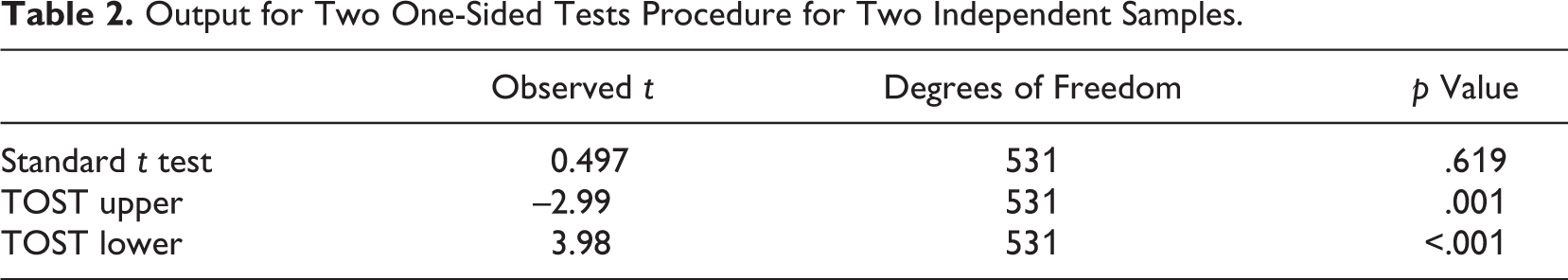
The three rows of Table 2 correspond to the standard NHST t test, the one-tailed test of the upper bound of the trivial range, and the one-tailed test of the lower bound of the trivial range. The degrees of freedom in all three cases refers to the adjusted value used in the Welch’s t test (assuming unequal variances). In the first row, the p value for the standard NHST t test confirms that the difference in means between men and women was not statistically significant. The two subsequent rows in Table 2 indicate that the observed mean difference is both significantly lower than d = 0.30 and significantly higher than d = –0.30. Lakens et al. (2018) noted that there does not need to be a significance adjustment for multiple tests because the TOST upper and TOST lower tests must both be significant for equivalence to be supported. Other elements of the output (not shown in Table 2) report the equivalence boundaries, confirming the –0.30/+0.30 range we specified for Cohen’s d. Keeping in mind that Cohen’s d is a standardized measurement, we may also wish to know the equivalence bounds expressed in the metric of the original variable. The procedure calculated these values as –0.996 to 0.996. These results support a hypothesis of equivalence in self-reported stress appraisal between men and women.

Inference by Intervals

Inference by intervals was a concept suggested by Westlake (1976), Dunnett and Gent (1977), Freedman and Spiegelhalter (1983), and others as a consideration of the equivalence of treatments in biomedical research. Freedman and Spiegelhalter addressed a question that is common in clinical research: Using an interim analysis when a trial is under way, a statistical “stopping rule” determines when clinical researchers can conclude that a new treatment is definitively better (or worse) than an existing one. The method that Freedman and Spiegelhalter proposed was to establish an equivalency band—a range of equivalence around a difference of zero—within which a trial would continue to treat patients and collect data. Once the entirety of the observed confidence interval of the difference between the old and new treatments fell outside of this band of equivalence, the new treatment would be considered effectively different from the old one. Dienes (2014) and Tryon (2001; Tryon & Lewis, 2008) refined the techniques and provided more details on decision rules. Figure 1 displays a hypothetical set of confidence intervals—all calibrated in Cohen’s d—that illustrate a range of relevant scenarios. Scenario numbers appear on the x-axis.

Figure 1.

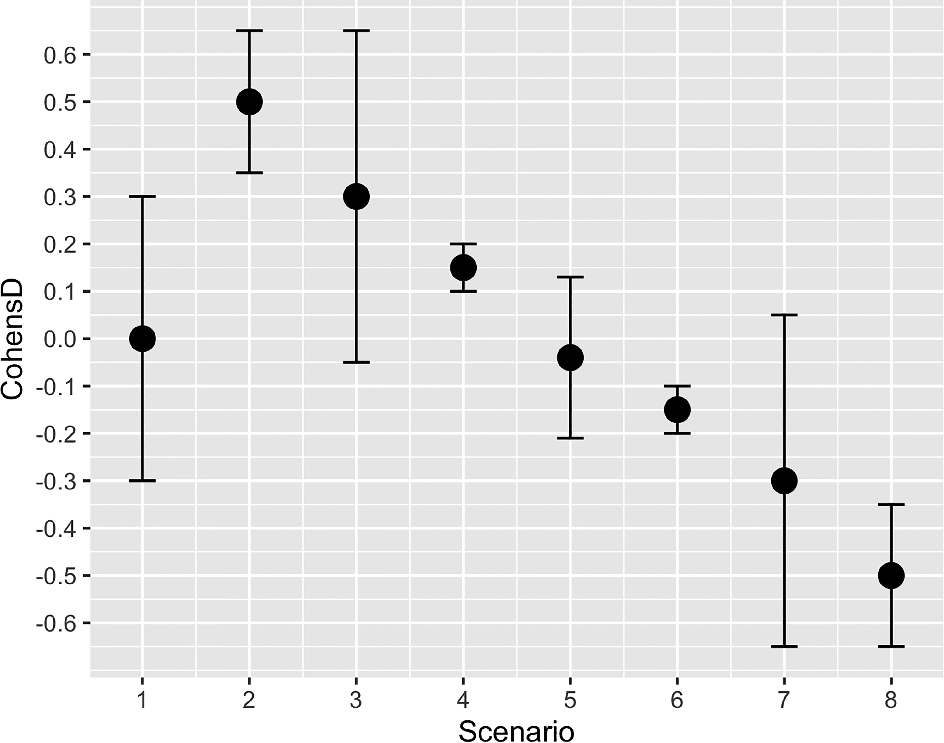
Different Scenarios for Inference by Intervals.

In Figure 1, on the far left, Scenario 1 shows the band of equivalence (i.e., no nontrivial effect) selected by the researcher; it therefore does not depict a calculated confidence interval as such. Consistent with this demonstration, the equivalence band runs from d = –0.30 to d = 0.30. The differing widths of confidence intervals for Scenarios 2 through 8 denote the idea that several different sample sizes might be under consideration or that different tested variables might have a variety of variances (or both). Scenario 2 shows a strong positive effect size that would be statistically significant using the NHST. Obtaining a finding like Scenario 2 would cause a clinical trial to stop because the new treatment would be considered definitively better than the standard treatment (Freedman & Spiegelhalter, 1983). Scenario 3 is “statistical limbo,” in that the NHST would fail to reject the null and yet the confidence band also includes an interval with nontrivial effects. Scenario 4 shows a paradoxical finding that hearkens to the excess sample size scenario described earlier—the NHST would be statistically significant, but one would nonetheless consider this a trivial effect and inference by intervals would deem it as such. Finally, Scenario 5 demonstrates confirmation of a hypothesis of equivalence: The confidence band is contained entirely inside the +0.3/–0.3 range of a trivial effect and the NHST would be nonsignificant due to the overlap with zero. Scenarios 6, 7, and 8 show the equivalent findings to Scenarios 4, 3, and 2, respectively, for negative values of Cohen’s d.

In our demonstration example of gender differences in stress appraisal, the observed confidence interval for the difference in stress appraisal was centered on a Cohen’s d value of –0.043, considered a negligible effect by typical standards. The cohen.d() function from R’s “effsize” package converted the raw data into a Cohen’s d confidence interval. The confidence interval expressed as Cohen’s d ranged from –0.21 to 0.13. This observed confidence interval fits inside the –0.3/+0.3 equivalence boundaries. In Figure 1, the confidence band shown for Scenario 5 represents the precise results reported here for gender differences in stress appraisal. We can thus conclude, based on inference by intervals, that men and women indicated practically equivalent levels of stress appraisal on the measure used here. Note that the researcher may select any confidence level as the basis for constructing the confidence intervals, such as 90%, 95%, or 99%, based on their preference for the stringency of the test. As the simulation will later show, to maintain compatibility with TOSTER results one must choose a 90% confidence interval.

Bayes Factors

Bayes factors focus on comparing the evidence for two competing hypotheses (Aitkin, 1991; Berger & Pericchi, 1996; Dienes, 2014; Rouder et al., 2009; Stanton, 2017). Although these two hypotheses can compare any pair of statistical scenarios, the typical application is comparing a null hypothesis to an alternative hypothesis. The result, a so-called Bayes factor, is expressed as an odds ratio. Odds ratios near 1:1 provide ambiguous evidence that favors neither of the hypotheses being compared. Strong odds, such 150:1 in favor of the alternative hypothesis, are typically sought by analysts when addressing a substantive research question. To consider an equivalence hypothesis, this thinking is inverted to seek odds ratios in favor of a null finding. The null in this case is expressed as an equivalence interval.

Morey et al. (2015) developed an R package called “BayesFactor” that includes a feature for equivalence testing (also see Rouder et al., 2012). Specifically, in requesting a Bayes factor for a procedure such as a t test, one may specify a null interval to be evaluated in addition to the alternative hypothesis. The resulting output reports two Bayes factors, one for the region within the null interval and one for the region outside of the null interval. These two Bayes factors must be compared with each other to test the viability of the equivalence hypothesis. This comparison is straightforward, as both values are expressed as odds ratios against a common denominator. Divide the Bayes factor for the null interval by the Bayes factor for the area outside the null interval to obtain the odds in favor of the null interval (Morey & Rouder, 2011).

Using the stress appraisal measure to compare gender differences, results showed an odds ratio of 0.42 for the null interval and an odds ratio of 0.00018 for the area outside of the null interval. Dividing the former by the latter provides odds of 2,295 in favor of the null interval, a strong result. In the next section, the simulation will put these odds in perspective and provide a minimum threshold for odds that represent a credible finding of equivalence. The simulation will also compare results emerging from the four techniques.

Bayesian Estimation With HDI and ROPE

The use of Bayesian methods for estimating population values has become more accessible over recent years (Kruschke et al., 2012; Rouder et al., 2009; Stanton, 2017). New methods of estimation and corresponding software packages have made it possible to substitute Bayesian estimation in place of almost every standard NHST test (e.g., t test, F-test, chi-square test, etc.). Bayesian parameter estimation methods produce a distribution of “posterior” estimates of population values of interest from which the researcher draws inferential conclusions. In this context, the term “posterior” refers to one of the elements of Bayes’ theorem. For our purposes, the posterior distribution can provide insights that are conceptually akin to a confidence interval, but with richer detail about the likely location of the population value under consideration.

When testing the stress appraisal measure, a Bayesian t test developed by Kruschke (2013; the “BEST” package for R) produced a distribution of about 100,000 posterior estimates of the mean difference by gender. This posterior distribution was normally distributed and centered on a mean difference of –0.13. In the context of Bayesian parameter estimation, analysts use the term “highest density interval” (HDI) to refer to the central region of this distribution. Under the logic of Bayesian estimation, the HDI is said to include the range of most likely population values, given prior assumptions about the population and the available data sample. Kruschke (2011) coined the term “region of practical equivalence” (ROPE) to refer to an HDI that one could use to assess a hypothesis of equivalence. In the case of our stress appraisal example, we established boundaries for ROPE calibrated in Cohen’s d as –0.30/+0.30 with equivalent raw data values of –0.996 and 0.996. To establish whether the bulk of the posterior distribution lies within this ROPE, we calculated the proportion of 100,002 posterior estimates that fell within this –0.996 and 0.996 region. The calculation (see Supplemental Appendix) revealed that about 99.8% of the posterior estimates fell within this region. This result provides credible evidence of no nontrivial difference between the men and women on stress appraisal.

Comparing the Four Methods via Simulation

The four equivalence test methods demonstrated above share the high-level goal of ascertaining whether a population value of interest, such as a mean difference, may lie inside a set of equivalence boundaries. In the example described above, using real data to compare two independent means, evidence from all four techniques led to the same conclusion, that a measure of workplace stress appraisal was practically equivalent between men and women. Yet it is also important to understand how the four techniques may differ from one another in the results they produce across a range of research situations. As such, a Monte Carlo simulation can provide insight into which technique to choose in different circumstances by testing the techniques with a large variety of random samples. Of related interest, a simulation can uncover the decision criteria needed to ensure consistency of results, regardless of the selected technique.

The simulation described below occurred in two phases—one phase focusing on sampling from one population and a second phase focusing on sampling from two populations with an effect size (difference in means) equal to the equivalence boundaries used in the tests. In the first phase, the goal was to understand true positives: the long run capability of the equivalence tests to detect, correctly, a null effect or finding of equivalence. In the second phase, the goal was to understand true negatives, that is, the capability of each test to avoid indicating equivalence when a statistical effect was, in fact, present. In both phases, recommendations from Carsey and Harden (2014) guided the choice of operational parameters for the simulations—for example, 10,000 tests were conducted for each sample size within each phase to ensure the stability of the results. Each phase considered five different sample sizes based on statistical power considerations. At the low end, n = 50 observations for each of two groups provided very low statistical power, while n = 800 per group provided very high power. The first row of Table 3 (t power, d = 0.3) shows the power of the independent samples t test to detect an effect size of d = 0.3 given the group size indicated in the column. All of the findings displayed in Table 3 represent samples drawn from normal populations with standard deviations equal to one. At the conclusion of this section, an additional discussion reviews results from other distributions.

Table 3.

Results of Monte Carlo Simulation.

	Sample Size per Group (Overall df Shown in Parentheses)
Simulation Results	n = 50 (df = 98)	n = 100 (df = 198)	n = 200 (df = 298)	n = 400 (df = 798)	n = 800 (df = 1,598)
t power, d = 0.3	0.32	0.56	0.85	0.99	0.99
Null power, d = 0.3	0.00	0.37	0.82	0.99	0.99
TOST correct % (true effect d = 0)	0%	36.9%	81.6%	99.2%	100%
Inf. int. correct % (true effect d = 0)	0%	36.9%	81.6%	99.2%	100%
Bayes factor 50 (true effect d = 0)	0%	43.9%	84.7%	99.2%	100%
Bayes 90% HDI (true effect d = 0)	0%	44.2%	84.1%	99.2%	100%
TOST correct % (true effect d = 0.3)	100%	94.9%	95.2%	94.4%	95.5%
Inf. int. correct % (true effect d = 0.3)	100%	94.9%	95.2%	94.4%	95.5%
Bayes factor 50 (true effect d = 0.3)	100%	93.2%	93.1%	93.1%	94.1%
Bayes 90% HDI (true effect d = 0.3)	100%	93.8%	94.1%	93.7%	95.1%

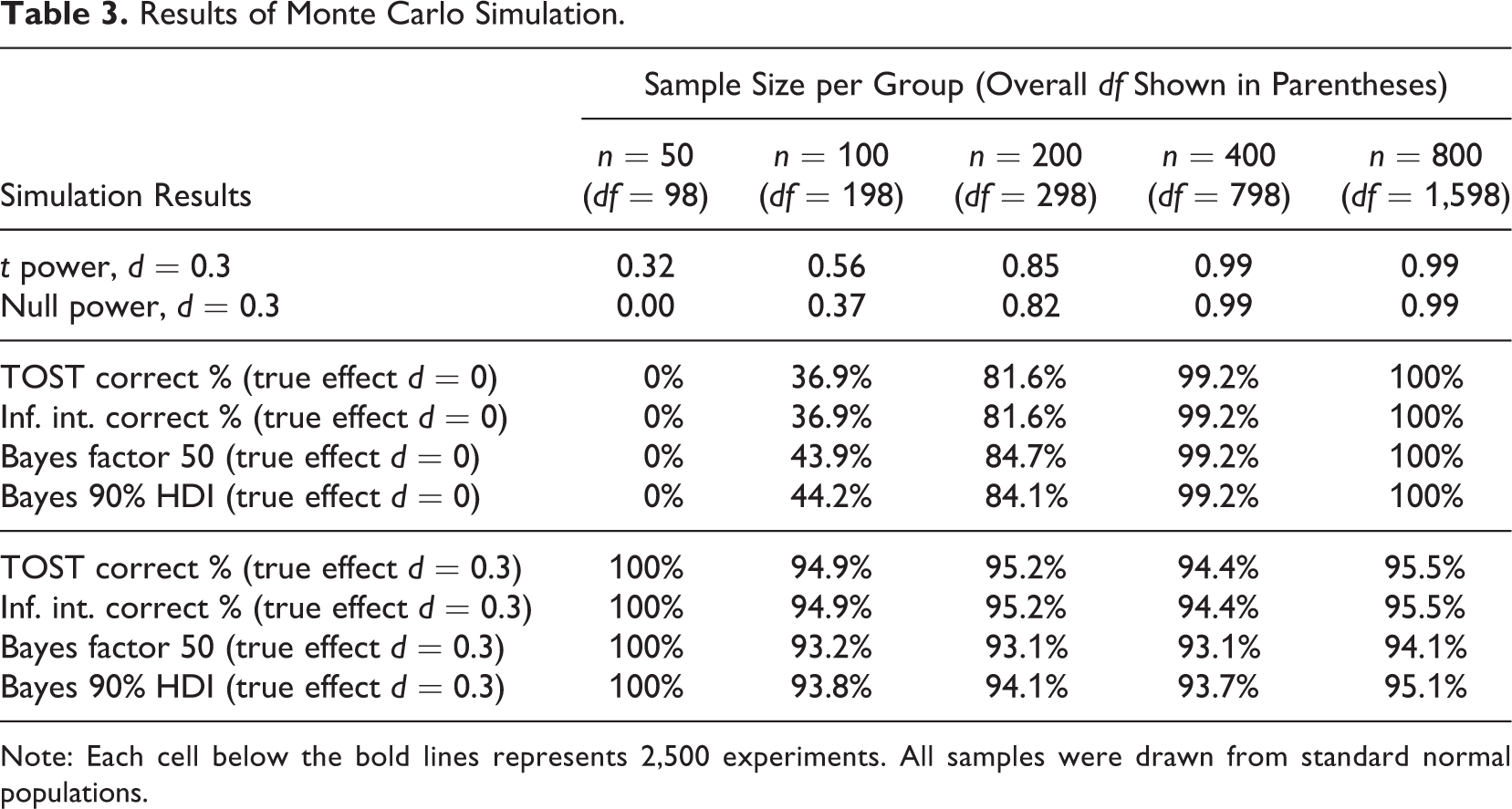
Note: Each cell below the bold lines represents 2,500 experiments. All samples were drawn from standard normal populations.

The TOSTER package provides a procedure that previews the power of an equivalence test. This power calculation differs from that of the regular t test as shown in the second row of Table 3 (null power, d = 0.3). With small samples, the power for equivalence testing is lower than the power of the standard NHST (Chow et al., 2017, p. 62). Table 3 shows that with group sizes smaller than n = 200, the power of an equivalence test to detect practical equivalence with bounds of d = ±0.3 was unacceptably low.

Underneath the first bold line, Table 3 contains four lines of data, one for each of the equivalence tests. Each cell represents an outcome from 2,500 experiments, where two samples were drawn from the same population. The values shown in each cell represent the percentage of correct decisions by the respective procedure at various sample sizes. A correct decision in these cases was the indication of equivalence between the two samples, using equivalence bounds of d = ±0.3. The TOST procedure and inference by intervals (using a 90% confidence interval) provided identical results in all cases. At sample sizes near n = 100, the two Bayesian methods outperformed the two frequentist methods. This advantage disappeared at larger group sizes.

An important finding of the simulation was that the closest match between the Bayesian estimation method and the other techniques occurred when the HDI for the region of practical equivalence was set at a threshold of 90% of the posterior estimates. In other words, to pass the test and support a hypothesis of equivalence, 90% of the posterior distribution needed to fit within the equivalence bounds of d = ±0.3. Previously, Kruschke (2011) had suggested that 95% was the most appropriate value to use. The simulation showed that 90% was the more appropriate choice, if accuracy of detecting practical equivalence was the primary goal. Choosing a more stringent criterion such as the 95% HDI would improve performance in rejecting false positives but would decrease the true positive rate.

Another important finding from this phase of the simulation was that the closest match between the Bayes factor method and Bayesian estimation was achieved when the decision threshold for the Bayes factor was set to odds of 50:1 in favor of the null interval. Using this odds ratio, the two Bayesian methods agreed in 98% of the tested samples. To put this odds ratio in perspective, Kass and Raftery (1995) suggested that for the evaluation of a typical research hypothesis, any odds ratio weaker than 3:1 is too weak to mention, odds ratios between 3:1 and 20:1 constitute positive evidence for a hypothesis, ratios from 20:1 up to 150:1 are strong evidence, and any odds ratio in excess of 150:1 is considered very strong evidence for the hypothesis. Thus, the simulation demonstrated that when using the Bayes factor as a basis for making decisions about equivalence, one must use a more stringent criterion than one might use for the evaluation of a typical research hypothesis.

One final note for this phase of the simulation is that the accuracy values shown in each cell of the middle of Table 3 also represent the observed statistical power of each technique for the given sample size, insofar as subtracting the value in a given cell from 100% gives the false negative rate for that test (often referred to as beta). Compare the power values documented in the second row of Table 3 to these four rows to understand how the respective technique performed relative to the theoretical power to detect equivalence.

In the second phase of the simulation, displayed under the lower bold line of Table 3, each cell also represents 2,500 tests, where the two samples were drawn from different populations. The means of the two populations were set to be d = 0.30 apart, such that a correct decision would be that equivalence does not exist (using bounds of d = ±0.30). Setting the mean difference between the two populations to precisely the same value as the equivalence bounds provides the conditions for assessing the worst-case scenario with respective to false positives. Note that at the smallest sample size (n = 50 per group), all of the techniques failed to find evidence of equivalence in 100% of the tests. Yet this must be considered a trivial result because of the low statistical power at this sample size.

For all of the other sample sizes, the typical correct decision rate hovers near 95%. These values represent the specificity of each test at the specified sample size. As such, the statistical threshold that we typically refer to as alpha can be computed as 100% minus the accuracy value shown in this section of the table. This means that in about 5% of the simulation experiments for group sizes of n = 100 and larger, samples were drawn that seemed to indicate a finding of equivalence even though the population means were in fact d = 0.3 apart (a false positive).

One finding from this second phase of the simulation is that the two Bayesian techniques—using the same decision criteria as described above—underperform the frequentist techniques by about one to two percentage points at smaller sample sizes. The sensitivity of these Bayesian tests could be improved by using more stringent decision criteria (e.g., 95% HDI of posterior estimates for Bayesian estimation or an odds ratio of 60:1 for Bayes factor), at the cost of diminishing the true positive rates documented in Phase 1 of the simulation.

Not shown in Table 3 are the results of running the simulation on nonnormal populations. Three additional sets of distributional scenarios were created for each sample size, with population effect sizes of d = 0 and d = 0.3 assessed separately for each scenario. The goal of running these additional scenarios was to evaluate whether the accuracy of the equivalence testing techniques would be adversely affected when sample data were nonnormal. In the first scenario, two populations with skewness of +1 were compared, while in the second scenario, one population had a skewness of +1 whereas the other population had skewness of –1. In the third scenario, two populations with uniform distributions were compared.

None of the four equivalence testing techniques was adversely affected by these nonnormal distributions, with respect to their true positive performance. Interestingly, the specificity of the four techniques (their ability to avoid false positives) actually improved when testing skewed populations, particularly when the skewness went in opposite directions for the two populations. The presence of greater proportion of observations in the tails of these distributions made it easier for the techniques to avoid a false conclusion that equivalence existed between the different populations.

Finally, running the simulation across all of these scenarios provided the opportunity to document the performance of the four techniques across a variety of samples and distributions. As suggested by the results in Table 3, the Bayesian techniques outperformed the frequentist techniques at detecting true positives. Averaged across all sample sizes and all distributions, the Bayesian techniques correctly detected 2% more findings of equivalence. In terms of correctly rejecting equivalence when the two populations were different, the four techniques were all within half a percentage point of each other, when averaged across all sample sizes and distributions. In absolute terms, the Bayes factor method, using a threshold odds ratio of 50, was the single best technique, although its performance was only trivially better than Bayesian estimation, when using a 90% HDI as the region of practical equivalence.

Discussion

This article reviewed four techniques for obtaining credible evidence to confirm a null hypothesis or show practical equivalence, for example, between two mean values. The TOST procedure and inference by intervals share frequentist roots and a focus on positioning a sample statistic within a prespecified band of equivalence. Simulation results demonstrated that these two techniques produce identical conclusions under all circumstances.

The Bayes factor method and Bayesian estimation of a region of practical equivalence both have their origins in Bayesian thinking. Simulation results showed that these tests produce similar results to each other. With smaller samples, the Bayesian techniques performed better than the frequentist techniques at correctly detecting equivalence when it was present. In those same smaller samples, the frequentist techniques performed slightly better at avoiding false positives. Given these trade-offs, choosing which technique to use and report may depend partly upon the audience for the results. Kruschke et al. (2012) reported that most journals in the organizational sciences have 2% or fewer articles that include Bayesian methods. The TOST procedure, paired with inference by intervals, may have greatest appeal for readers and within journals that generally use the NHST.

Table 4 summarizes the guidance for conducting these techniques that was derived from the Monte Carlo simulation and the prior research literature. The table shows nine steps beginning with planning the study and concluding with analysis and reporting of results.

Table 4.

Null/Equivalence Testing Steps and Decisions.

Step	Frequentist	Bayesian
1. Design for null testing	Confirm validity considerations and measurement strategy. Operationalize key variables that will be used in equivalence tests in more than one way. In addition to the variables for equivalence testing, include an additional independent variable that is predicted to have a credible, nontrivial effect.
2. Choose equivalence boundaries	Use prior empirical results where available to choose equivalence boundaries for the test. Consider sensitivity analysis that examines several equivalence boundary levels.
3. Conduct power analysis for equivalence testing	TOST power estimation procedures in the TOSTER package give conservative values for the power of equivalence tests. With larger samples, the power of the Bayesian procedures will be the same as frequentist procedures. With smaller samples the Bayesian procedures provide slightly higher power.
4. Set target sample size	Use the power analysis to guide data collection targets. Sample sizes for null/equivalence testing generally exceed those needed for regular hypothesis testing. The narrower the equivalence interval, the larger the sample size must be to achieve acceptable power.
5. Choose Bayesian or frequentist	The TOST and inference by intervals techniques are easier to explain to those familiar with the NHST and may be the preferred choice at some journals.	For readers familiar with Bayesian techniques, the Bayes factor procedure provides the best overall performance across various sample sizes and distributions.
6. Conduct the test and assess the equivalence interval	TOST provides a go/no-go decision based on two one-sided tests that bracket the equivalence interval. Use inference by intervals to construct a 90% confidence interval around the sample estimate. That result graphically illustrates the same conclusion as the TOST procedure.	Odds ratios from the Bayes factor procedure greater than or equal to 50:1 provide an ideal balance between power and sensitivity. The 90% HDI from Bayesian estimation offers an interval representation that complements the Bayes factor.
7. Describe equivalence hypothesis	Discuss the theoretical and/or practical basis for conducting the test of equivalence. Indicate what measure(s) were used for testing and the rationale for choosing either frequentist or Bayesian techniques.
8. Report boundaries and power analysis	Describe the considerations used to decide on the equivalence boundaries and state those boundaries, generally using a standardized measure of effect size such as Cohen’s d. Report the prestudy power analysis and, if sample size changed from planned goal, an updated power value.
9. Report decision and interval	Report the results of the TOST procedure and indicate whether the equivalence hypothesis was supported. Report upper and lower boundaries of the 90% confidence interval for inference by intervals.	Report the observed Bayes factor and comment on the strength of the result relative to the threshold odds of 50:1. Calculate percentage of posteriors within the 90% HDI from Bayesian estimation.

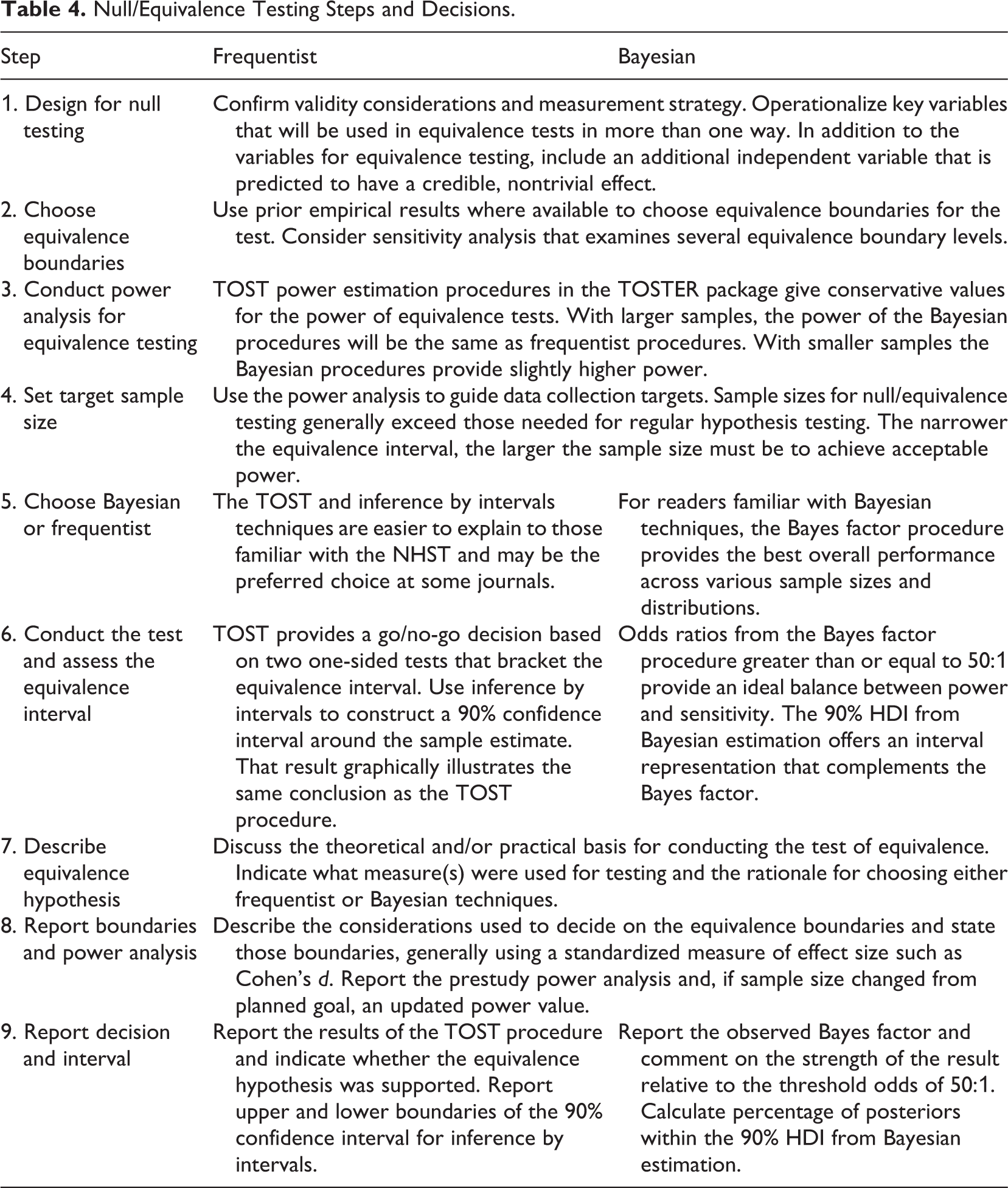
Prior to developing sample size goals and an analysis plan for equivalence testing, researchers should consult Cortina and Folger (1998), Cashen and Geiger (2004), or Wellek (2010) for guidance on measurement and study design. Cashen and Geiger (2004, p. 162) synthesized prior literature into two design recommendations that are important to reiterate here. First, in an ideal research design, the statistical tests confirming equivalence should be conducted on more than one operationalization of the relevant variables. An equivalence finding that replicates on more than one measure of the construct or constructs of interest carries more weight. Second, a research design should ideally contain an additional independent variable that can be shown to have a nontrivial and statistically significant effect on the dependent variable of interest. This additional variable serves as an existence proof that it is possible to confirm a typical alternative hypothesis using the dependent variable in question, thereby making a clear contrast with a successful equivalence test.

Choosing equivalence boundaries can be guided by previous research results, assuming a suitable set of prior findings exists. Meta-analytic confidence intervals can provide guidance when reported effect sizes are shown to be homogeneous. When it is not possible to make a definitive choice, use sensitivity analysis to test multiple thresholds for equivalence.

Statistical power to detect equivalence will depend in part upon the selected width for the equivalence band: Finding equivalence within a narrower band will require a larger sample. Table 5 shows the minimum sample size per group needed to achieve power of 0.80 in a comparison of two group means. Separate columns show values for TOST / inference by intervals and Bayes factor techniques. For tests of equivalence bands of d = ±0.3 or less, TOST and inference by intervals require higher sample sizes. Results from the middle section of Table 3 showed that the power calculations from the TOSTER package matched the simulations of the frequentist techniques and were slightly more conservative than the power exhibited by the Bayesian techniques. Therefore, the eight functions offered by TOSTER for calculating the power of equivalence tests can be used without underestimating power. Consult Rusticus and Lovato (2014) for additional power simulations for equivalence testing and Kruschke and Liddell (2018) for more insights into statistical power for Bayesian techniques.

Table 5.

Minimum Group Sizes Needed to Detect Null/Equivalence With Power = .80.

Equivalence Boundaries: Cohen’s d	TOST Group Size	Bayes Factor Group Size
d = ±0.1	1,710	995
d = ±0.2	430	360
d = ±0.3	190	175
d = ±0.4	110	105
d = ±0.5	70	70
d = ±0.6	50	50
d = ±0.7	35	35
d = ±0.8	30	30
d = ±0.9	20	20
d = ±1.0	20	20

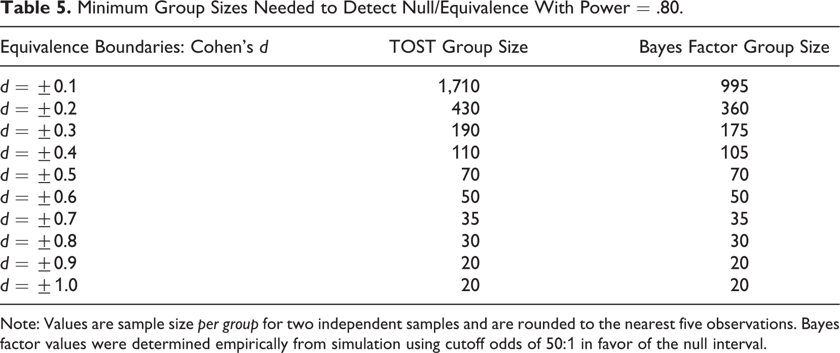
Note: Values are sample size per group for two independent samples and are rounded to the nearest five observations. Bayes factor values were determined empirically from simulation using cutoff odds of 50:1 in favor of the null interval.

After the study planning stage, create an analysis plan for testing equivalence or confirming the null. This article demonstrated techniques for comparing sample means and focused on assessments of the Cohen’s d effect size statistic. The code in the Supplemental Appendix also demonstrates techniques for confirming the null hypothesis or an equivalence interval for a correlation coefficient, a regression weight, and an ANOVA factor. In principle, one can conduct null/equivalence testing on any effect size statistic for which a confidence interval can be calculated. Choosing between the Bayesian or frequentist analysis techniques depends partly on the expectations of the audience for the research results. For those preferring the NHST, pairing the TOST with inference by intervals makes sense because these two techniques provide identical results under all circumstances. TOST provides a go/no-go decision that is simple to explain; inference by intervals backs up the TOST decision with a 90% confidence interval that can provide a graphical depiction of whether and how the observed interval fits within the equivalence boundaries that were set prior to conducting the study. Just as editorial policies for some journals request the use of confidence intervals to complement the results of the NHST, the same logic applies here. TOST and inference by intervals provide consistent and complementary information about an equivalence test, so both should be reported. Another advantage of using TOST together with inference by intervals is that these techniques can be applied without having access to the raw data, as long as the available research report provides information about group size, means (or other appropriate values), and standard deviations of relevant measures.

Table 4 shows a parallel path for the Bayesian techniques in Steps 5, 6, and 9. The Bayes factor technique—which had the best performance among the four techniques—provides a calculated odds ratio showing the odds in favor of the null interval. The simulation showed that a decision threshold for the odds ratio of 50:1 provides a workable balance between the power and sensitivity of the procedure. Using this threshold as the basis for a go/no-go decision on equivalence provides a conceptual parallel to TOST, with slightly better overall performance. To accompany the Bayes factor, the results of Bayesian estimation can produce a 90% HDI, which bears some conceptual similarities to a frequentist confidence interval. Calculating and reporting the 90% HDI complements the results of the Bayes factor analysis by showing whether and how the distribution of posterior estimates fits within the equivalence boundaries that were set prior to conducting the study. For example, examining the boundaries of the HDI might show that the posterior distribution protrudes slightly past the lower bound but is also well underneath the upper bound, a finding that could inform a directional hypothesis about the expected effect.

Reporting Equivalence Testing Results

Steps 7, 8, and 9 of Table 4 indicate that best practices for reporting equivalence results or confirmations of a null hypothesis would always begin with a justification of the equivalence hypothesis. This justification would include references to theory and/or practice as appropriate to the area of research. Next, the report should indicate the selected equivalence boundaries, preferably expressed as a standardized effect size. That discussion will lead naturally to a description of the results of the power analysis for the equivalence test and an indication of the resulting target sample size.

Best practice for reporting the TOST results would include a report of the t-values, degrees of freedom, and p values for the TOST upper and TOST lower tests. Because the procedure may not be familiar to most readers, it would be useful to explain that both tests must be significant to affirm an equivalence hypothesis or no nontrivial effect hypothesis. Because the inference by intervals results always lead to the same conclusion as the TOST, reporting the observed interval simply provides a complementary view of the equivalence results. Just as many journals request that authors report a confidence interval in addition to a significance test, the combination of TOST and inference by intervals provides readers with two useful perspectives on the results of the equivalence test.

Reporting a Bayes factor test of a null/equivalence hypothesis could include a report of both the odds ratio for the null interval and the odds ratio for the area outside of the null interval and finally, for the reader’s convenience, the results of dividing the former by the latter, as illustrated in the real data example. The simulation results led to a recommendation of choosing an odds ratio of 50:1 as the minimum threshold to confirm a hypothesis of equivalence. In virtually all cases, an evaluation of the Bayesian estimation results by constructing a 90% HDI for the posterior distribution will lead to the same conclusion as the Bayes factor procedure. In the occasional case where the two methods disagree, the discrepancy will be minor: either the Bayes factor will be slightly below 50:1, or a small amount of the posterior distribution will protrude past one or both of the 90% HDI boundaries. Either discrepancy would signal a relatively weak finding of equivalence which should be acknowledged as such.

One final consideration related to any Bayesian analysis pertains to the use of priors. The theoretical foundation of Bayesian methods always includes attention to prior probabilities—these encompass what is known about the analytical situation before data are collected and evaluated. Kruschke (2011), Rouder et al. (2009), Morey and Rouder (2011), and others describe the role of priors in Bayesian analysis. Algorithms that implement Bayesian analyses for applied research generally offer a set of default priors that have been shown in simulation to work well across many situations. Kruschke et al. (2012) discussed the use of noncommittal priors and offered procedures for power analysis that illustrated the important impacts of small sample sizes (e.g., n < 50) on Bayesian results. Simulation results in Table 3 showed, however, that it is virtually impossible to detect equivalence at these small sample sizes. As a result, when using the larger sample sizes needed for equivalence testing, default priors will generally suffice.

Limitations and Future Directions

Both the demonstration and the simulation in this article focused on the t test as one of the most essential statistical tests in the researcher’s toolkit. While the Supplemental Appendix contains code that expands the researcher’s options to several other statistical tests, no simulations were conducted on these other tests (e.g., confirming a regression weight to be practically equivalent to zero). It is possible that an expanded simulation containing a greater variety of statistical testing scenarios would provide additional insights into the power, specificity, and error rates of those other tests. Future research could report simulations that demonstrating the use of null and equivalence testing on regression weights, ANOVA effects, tests of proportions, and other kinds of statistical tests. One particularly ripe area for further exploration lies in a host of commonly used confirmatory tests, where we generally prefer to accept a nonsignificant finding (e.g., Bartlett’s chi-square test; see Hayton et al., 2004) as a positive indication of some result.

Another important limitation to keep in mind when conducting null and equivalence testing is that results obtained from a particular sample of data can never be conclusive on their own. Just as we rely on replication over multiple studies together with meta-analysis to cement the strength of a typical research hypothesis, we must expect the same from efforts to establish the absence of an nontrivial effect or a finding of equivalence. Obtaining one set of results supporting a hypothesis of equivalence initiates the discovery process by providing a single piece of evidence, but replication of that finding over multiple studies is needed to strengthen the credibility of any result initially obtained from studying a single sample.

A related issue pertains to the expectations of the research community that reviews those results. While this article demonstrates when one might use null and equivalence testing and how one accomplishes these tests, the question remains of how well a research study designed around an equivalence test might gain traction during the publication process. The norms around conventional hypothesis testing (e.g., the typical choice of alpha = .05) are well established in the organizational sciences, such that they are essentially taken for granted when presented in a research article. The same cannot be said of null and equivalence testing, however, as there are relatively few examples of published research that use the techniques described in this article.

One way to prime the pump would be in statistics education: Integrating null and equivalence testing into graduate statistics curricula would help researchers become more aware of how and when to deploy such tests. A side benefit of learning about null and equivalence testing might be an improved understanding of the importance of statistical power and the need to assess power when designing a study. To support these goals, additional working examples of null and equivalence testing in action are needed, along with exercises for students and guidance to instructors. Relatedly, while packages like TOSTER bundle together several valuable tests for users of R and R-Studio, it would be helpful if other statistical packages offered convenient methods for null and equivalence testing.

Conclusion

Techniques for null/equivalence testing provide opportunities for strengthening organizational research. First, such tests provide an analytical basis for refuting features of existing theories and contrasting predictions of competing theories. Dienes (2014) points out that when researchers test a theoretical proposition and obtain a nonsignificant result, it is difficult to assign responsibility to the theory because of the ambiguities that may underlie such a finding. In contrast, if one follows up a typical hypothesis test with a procedure that provides credible support for a null effect, one accumulates a finding that can add to the weight of evidence against that particular theoretical feature. Solidly supporting a null result does not eliminate other possible sources of problems (such as inadequate measurement or weak experimental manipulations), but it is superior to simply failing to reject the null.

Second, in examining organizational interventions such as training, occupational health interventions, new technology introductions, or changes to organizational structure, having familiarity with null/equivalence testing opens up new possibilities for pinpointing what works, what doesn’t work, and what remains unchanged after critical events have occurred. Most researchers avoid the mistake of interpreting a failure to reject the null hypothesis in a standard NHST test as evidence for no effect or equivalence between two treatments. Yet after encountering a nonsignificant finding, many researchers halt further exploration, leaving their findings in an unnecessarily ambiguous state. In contrast, confirming explicitly that the old, costly training and the new, streamlined training lead to equivalent benefits would in most cases represent a better ending point for a piece of applied research.

Finally, planning ahead for credible confirmations of null effects also requires planning ahead for sufficient statistical power. Serlin and Lapsley (1985) stated that to improve progress in social science research, every research hypothesis should be accompanied by a statement of the boundaries of a “good enough” zone—what Cortina and Folger (1998) and this article have referred to as the threshold between a trivial and a nontrivial effect. Putting this advice into action implies giving forethought to statistical power. If an alternative hypothesis is not supported and there is not enough power to confirm the null, that represents a statistical limbo, where we do not learn anything of value. If there is sufficient power, we have a greater assurance of either supporting the alternative hypothesis or supporting the null. Preparing for null/equivalence testing during study design and conducting these tests during data analysis thus imposes a valuable discipline, because gathering credible evidence for an equivalence hypothesis requires a study design with adequate statistical power.

Without repeating the laments concerning low statistical power in published and unpublished research, ample evidence suggests that the issue is still pervasive (e.g., Aguinis, 1995; Edwards & Berry, 2010; Ferguson & Ketchen, 1999; Halsey et al., 2015). While researchers may choose to explore their alternative hypotheses without specifying an expected effect size, that approach does not work well for null/equivalence testing. Examining a hypothesis of equivalence requires specifying intervals within which such a hypothesis would be supported. Selecting an interval before data collection encourages a consideration of power because sample sizes that are too small cannot establish observed confidence intervals narrow enough to fit within the equivalence band. Incorporating more statistical power from the start of a research design thus improves the quality of the research, increases power for detecting hypothesized effects, and facilitates the null and equivalence testing techniques described in this article.

Supplemental Material

Supplemental Material, Appendix - Evaluating Equivalence and Confirming the Null in the Organizational Sciences

Supplemental Material, Appendix for Evaluating Equivalence and Confirming the Null in the Organizational Sciences by Jeffrey M. Stanton in Organizational Research Methods

Footnotes

Declaration of Conflicting Interests

The author(s) declared no potential conflicts of interest with respect to the research, authorship, and/or publication of this article.

Funding

The author(s) received no financial support for the research, authorship, and/or publication of this article.

ORCID iD

Jeffrey M. Stanton

Supplemental Material

Supplemental material for this article is available online and on the following repository

References

Aguinis

(1995). Statistical power with moderated multiple regression in management research. Journal of Management, 21(6), 1141–1158.

Aitkin

(1991). Posterior bayes factors. Journal of the Royal Statistical Society: Series B (Methodological), 53(1), 111–128.

Barone

M. J.

Norman

A. T.

Miyazaki

A. D.

(2007). Consumer response to retailer use of cause-related marketing: Is more fit better? Journal of Retailing, 83(4), 437–445.

Berger

J. O.

Pericchi

L. R.

(1996). The intrinsic Bayes factor for model selection and prediction. Journal of the American Statistical Association, 91(433), 109–122.

Carsey

T. M.

Harden

J. J.

(2014). Monte Carlo simulation and resampling methods for social science. Sage.

Cashen

L. H.

Geiger

S. W.

(2004). Statistical power and the testing of null hypotheses: A review of contemporary management research and recommendations for future studies. Organizational Research Methods, 7(2), 151–167.

Chow

S. C.

Shao

Wang

Lokhnygina

(2017). Sample size calculations in clinical research. Chapman & Hall/CRC.

Clay-Warner

Reynolds

Roman

(2005). Organizational justice and job satisfaction: A test of three competing models. Social Justice Research, 18(4), 391–409.

Cohen

(1969). Statistical power analysis for the behavioral sciences. New York: Academic press.

10.

Coleman

J. T.

Peasley

M. C.

(2015). Demonstrating a lack of brand/cause effects on point of sale donations. Management & Marketing, 10(3), 226–243.

11.

Cortina

J. M.

Folger

R. G.

(1998). When is it acceptable to accept a null hypothesis: No way, Jose? Organizational Research Methods, 1(3), 334–350.

12.

Davis

M. C.

Matthews

K. A.

Twamley

E. W.

(1999). Is life more difficult on Mars or Venus? A meta-analytic review of sex differences in major and minor life events. Annals of Behavioral Medicine, 21(1), 83–97.

13.

Dienes

(2014). Using Bayes to get the most out of non-significant results. Frontiers in Psychology, 5. https://doi.org/10.3389/fpsyg.2014.00781.

14.

Dunnett

C. W.

Gent

(1977). Significance testing to establish equivalence between treatments with special reference to data in the form of 2 x 2 tables. Biometrics, 33, 593–602.

15.

Edwards

J. R.

Berry

J. W.

(2010). The presence of something or the absence of nothing: Increasing theoretical precision in management research. Organizational Research Methods, 13(4), 668–689.

16.

Ferguson

T. D.

Ketchen

D. J.

Jr (1999). Organizational configurations and performance: The role of statistical power in extant research. Strategic Management Journal, 20(4), 385–395.

17.

Fisher

R. A.

(1925). Statistical methods for research workers. Oliver and Boyd.

18.

Freedman

L. S.

Spiegelhalter

D. J.

(1983). The assessment of the subjective opinion and its use in relation to stopping rules for clinical trials. Statistician, 32, 153–160.

19.

Frick

R. W.

(1995). Accepting the null hypothesis. Memory & Cognition, 23(1), 132–138.

20.

Gaudine

A. P.

Saks

A. M.

(2004). A longitudinal quasi-experiment on the effects of posttraining transfer interventions. Human Resource Development Quarterly, 15(1), 57–76.

21.

Halsey

L. G.

Curran-Everett

Vowler

S. L.

Drummond

G. B.

(2015). The fickle P value generates irreproducible results. Nature Methods, 12(3), 179–185.

22.

Hayton

J. C.

Allen

D. G.

Scarpello

(2004). Factor retention decisions in exploratory factor analysis: A tutorial on parallel analysis. Organizational Research Methods, 7(2), 191–205.

23.

Jex

S. M.

(1998). Stress and job performance: Theory, research, and implications for managerial practice. Sage.

24.

Kass

R. E.

Raftery

A. E.

(1995). Bayes factors. Journal of the American Statistical Association, 90(430), 773–795.

25.

Kassavou

Turner

Hamborg

French

D. P.

(2014). Predicting maintenance of attendance at walking groups: Testing constructs from three leading maintenance theories. Health Psychology, 33(7), 752–756.

26.

Kruschke

J. K.

(2011). Bayesian assessment of null values via parameter estimation and model comparison. Perspectives on Psychological Science, 6(3), 299–312.

27.

Kruschke

J. K.

(2013). Bayesian estimation supersedes the t test. Journal of Experimental Psychology: General, 142(2), 573–603.

28.

Kruschke

J. K.

Aguinis

Joo

(2012). The time has come: Bayesian methods for data analysis in the organizational sciences. Organizational Research Methods, 15(4), 722–752.

29.

Kruschke

J. K.

Liddell

T. M.

(2018). The Bayesian new statistics: Hypothesis testing, estimation, meta-analysis, and power analysis from a Bayesian perspective. Psychonomic Bulletin & Review, 25(1), 178–206.

30.

Lakens

(2017). TOSTER: Two one-sided tests (TOST) equivalence testing (Version 0.3) [Computer software]. Retrieved from https://CRAN.R-project.org/package=TOSTER

31.

Lakens

Scheel

A. M.

Isager

P. M.

(2018). Equivalence testing for psychological research: A tutorial. Advances in Methods and Practices in Psychological Science, 1(2), 259–269.

32.

Leavitt

Mitchell

T. R.

Peterson

(2010). Theory pruning: Strategies to reduce our dense theoretical landscape. Organizational Research Methods, 13(4), 644–667.

33.

Lenth

R. V.

(2007). Post hoc power: Tables and commentary. University of Iowa, Department of Statistics and Actuarial Science.

34.

Limentani

G. B.

Ringo

M. C.

Bergquist

M. L.

McSorley

E. O.

(2005). Beyond the t-test: statistical equivalence testing. Analytical Chemistry, 77(11), 221A–226A.

35.

Mathieu

J. E.

Hofmann

D. A.

Farr

J. L.

(1993). Job perception–job satisfaction relations: An empirical comparison of three competing theories. Organizational Behavior and Human Decision Processes, 56(3), 370–387.

36.

McKee

R. A.

Miller

C. C.

(2015). Institutionalizing Bayesianism within the organizational sciences: A practical guide featuring comments from eminent scholars. Journal of Management, 41(2), 471–490.

37.

Meehl

P. E.

(1978). Theoretical risks and tabular asterisks: Sir Karl, Sir Ronald, and the slow progress of soft psychology. Journal of Consulting and Clinical Psychology, 46(4), 806–834.

38.

Morey

R. D.

Rouder

J. N.

(2011). Bayes factor approaches for testing interval null hypotheses. Psychological Methods, 16, 406–419.

39.

Morey

R. D.

Rouder

J. N.

Jamil

(2015). BayesFactor: Computation of Bayes factors for common designs. R package version 0.9.

40.

Neyman

Pearson

E. S.

(1933). On the problem of the most efficient tests of statistical hypotheses. Philosophical Transactions of the Royal Society of London, 231, 289–337.

41.

Nickerson

R. S.

(2000). Null hypothesis significance testing: a review of an old and continuing controversy. Psychological Methods, 5(2), 241–301.

42.

Orlitzky

(2011). Institutionalized dualism: Statistical significance testing as myth and ceremony. Journal of Management Control, 22(1), 47.

43.

Orlitzky

(2012). How can significance tests be deinstitutionalized? Organizational Research Methods, 15(2), 199–228.

44.

Piasta

Justice

(2010). Cohen’s d statistic. In Salkind

N. J.

(Ed.), Encyclopedia of research design (pp. 181–186). Sage.

45.

Rinderknecht

M. D.

Ranzani

Popp

W. L.

Lambercy

Gassert

(2018). Algorithm for improving psychophysical threshold estimates by detecting sustained inattention in experiments using PEST. Attention, Perception, & Psychophysics, 80, 1629–1645.

46.

Rose

F. D.

Attree

E. A.

Brooks

B. M.

Parslow

D. M.

Penn

P. R.

(2000). Training in virtual environments: Transfer to real world tasks and equivalence to real task training. Ergonomics, 43(4), 494–511.

47.

Rosnow

R. R.

Rosenthal

(2008). Assessing the effect size of outcome research. In Nezu

A. M.

Nezu

C. M.

(Eds.), Evidence-based outcome research: A practical guide to conducting randomized controlled trials for psychosocial interventions (pp. 379–404). Oxford University Press.

48.

Rouder

J. N.

Morey

R. D.

Speckman

P. L.

Province

J. M.

(2012). Default Bayes factors for ANOVA designs. Journal of Mathematical Psychology, 56(5), 356–374.

49.

Rouder

J. N.

Speckman

P. L.

Sun

Morey

R. D.

Iverson

(2009). Bayesian t tests for accepting and rejecting the null hypothesis. Psychonomic Bulletin & Review, 16(2), 225–237.

50.

Rusticus

S. A.

Lovato

C. Y.

(2014). Impact of sample size and variability on the power and type I error rates of equivalence tests: A simulation study. Practical Assessment, Research, and Evaluation, 19(1), 1–10.

51.

Schuirmann

D. J.

(1987). A comparison of the two one-sided tests procedure and the power approach for assessing the equivalence of average bioavailability. Journal of Pharmacokinetics and Biopharmaceutics, 15(6), 657–680.

52.

Schwab

Abrahamson

Starbuck

W. H.

Fidler

(2011). Perspective—Researchers should make thoughtful assessments instead of null-hypothesis significance tests. Organization Science, 22(4), 1105–1120.

53.

Serlin

R. C.

Lapsley

D. K.

(1985). Rationality in psychological research: The good-enough principle. American Psychologist, 40(1), 73–83.

54.

Sliter

M. T.

Pui

S. Y.

Sliter

K. A.

Jex

S. M.

(2011). The differential effects of interpersonal conflict from customers and coworkers: Trait anger as a moderator. Journal of Occupational Health Psychology, 16(4), 424–440.

55.

Spielberger

C. D.

Sydeman

S. J.

Owen

A. E.

Marsh

B. J.

(1999). Measuring anxiety and anger with the State-Trait Anxiety Inventory (STAI) and the State-Trait Anger Expression Inventory (STAXI). In Maruish

M. E.

(Ed.), The use of psychological testing for treatment planning and outcomes assessment (pp. 993–1021). Lawrence Erlbaum.

56.

Stanton

J. M.

(2017). Reasoning with data: An introduction to traditional and Bayesian statistics using R. Guilford.

57.

Stanton

J. M.

Balzer

W. K.

Smith

P. C.

Parra

L. F.

Ironson

(2001). A general measure of work stress: The stress in general scale. Educational and Psychological Measurement, 61(5), 866–888.

58.

Tryon

W. W.

(2001). Evaluating statistical difference, equivalence, and indeterminacy using inferential confidence intervals: An integrated alternative method of conducting null hypothesis statistical tests. Psychological Methods, 6(4), 371–386.

59.

Tryon

W. W.

Lewis

(2008). An inferential confidence interval method of establishing statistical equivalence that corrects Tryon’s (2001) reduction factor. Psychological Methods, 13(3), 272–277.

60.

Varadarajan

P. R.

Menon

(1988). Cause-related marketing: A coalignment of marketing strategy and corporate philanthropy. Journal of Marketing, 52, 58–74.

61.

Walker

Nowacki

A. S.

(2011). Understanding equivalence and noninferiority testing. Journal of General Internal Medicine, 26(2), 192–196.

62.

Walster

G. W.

Cleary

T. A.

(1970). Statistical significance as a decision rule. Sociological Methodology, 2, 246–254.

63.

Wellek

(2010). Testing statistical hypotheses of equivalence and noninferiority. Chapman & Hall/CRC.

64.

Westlake

W. J.

(1976). Symmetrical confidence intervals for bioequivalence trials. Biometrics, 32, 741–744.

Supplementary Material

Please find the following supplemental material available below.

For Open Access articles published under a Creative Commons License, all supplemental material carries the same license as the article it is associated with.

For non-Open Access articles published, all supplemental material carries a non-exclusive license, and permission requests for re-use of supplemental material or any part of supplemental material shall be sent directly to the copyright owner as specified in the copyright notice associated with the article.

0.00 MB

0.07 MB