Testing for Collinearity using Bayesian Analysis

Abstract

Testing for collinearity continues to be a controversial issue in the literature. Multicollinearity detection criteria, such as the variance inflation factor, often fail to detect the true extent of multicollinearity. In this article, we propose utilizing the Bayesian approach as an attractive alternative. Under the Bayesian approach, we recommend comparing the marginal posterior of regression parameters under two different priors. If the difference in the posterior under these two priors is pronounced, one can surmise that collinearity is harmful. The Kolmogorov–Smirnov test can also be used as further evidence to confirm whether the posterior difference is significant.

Keywords

collinearity marginal posteriors Bayesian analysis

Introduction

Multicollinearity continues to be a major issue in the hospitality and tourism literature (Assaf et al., 2019; Dogru et al., 2017; Morley, 2009; Olya & Mehran, 2017). Recent studies have shown that multicollinearity detection criteria such as the variance inflation factor (VIF) or condition index (commonly used in the tourism literature) cannot be blindly trusted and often fail to detect the extent of multicollinearity in the data (Kalnins, 2018). Unfortunately, with traditional estimation methods such as ordinary least squares (OLS) and maximum likelihood, researchers do not have a variety of other options and must rely on such detection criteria.

In this article, we propose a different approach to testing for collinearity using the Bayesian approach. In tourism and other related literatures, the Bayesian approach has grown in popularity in recent years (Assaf et al., 2020; Assaf & Tsionas, 2019, 2020; Tsionas & Assaf, 2020). Not only does the Bayesian approach provide more robust tools for hypothesis testing and rich diagnostics for models and parameters but it also enables one to look at the marginal posterior density of parameters using the data in hand. Such advantages allow us to examine the extent to which collinearity is harmful to the estimation of regression models. We elaborate on this issue further using real and simulated data. We also suggest the Kolmogorov–Smirnov test to assess the difference in posterior densities under harmful and nonharmful collinearity.

Testing for Collinearity

Here, we do not intend to give an overview of Bayesian analysis, as this has been discussed in detail in some recent papers in the field (e.g., Assaf et al., 2020; Assaf & Tsionas, 2020). Basically, for a model with parameters $θ$ , likelihood function $L (θ; y),$ and prior $p (θ)$ , where the available data is denoted by $y$ , the elementary operations yield Bayes’s theorem:

p (θ | y) = \frac{p (θ, y)}{p (y)} = \frac{p (y | θ) p (θ)}{p (y)} \equiv \frac{L (θ; y) p (θ)}{p (y)} .

The denominator is also $p (y) = \int L (θ; y) p (θ) d θ$ , which is the marginal probability to observe the data, known as marginal likelihood or “evidence.” Using the marginal posterior, “the Bayesian approach enables us to make direct probability statements about the parameter of interest.”

One can build on this specific advantage of the Bayesian approach. Whenever multicollinearity is suspected, we recommend the following two-step approach. First, comparing the marginal posterior under two different priors. Specifically, one can monitor whether there is a significant change in the marginal posterior under these two priors. If there is, multicollinearity can be harmful. Second, post visual inspection of the marginal posterior, we recommend using the Kolmogorov–Smirnov test to confirm whether the univariate marginal corresponding posteriors are the same. If the test is rejected, one can further validate that the marginal posteriors are not the same under the two priors and that multicollinearity is harmful.

Illustration

Simulation

To illustrate, we first provide an example from simulated data. Our data-generating process is as follows:

x_{i k} = f_{i} + h u_{i k}, i = 1, \dots, n, k = 1, \dots, K,

(1)

where the common factor $f_{i} \overset{i i d}{\sim} N (0, 1)$ , $u_{i k} \overset{i i d}{\sim} N (0, 1)$ and $h$ controls the extent of collinearity.

Moreover,

y_{i} = {x^{'}}_{i} β + v_{i}, i = 1, \dots, n,

(2)

where $β = [1, \dots, 1]^{'}$ and $v_{i} \sim (0, σ^{2})$ ( $i = 1, \dots, n$ ). We have $σ = 0.1$ , $n = 50$ and $K = 10$ . We also examine the data-generating process with $n = 1, 000$ and $K = 50$ .

We consider two priors for $β$ and $σ$ , viz.

p (β, σ) \propto σ^{- 1},

(3)

β | σ \sim N_{K} (0, λ^{- 1} I_{k}),

(4)

where $λ = 0.01$ . In the first case, the posterior conditional distribution of $β$ is

β | σ, y, X \sim N_{K} (b, V),

(5)

where $b = {(X^{'} X)}^{- 1} X^{'} y$ and $V = σ^{2} {(X^{'} X)}^{- 1} .$ In the second case, we have

β | σ, y, X \sim N_{K} (\tilde{b}, \tilde{V}),

(6)

where $\tilde{b} = {(X^{'} X + λ σ^{2} I_{K})}^{- 1} X^{'} y$ , and $\tilde{V} = σ^{2} {(X^{'} X + λ σ^{2} I_{K})}^{- 1}$ . In both cases, the posterior conditional of $σ^{2}$ is $\frac{(y - X β)^{'} (y - X β)}{σ^{2}} | β, y, X \sim χ_{n}^{2}$ .

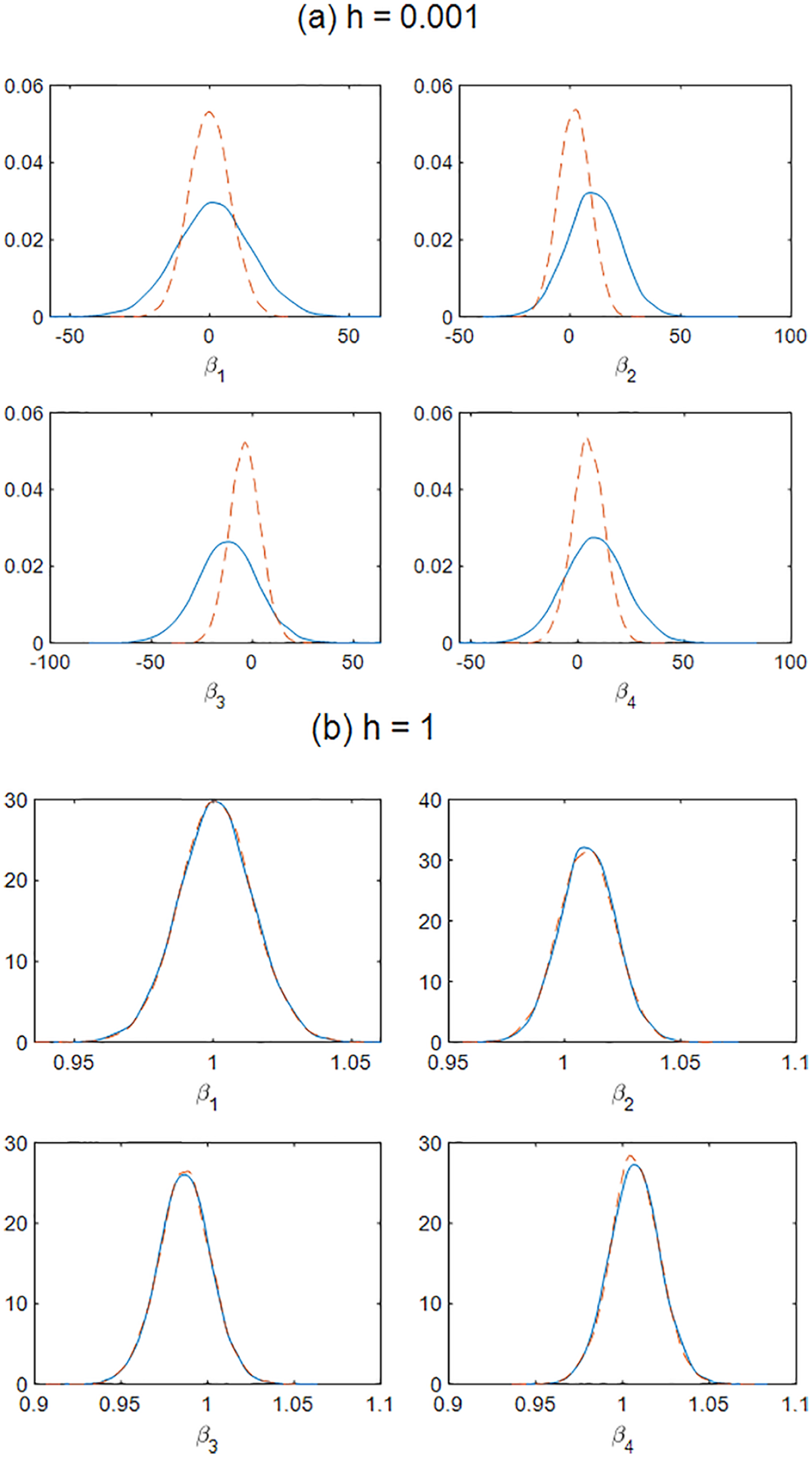
From these expressions it is clear that the informative prior (Equation 4) acts pretty much like ridge regression, while the flat prior (Equation 3) acts like OLS. As mentioned, we study the difference between the marginal posteriors under extreme collinearity ( $h = 0.001$ ) and less extreme or no collinearity at all ( $h = 1$ and $h = 10$ ).

Certain marginal posteriors are reported in Figure 1. Evidently, the marginal posteriors are quite different under extreme collinearity (Panel a), but the differences disappear in Panel (b) in which we used $h = 1$ . This is a case of nonharmful collinearity as, despite the fact that we have a maximal correlation coefficient between the explanatory variables close to 0.70, the marginal posterior densities are very close when we use the prior Equation 3 instead of Equation 4.

Figure 1

Marginal Posterior Densities

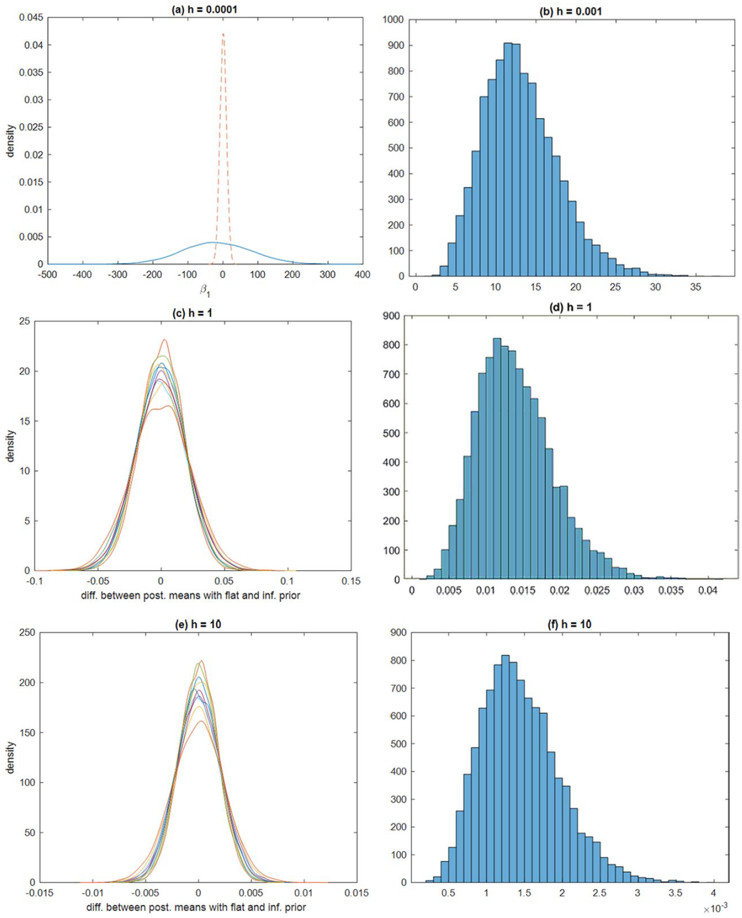
Marginal posteriors of the difference between the posteriors are reported in Panels (a), (c), and (e) of Figure 2. In Panels (b), (d), and (f), we reported median absolute differences between the two posterior means across all Markov Chain Monte Carlo draws. We used a Gibbs sampler with 15,000 passes and omitted the first 5,000 to remove the impact of possible start-up effects.

Figure 2

Marginal Posterior Densities of Differences of Parameters $β$ ( $n = 50, K = 10$ )

An important question is whether, besides visual inspection of posterior distributions, it is possible to deliver a single measure that can inform the user about the possibility of harmful collinearity. In the case of Panel (a) of Figure 1, we have applied the Kolmogorov–Smirnov test as to whether the univariate marginal posteriors corresponding to Equations 3 and 4 are the same. The p value of the test was zero, indicating rejection of the null that the univariate marginal posteriors are the same. In the case of Panel (b) the Kolmogorov–Smirnov test does not reject the null and the minimum p value (which can be employed more generally as a harmful collinearity test) was .0153. Finally, when $h = 10$ the minimum p value was .08. For the larger samples, the minimum p values of the tests were approximately the same. As it is known that the Kolmogorov–Smirnov test is very conservative, these results indicate that the marginal posteriors are definitely not the same when $h = 0.001,$ but this is not so for $h = 1$ or $h = 10$ .

The differences between parameters corresponding to the flat and informative priors in Figure 2 are more pronounced under extreme collinearity (Panels a and b) but tend to become smaller in moderate and absent collinearity (Panels c-f).

This is especially true of Panels (b), (d), and (f), which can be particularly useful for empirical researchers. So, the practical outcome is that harmful collinearity can be diagnosed by formal Bayesian analysis and histograms of median differences (as in Panels b, d, and f). More details and further results are provided in the appendix.

Hospitality Application

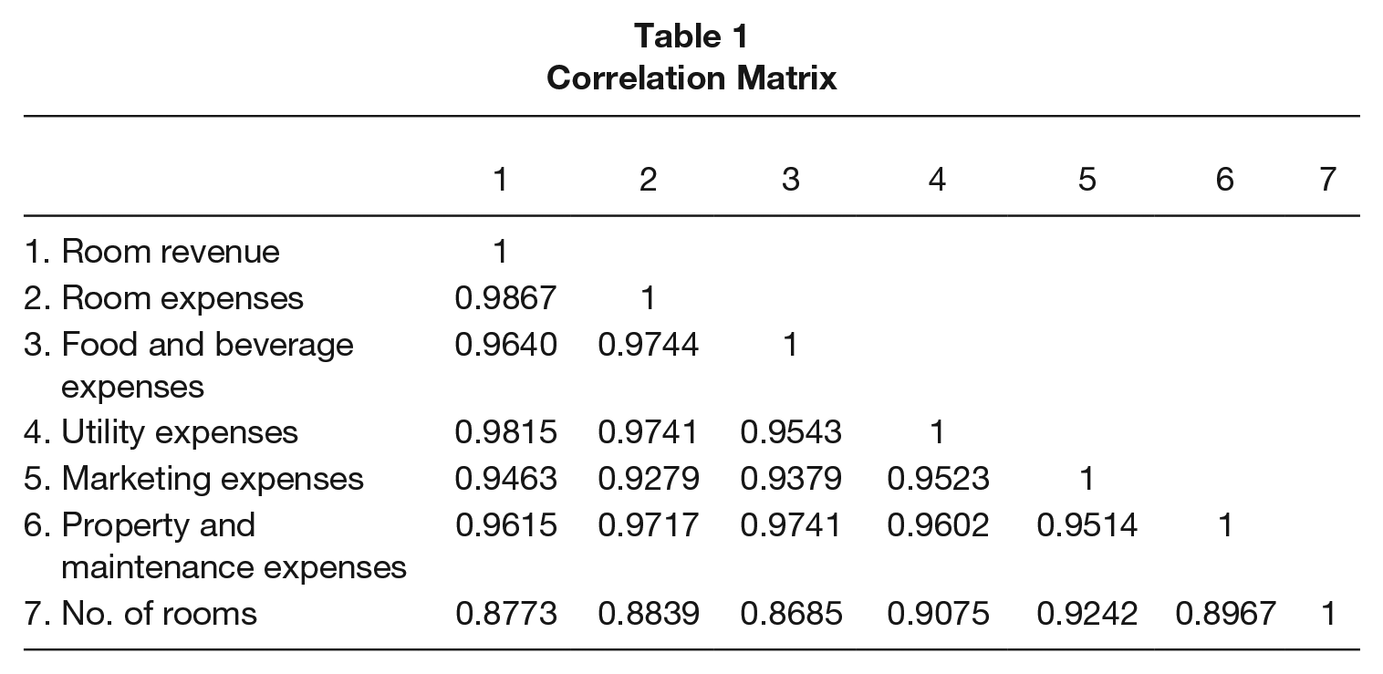
We also present an illustration of our proposed approach using an application on U.S. hotels. This regression focuses on the relationship between room revenue and the following covariates: room expenses, food and beverage expenses, utility expenses, marketing expenses, property and maintenance expenses, and number of rooms. We obtained all data from Smith Travel Research. The sample consists of 78 U.S. hotels (for the years 2012-2016) for a total of 390 observations. The correlation matrix for all variables included in the model (Table 1) clearly illustrates a high collinearity problem. Due to this, we expect the marginal posterior under OLS and the ridge-type prior to illustrate importance differences.

Table 1

Correlation Matrix

	1	2	3	4	5	6	7
1. Room revenue	1
2. Room expenses	0.9867	1
3. Food and beverage expenses	0.9640	0.9744	1
4. Utility expenses	0.9815	0.9741	0.9543	1
5. Marketing expenses	0.9463	0.9279	0.9379	0.9523	1
6. Property and maintenance expenses	0.9615	0.9717	0.9741	0.9602	0.9514	1
7. No. of rooms	0.8773	0.8839	0.8685	0.9075	0.9242	0.8967	1

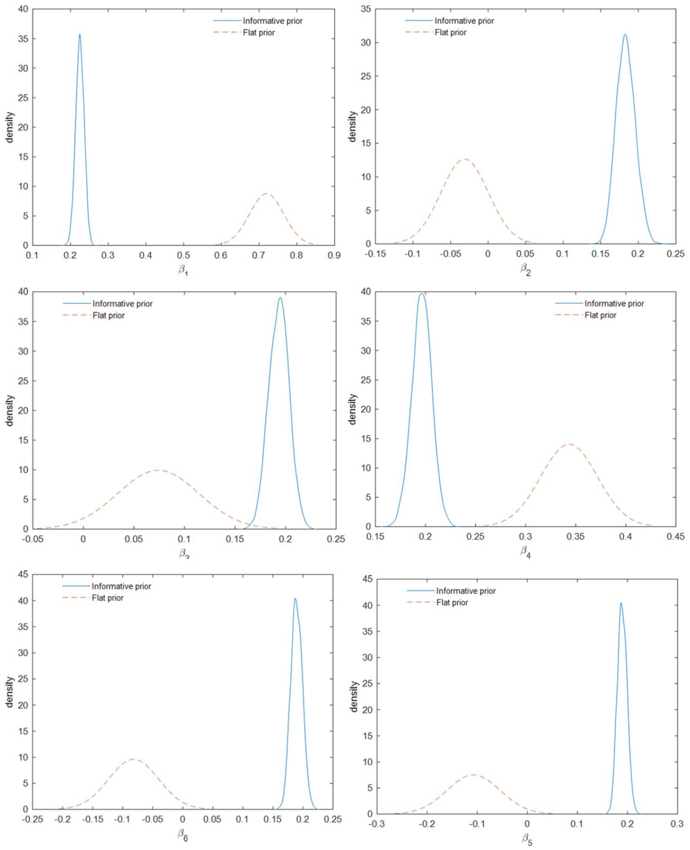
The results for the regressors we have in our models are presented in Figure 3. As expected, the difference between the flat and informative priors are pronounced, indicating multicollinearity problems. The two priors have even resulted in different signs for some of the coefficients. We have also applied the Kolmogorov–Smirnov test as to whether the univariate marginal posteriors are the same. The p value of the test was less than .01 for all coefficients, indicating rejection of the null that the univariate marginal posteriors are the same.

Figure 3

Marginal Posterior Densities of Parameters Under Informative and Flat Priors

Concluding Remarks

The Bayesian approach continues to grow in popularity in tourism research. In this article, we exploited the advantages this approach allows in testing for collinearity in tourism research. As one can directly observe the marginal posterior of regression parameters under the Bayesian approach, we recommend comparing this marginal posterior under the two priors. We showed that these two converge under nonharmful collinearity, but are substantially different under harmful collinearity. Along with direct visible inspection, we also recommend the use of the Kolmogorov–Smirnov test to confirm whether the difference between the marginal posteriors are significant.

Footnotes

Appendix

In Figure A1, we report the same posteriors as in Figure 1 with the only exception that $n = 1, 000$ and $K = 50$ .

Finally, we report, in Figure A2, the spectral measure

(7)

S = \frac{λ_{m i n}}{λ_{m a x}},

namely, the ratio of the minimum to the maximum eigenvalue of the cross-products matrix $X^{'} X$ . We assume $n = 100$ and $K = 10$ . In the case of extreme collinearity, the spectral measure is close to zero and, for this particular configuration of $n$ and $K,$ it ranges from about 0.2 to 0.47.

ORCID iD

A. George Assaf

A. George Assaf, PhD (corresponding author; e-mail: assaf@isenberg.umass.edu), is a professor and Hadelman family faculty fellow at the Isenberg School of Management, University of Massachusetts–Amherst. Mike G. Tsionas, PhD (e-mail: m.tsionas@montpellier-bs.com), is a professor at Lancaster University and Montpellier Business School.

References

Assaf

A. G.

Atkinson

S. E.

Tsionas

M. G.

(2020). Endogeneity in multiple output production: Evidence from the US hotel industry. Tourism Management, 80, Article 104124. https://doi.org/10.1016/j.tourman.2020.104124

Assaf

A. G.

Tsionas

M. G.

(2019). Forecasting occupancy rate with Bayesian compression methods. Annals of Tourism Research, 75, 439-449. https://doi.org/10.1016/j.annals.2018.12.009

Assaf

A. G.

Tsionas

(2020). Bayesian hypothesis testing for hospitality and tourism research. Journal of Hospitality & Tourism Research. Advance online publication. https://doi.org/10.1177/1096348020947327

Assaf

A. G.

Tsionas

Tasiopoulos

(2019). Diagnosing and correcting the effects of multicollinearity: Bayesian implications of ridge regression. Tourism Management, 71, 1-8. https://doi.org/10.1016/j.tourman.2018.09.008

Dogru

Sirakaya-Turk

Crouch

G. I.

(2017). Remodeling international tourism demand: Old theory and new evidence. Tourism Management, 60, 47-55. https://doi.org/10.1016/j.tourman.2016.11.010

Kalnins

(2018). Multicollinearity: How common factors cause Type 1 errors in multivariate regression. Strategic Management Journal, 39(8), 2362-2385. https://doi.org/10.1002/smj.2783

Morley

C. L.

(2009). Dynamics in the specification of tourism demand models. Tourism Economics, 15(1), 23-39. https://doi.org/10.5367/000000009787536654

Olya

H. G.

Mehran

(2017). Modelling tourism expenditure using complexity theory. Journal of Business Research, 75, 147-158. https://doi.org/10.1016/j.jbusres.2017.02.015

Tsionas

M. G.

Assaf

A. G.

(2020). Compression in stochastic frontier models. Annals of Tourism Research. Advance online publication. https://doi.org/10.1016/j.annals.2020.103026