Quantity or Spatial Coverage? Using Interpretable Machine Learning to Evaluate the Relationship Between Spatial Strategy of Police Stops and Crime in Crime Hotspots and Non-Hotspots

Abstract

As a result of variations in offender activity patterns in crime hotspots and non-hotspots, the spatial strategies of policing (such as the quantity and spatial coverage) should differ. Existing literature has not examined the spatially heterogeneous effect of police stop strategies on crime. This study focuses on the police stops-crime nexus in China, using the case of a major city’s central district. We introduce the spatial dimension of police stops—spatial coverage—in addition to the commonly considered quantity of police stops. Our results indicate that the spatial coverage of police stops surpasses the number of police stops as the most important crime predictor. We further find spatial heterogeneity in the police stop-crime nexus. A larger amount of police stops and spatially focused stops are more effective in crime hotspots. In crime non-hotspots, higher spatial coverage of police is more important in deterring crime than a larger number of police stops.

Keywords

crime police stops spatial strategy interpretable machine learning models

Introduction

Crime is likely to occur when motivated offenders, potential victims, and capable guardianship converge in time and space (Cohen & Felson, 1979). The rational choice theory predicts that motivated offenders evaluate potential benefits, risks, and costs in their criminal decision making (Cornish & Clarke, 2014). Police activities, such as patrols and stops, are a significant source of risk for potential offenders and shape their perception of risk, which, in turn, is directly linked to the likelihood of them acting upon their criminal motivations (Nixon & Barnes, 2019; Pogarsky & Loughran, 2016). Determining the optimal level and form of police activity is essential for effective crime deterrence.

However, literature on the crime deterrent effects of policing is still limited. Prior studies have paid much attention to police patrol experiments, while only a few studies have explored the relationship between daily patrol and crime at scale. Recent years have seen growing scholarly interest in using actual policing data to examine the impact of police stops on crime dynamics, particularly in the context of proactive policing strategies. The debate centers on whether increased police stops directly lead to a reduction in criminal activities or if the effect is more nuanced and contingent on spatial and temporal factors. This study examines this complex relationship in the context of China, where proactive policing practices are increasingly employed to address crime.

While the literature has noted the high concentration of crime in space, with certain areas disproportionately subject to crime (i.e., hotspots) (Andresen & Malleson, 2011; Crow & Bull, 1975; Weisburd, 2015), little is known about the effects of different spatial strategies of policing. Making offenders aware of police presence is crucial for crime deterrence. The frequency of criminal activities varies between hotspots and non-hotspots. The probability of police encountering potential offenders during patrols also varies across space. It follows that the spatial strategy for crime hotspots and non-hotspots should differ. The quantity and spatial coverage of police patrol are two key aspects of policing efforts against crime. But how these two aspects of police stops influence crime and how their impact varies across crime hotspots and non-hotpots remain underexplored. This study aims to fill this gap by pioneering an investigation into the spatial relationship between police stops and crime in China.

Comparison of Police Stops in China and the United States

Research on policing in China remains limited. Below, we briefly compare police stops in China with those in the United States, where the majority of policing studies are concentrated. Although police stops are an essential component of proactive policing in both countries, the processes and legal frameworks differ significantly. In China, the People’s Police Law (Article 9) grants police officers the authority to stop and question individuals in public spaces if they suspect a violation of the law. Officers are required to present their official identification before initiating a stop, and questioning is typically conducted by at least two officers. Stops are commonly triggered by observations of suspicious behaviors, appearances, or items. These stops target pedestrians and aim to maintain public security.

In the United States, stop, question, and frisk procedures are established by the Terry v. Ohio (1968) Supreme Court decision, which permits police officers to stop and detain individuals based on reasonable suspicion that a crime is being or will be committed. Reasonable suspicion requires specific, observable facts or behaviors that, based on the officer’s experience, suggest criminal activity. U.S. legal standards require a higher threshold for initiating a stop compared to China. The legal criteria in the U.S. are stricter, placing limits on police discretion and offering more protections for individual rights compared to China’s broader stop powers. Furthermore, in the U.S., stop, question, and frisk procedures are characterized by pronounced racial heterogeneity and generally elicit lower levels of citizen cooperation (Bradford, 2017; White & Fradella, 2016). In contrast, in China, there is a high degree of compliance with the police (Liu & Liu, 2018), resulting in greater cooperation during police stops.

Everyday Police Stops and Its Crime Deterrent Effects

In recent years, scholars have begun to use everyday police stop data to analyze the impact of police stops on crime, which contains information about the exact time and location of the behavior. Most studies show a significant negative correlation between police stops and crime. Using Poisson regression modeling, MacDonald et al. (2016) compare crime before and after an intervention and find that robbery and burglary rates decrease significantly as police stops increase in the study area. Using 2009-2010 New York City reported police stop data, Weisburd et al. (2016) use Bartik’s instrumental variable method and find that police stops have a significant deterrent effect on crime: as police stops in the study unit increases, the number of crime decreases.

On the other hand, some studies indicate that the impact of police stops on crime is not always significant. For example, Smith and Purtell (2008) observe differences in the impact of police stops on crime, and the impact varies by crime types. Their research shows statistically significant and negative effects of the lagged stop rates on rates of robbery, burglary, motor vehicle theft, and homicide but no significant effects on rates of assault, rape, or grand larceny. Rosenfeld and Fornango (2014) further use Arellano-Bond linear panel models to analyze the impact of police stops on two types of crime, robbery and burglary, for the period 2003–2020 in New York City. They find no significant effects of police stops robbery and burglary rates, with the exception of a small, marginally significant, negative effect of police stops on burglary rate after two years.

These inconsistent results can be due to such studies only concern the general spatial effects of everyday police stops on crimes. Everyday police stops likely have different effects on crimes in crime hotspots compared to areas with few crimes. Piza and Gilchrist (2018) find that police stops are typically concentrated near facilities that attract crime activities such as shopping malls and train stations, and the impact of police patrol and stops on crime varies by the surrounding environment. Despite evidence of the spatial heterogeneity in the police stops-crime nexus, no research has explicitly examined this heterogeneity.

Hotspot Policing

Crime hotspots are small areas with concentrated crimes. Hotspot policing—deploying police resources disproportionately in such high-crime areas—is considered an effective strategy to deter crime. Researchers have conducted foot patrol experiments in a number of cities, from the Kansas City Preventative Patrol Experiment (Kelling et al., 1974) and the Newark Foot Patrol Experiment (Kelling et al., 1981), to the Philadelphia Policing Tactics Experiment (Groff et al., 2015). They have found that hotspot policing can be more effective in suppressing crime and improving the efficiency of police utilization (Braga & Schnell, 2017; Durlauf & Nagin, 2011; Nagin et al., 2015; Taylor et al., 2011).

Theoretically, the effectiveness of policing is influenced by the level of offender activity (Parkinson, 2011), as frequent activity of offenders in crime hotspots increases the likelihood of police-offender encounters. According to the routine activities approach by Cohen and Felson (1979), effective guardianship is a pivotal element in disrupting the convergence of a motivated perpetrator and a suitable victim. This means that police stop behavior can only deter crime if the would-be offender perceives a meaningfully high probability of police-offender encounter. Offenders are often more active in crime hotspot than in non-hotspot, leading to differences in the probability of their encounters with the police. In this sense, in crime hotspots, the police are able to improve the probability of encounter with potential offenders through their daily patrols.

Moreover, it is important to note that crimes in hotspots can have different spatial-temporal features which will in turn impact police strategies. Ratcliffe (2004) proposes a hotspot matrix by dividing crime hotspots into different categories based on their spatial (i.e., dispersed, clustered, and hotpoint) and temporal (i.e., diffused, focused, and acute) characteristics and suggests varied prevention and detection strategy for each category. Furthermore, crime hotspots and non-hotspots may change with time. Crime hotspots may become non-hotspots during certain time and vice versa. This is especially true when considering weekly and seasonal rhythms of crime. However, hotspot policing experiments are limited by their static design—using fixed intervention areas and resource allocations—which makes it difficult to investigate the effectiveness of policing with the constant shifting of crime hotspots and non-hotspots. This also means that the prevention and control of crime non-hotspots should not be neglected and police should take efforts to prevent them from becoming crime hotspots.

Spatial Strategy of Policing: Quantity or Spatial Coverage of Police Stops

Different spatial strategies of policing shape the likelihood of police-offender encounter which will affect the effectiveness of police stops in deterring crimes. The relative benefits of intensive (i.e., increasing the quantity of police stops in specific hotspot locations) and extensive (i.e., spreading policing efforts to maximize coverage) policing remain understudied in the literature.

For the former, literature has found that both police stops and crime are spatially concentrated. For example, in a study of police stops in New York, Weisburd et al. (2016) found that 5% of street segments generated 77% of police stops, with 50% of these further concentrated at intersections. However, if police stops are targeted, although targeting police stops reduces crime in the hot area of intervention, it may lead to a shift of crime to areas that are not intervened (Bowers & Johnson, 2003). For the latter, increasing the rate of police visibility has always been an important means for the police to combat crime (Rosenbaum & Lurigio, 1994). Deterrence theory posits that perceived apprehension risk mediates the crime-prevention effect of police visibility. Intensive stops amplify this signal locally, whereas extensive patrols broadcast it widely. Durlauf and Nagin (2011) demonstrate that enhancing police visibility—either through hiring additional officers or strategically redeploying existing personnel to amplify the perceived risk of apprehension—consistently generates significant marginal deterrent effects on crime. In practice, the most direct way is to expand the coverage of police stops to cover as much of the precinct area as possible. While Weisburd et al. (2024) found crime reduction in large areas through dosage escalation, their analysis focused on large administrative units (e.g., police beats, precincts, or entire jurisdictions). This approach is conducive to increasing the deterrent range of police stops but often requires more police and material resources, making it hard and costly to implement. Moreover, the lack of focus in extensive police stops may lead to a decrease in the overall effectiveness of the intervention.

With a focus on the quantity of police stops, existing literature has so far paid limited attention to the spatial distribution of police stops, such as the spatial coverage. Only part of the literature has addressed the impact of police stops on crime from a spatial distribution or the size of area perspective. However, Schnell and Boehme (2024) applied Gini coefficients to quantify the spatial distribution of police stops, revealing no significant correlation between crime rates and stop concentration. As we have discussed earlier, the spatial aspect is crucial considering the spatial heterogeneity of crime concentration, the transition between crime hotspots and non-hotspots, and the potential displacement effect. For a given police precinct, how large an area of the precinct should be covered by patrols in order to achieve best results? It is not clear from existing evidence if covering a larger area leads to better patrol results. In addition, it remains unclear whether police stops strategies (both the quantity and their spatial coverage) may also show spatial heterogeneity across space (e.g., hotspots or non-hotspots).

Summary

In conclusion, existing literature has generally found that police stops have a certain but unstable negative effects on crime. There are three limitations in the literature. First, existing literature has not examined the spatial heterogeneous effect of police stops on crime, such as hotspot/non-hotspot areas. Second, most studies were carried out in American cities, New York City in particular. Third, research based on police foot patrol experiments, with its exclusive focus on crime hotspots, does not acknowledge the constant transformations between crime hotspots and non-hotspots. In so doing, existing studies do not offer a holistic understanding at the city scale and across time. Last, literature has only considered the quantity of police stops, but neglects the role of spatial coverage of police stops.

Therefore, this study explores the spatio-temporal distribution of police stops and its correlation with different policing strategies: the quantity of police stops and the spatial coverage of police stops. We further differentiate between crime hotspots and non-hotspots. The distinction between such areas is helpful for formulating more effective policing strategies. This study pioneers the investigation of the spatial relationship between police stops and crime in China. It offers new insights into our understanding of the “offender-victim-police” spatial-temporal interactions by introducing spatial heterogeneity in policing strategies in a non-Western context.

Data and Methods

Study Area and Study Units

This study focuses on the central district of ZG city¹, one of the mega cities in South China. In 2019, the central district led the city in economic output, with a per capita GDP of 285,200 RMB. The central district covers over 100 square kilometers and is home over 2 million residents, among whom 1.09 million are registered as local residents. The area is characterized by dense mid- to high-rise buildings and predominantly flat terrain, with plains accounting for 63.34% of its landscape.

Regarding the unit of analysis, studies on police stops and crime have used both small (e.g., grids and streets) and large spatial units (e.g., neighborhoods, police stations) (Rosenfeld & Fornango, 2014, 2017; Weisburd et al., 2016). Small units are preferable for capturing the actual environment that sets the stage for human behaviors including the interactions between motivated offenders, potential victims and guardianship. Grids are a commonly used analytical unit in crime research (Song et al., 2018). This paper uses 500 m × 500 m grids as the unit of analysis. According to the existing urban road planning and design specifications in China, the spacing of branch roads ranges between 500 m and 600 m. The 500 m grid size thus aligns with typical urban road patterns. There are a total of 619 grids within the study area. The analysis delves into the police stop-crime relationship on a weekly basis throughout the year 2019. This gives us a sample size of 32,188 (619 × 52 = 32,188) grid-weeks for the machine learning models.

Research Data

The dependent variable for this study is binary: whether or not there was street crime during the current week in the grid cell (yes: 1, no: 0). Street crime includes street thefts, robberies and assaults, accounting for 49.88% of all crimes in 2019 in the study area. Our crime data consists of verified reports, with each incident confirmed by an officer on-site to ensure that only actual crimes are recorded in the system. These data consist of 110 emergency call records during December 24, 2018 and December 31, 2019 provided by the ZG City Public Security Bureau. The data includes details of the type, geographic coordinates, and time of each crime. Out of all 32,188 grid-weeks, 76.16% had no crime during the study period, and 14.82% had only 1 crime. Following Zhang et al. (2022), all grids with crime are considered hotspots, and these study focus on whether a crime occurs in a grid.

This study selects independent variables informed by routine activity theory and crime pattern theory. According to the routine activity theory, necessary conditions for crime to occur include potential offenders, suitable targets for crime, and the absence of capable guardianship. We approximate the presence of potential offenders based on the presence of crimes in the previous week, suitable targets by the neighborhood ambient population, and the absence of guardianship by variables related to police stops (i.e., quantity of police stops in the previous week and the coverage of police stops in the previous week).

Quantity and Spatial Coverage of Police Stops in the Previous Week

The police stop data from December 24, 2018 to December 31, 2019 are provided by the ZG City Public Security Bureau. We focus on police stops that are primarily conducted on pedestrians on the streets. Typical procedures of stops involve temporarily and non-intrusively detaining or restricting their freedom of movement if they are suspected of potential criminal behavior. Pedestrians stopped by the police are required to present their ID cards or provide their ID numbers for identity verification. Police officers use dedicated smartphone devices during stops. These devices allow officers to access individuals’ personal information including gender, age, and criminal history, while automatically logging the timestamp and location of the stop. This setup not only streamlines police work but also minimizes the risk of manual input errors. Data without a valid timestamp or geographic coordinates (mainly due to technical problems with the device) are dropped, accounting for 29.4% of all police stop records. During a police encounter, if the device has no signal or the police cannot identify the target person’s ID card, the police will make several attempts until they succeed. In other words, the missingness does not affect the accurate measurement of the number of police stops.

The quantity of police stops and the coverage of police stops are two key indicators of police patrol behaviors. To measure the coverage of police stops, we merge the buffer zones around each police stop location (radius = 10m) and calculate the ratio of total buffer zone area to the grid area. The variables are calculated for each grid-week. Figure 1 shows an example of the difference between quantity and spatial coverage of police stops. Grid A has a total of 6.79 (standardized value) police stops with a spatial coverage of 20.8%. Note that due to the confidentiality agreement with local public security authority, the quantity of police stops was standardized in this study. Grid B has a quantity of 8.27 (standardized value) police stops, which is far larger than that of Grid A, while its spatial coverage reaches only 11.2%, smaller than that of Grid A. This example shows that large quantity of police stops in a grid does not necessarily also mean high spatial coverage rate. The correlation index between police stops and spatial coverage for all grids is 0.594 (p < .001).

Figure 1.

Standard deviation ellipse of police stops of partially grids.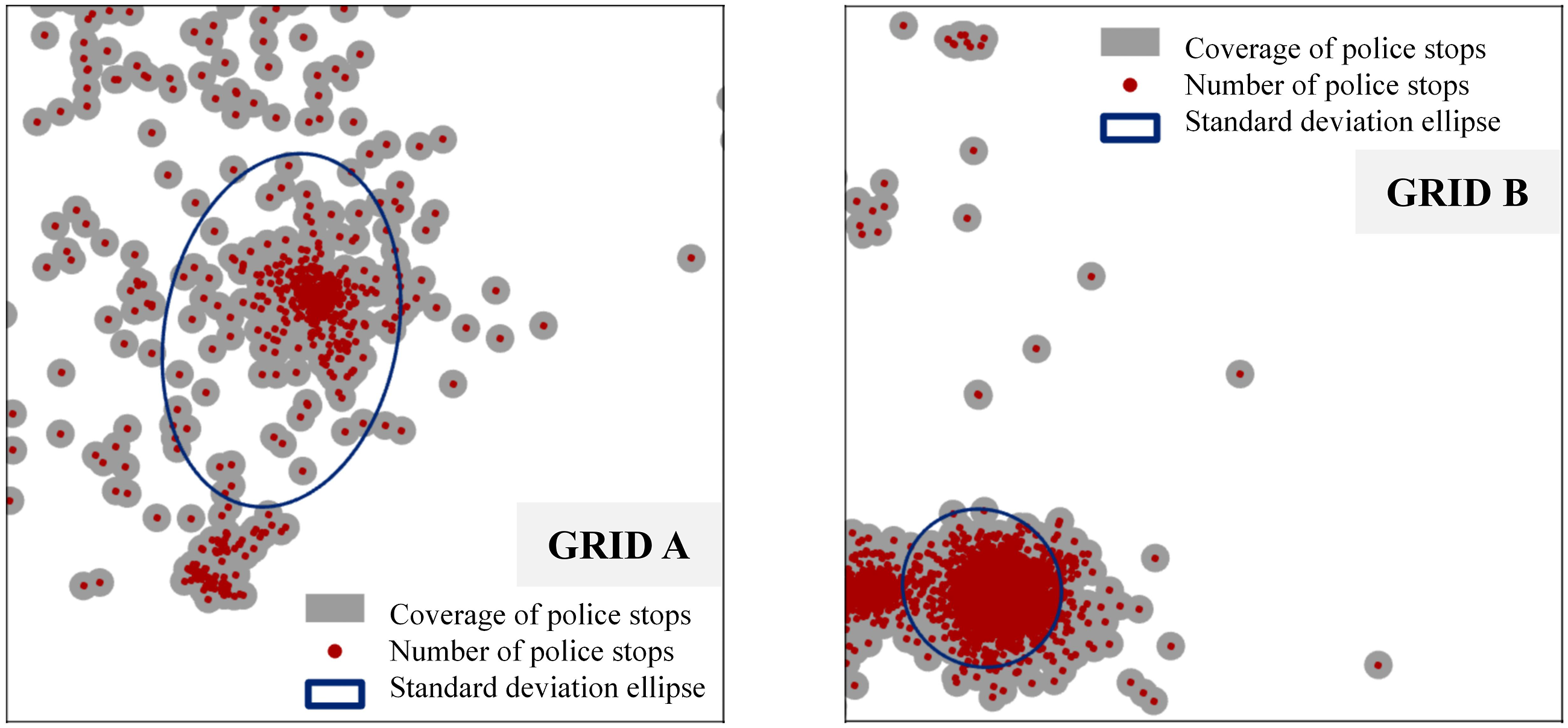

In Figure 2, we further plot the quantity of police stops (x-axis) against the coverage of police stops (y-axis) for 52 cycles of each grid. We find that when the quantity of police stops varies between 0 and approximately 7 units, the coverage of police stops also increases gradually, reaching a maximum of 35.49%. When the quantity of police stops exceeds 7 units, the coverage of police stops fluctuates around 15%. This suggests that the spatial coverage of police stops does not continue to increase with the quantity of police stops. Police stops are concentrated in small spatial areas when the quantity of police stops is increasing.

Figure 2.

Scatterplot of quantity of police stops and coverage of police stops.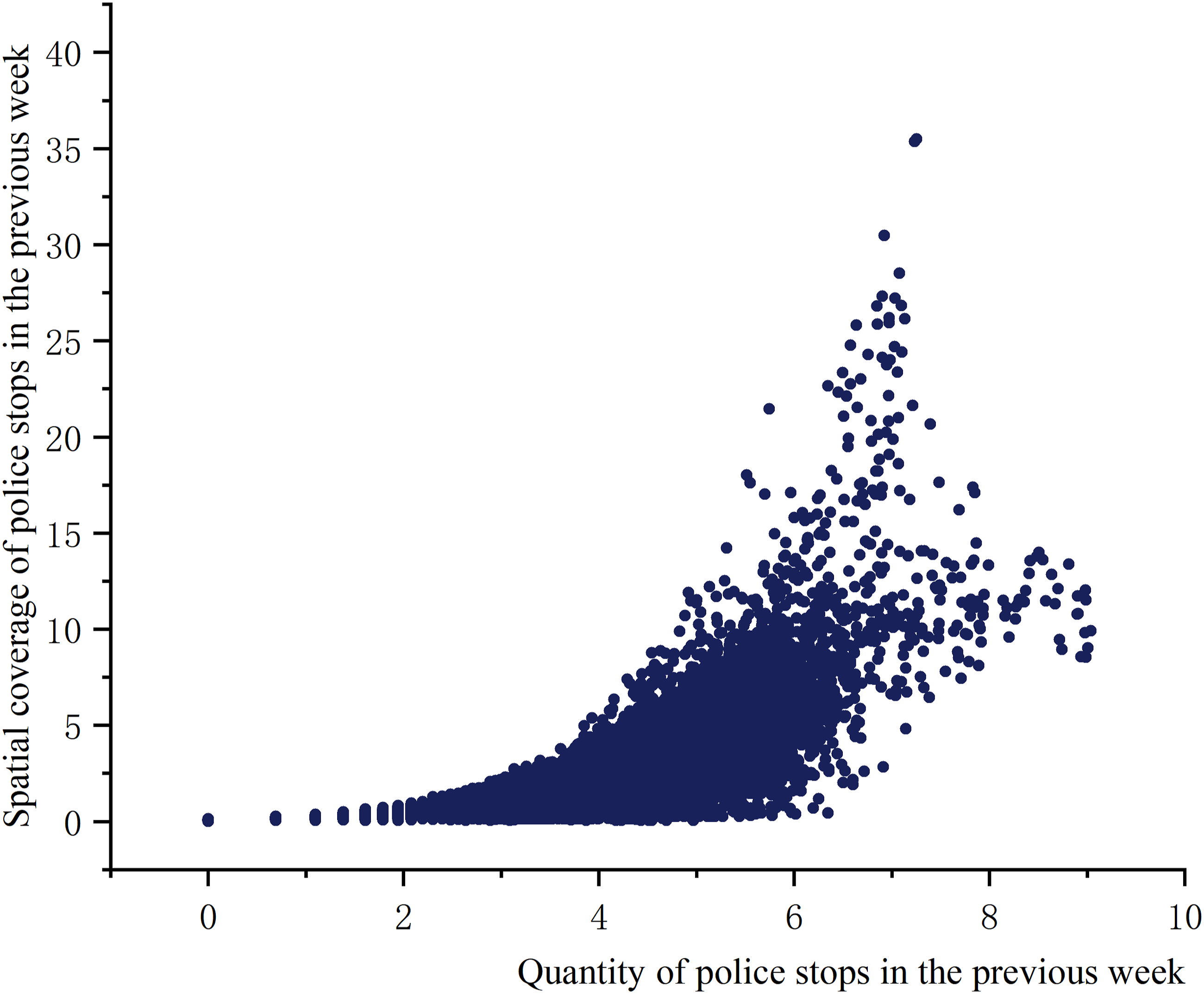

As the relationship between crime and police stop during the same week is reciprocal, it is hard to distinguish the sequence of crime and police stops in the same week. To address this issue, this study uses one-week-lagged police stops variables.

Street Crimes in the Previous Week in the Grid

Previous research suggests that the occurrence of crime is time-dependent (Haberman & Ratcliffe, 2012; Marchione & Johnson, 2013). Besides, it also can act as the indicator of the presence of potential offenders. Due to the sparsity of crime data, we operationalize historical crime as a binary variable with 1 representing at least one crime incident in the past week and 0 otherwise.

Ambient Population

Recent empirical work has demonstrated that the use of residential population alone is not a reliable measure of potential victims. Instead, ambient population, the total population present at certain space and time, emerges as a more accurate proxy (Malleson & Andresen, 2016). Previous research suggests that cell phone data offers a viable way to estimate ambient population (Gonzalez et al., 2008) and it can be used to analyze and predict the spatial and temporal patterns of crime (Song et al., 2023). In contrast, cell phone data captures all individuals present in an area, regardless of whether they are residents. The ambient population data used in this paper is derived from cell phone signal big data from China Unicom Inc, one of the three major carriers in China. The company accounts for 20.78% of China’s cellular carrier market share. The telecom company gathers user data through cellular base stations. When a user initiates active communication (e.g., making calls, texting, or making data usage), the device prompts the carrier to log the user’s location; when no active communication is detected, the carrier captures the user’s location every 30 minutes. The individual-level footprint data along with socio-demographic attributes are anonymized and aggregated to grid cells in the data platform Daas. It is rather hard to obtain this big data throughout a year. With reference to Zhang et al. (2022) (using data of one week to represent the population of a year) and Song et al. (2023) (using data from two days of a week to represent the population for weekday and weekend), the spatial distribution of population is relatively stable. Therefore, in this study, we use ambient population data of October 2019 to calculate statistics for grids in the study area to represent the ambient population.

Point of Interest (POI)

Crime pattern theory (Brantingham & Brantingham, 1993) emphasizes that crime is concentrated in places that are attractive to potential offenders, such as home, work or school, transportation nodes, shopping malls, parks and recreation centers, and the paths that connect these “cognitive spaces”. In this paper, following Brantingham and Brantingham (2017) and Song et al. (2019), we include the number of restaurants, bus stops, subway stations, department stores, internet cafes, entertainment venues, schools, banks, hotels, and convenience stores based on 2018 POI data for the city of ZG provided by a major map navigation company.

The descriptive statistics are shown in Table 1. The standardized number of police stops has a mean value of 1.619 standard units. On average, 0.238 of the grid-weeks experienced crime during the study period. We account for the right skewness in ambient population and POIs by adding 1 to the values and applying the natural logarithm.

Table 1.

Descriptive Statistics of Variables (N = 32,188).

Variable	Mean	Std. Dev	Min	Max
Presence of street crime in the previous week	0.238	0.426	0	1
Quantity of police stops in the previous week	1.619	1.944	0	9.04
Coverage of police stops in the previous week (%)	0.95	2.09	0	35.49
Ambient population	10.767	1.43	6.782	14.693
Bus station	0.643	0.721	0	2.833
Department store	0.701	0.904	0	3.784
Internet café	0.275	0.537	0	2.773
Entertainment venue	0.502	0.796	0	3.258
School	0.541	0.715	0	2.944
Hotel	0.703	0.959	0	4.078
Bank	0.718	1.034	0	3.892
Convenience store	0.364	0.625	0	2.708
Restaurant	1.384	1.501	0	6.426
Rail station	0.111	0.380	0	2.303

Methodology

Currently, some scholars have applied machine learning and SHAP interpreters to the prediction and explanation of crime (Alves et al., 2018; Kang & Kang, 2017). With SHAP interpreter, researchers can test the correlation between independent and dependent variables and the interaction effects between independent variables (Xiao et al., 2021; Yang et al., 2021) and visualize their spatial relationship (Li, 2022). For example, Kim and Lee (2023) use LightGBM model and reveal a nonlinear relationship between crime incidence and the urban environment. Zhang et al. (2022) find that XGBoost, a widely recognized machine learning tree model that can well balance accuracy, flexibility and efficiency (Mousa et al., 2018), outperforms other common machine learning models in crime prediction.

This study compares different popular machine learning models (e.g., Logistic Regression, Decision Tree, Random Forest, GradientBoosting and LightGBM) and reports the AUC value (area under the curve) of all the models. The larger the AUC value, the better the model performance. It can be seen that the XGBoost model clearly shows the best model fit (Figure 3). Thus, the present study uses the XGBoost model.

Figure 3.

Comparison of ROC curves of different models.

The XGBoost model classifies a given sample according to the decision rules in the tree model and predicts the scores in the cumulative classified leaves (Chen & Guestrin, 2016). A model with k decision trees takes the following form: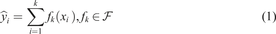

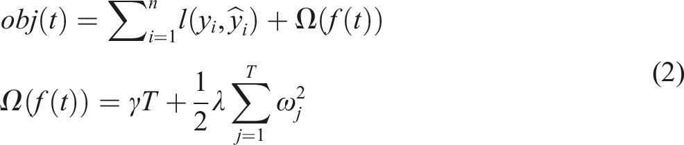
{\hat{y}}_{i} = \sum_{i = 1}^{k} f_{k} (x_{i}), f_{k} \in F

(1)

The objective function is as follows:

\begin{array}{l} o b j (t) = \sum_{i = 1}^{n} l (y_{i}, {\hat{y}}_{i}) + Ω (f (t)) \\ Ω (f (t)) = γ T + \frac{1}{2} λ \sum_{j = 1}^{T} ω_{j}^{2} \end{array}

(2)

In the equation (2), the

l (y_{i}, {\hat{y}}_{i})

is the target

y_{i}

and its prediction

{\hat{y}}_{i}

of the loss function.

Ω (f (t))

is the regular term of the objective function, which indicates the complexity of the whole tree.

γ

is the penalty coefficient that controls the number of leaf nodes to prevent overfitting,

λ

is the regularization coefficient,

T

is the total number of leaf nodes, and

ω_{j}

is the weight of leaf nodes. The total number of leaf nodes and the vector paradigm of weights together determine the size of the regularization term.

The model can compute the optimal solution of the entire model, balance between minimizing the loss function and the complexity of the model, and avoid overfitting while improving the efficiency of the model (Mousa et al., 2018). Furthermore, XGBoost has the advantage of incorporating all predictors into the model without incurring multicollinearity penalties (Parsa et al., 2020).

Shapley additive explanation (SHAP) is a game-theory-based approach to model explanation proposed by Kuhn and Tucker (1953). When applied to machine learning models, this method can help understand the process of indicator characterization, classification, and prediction. In addition, SHAP can explain the model at both global and local levels. A positive SHAP value indicates a positive impact of the variable on the model outcome, while a negative value indicates a negative effect. The SHAP Interaction value can be used to interpret the model by considering the interaction of the two features in global interpretation.

This paper explores the relationship between police stops and crime based on the trained XGBoost model using the SHAP method’s tree model interpreter (TreeExplainer). We encourage readers interested in the technical details of the methods to methodological papers such as Lundberg and Lee (2017) and Mousa et al. (2018).

The Spatial and Temporal Distribution of Police Stops and Crime

We plot the weekly quantity of crimes in the current week and the quantity of police stops in the previous week (Figure 4). First, the quantity of police stops and crime both fluctuate over time and the overall shapes are similar. The correlation between the two variables over 52 weeks is 0.36. Second, there are obvious troughs and peaks in both the quantity of police stops and the quantity of crimes. Third, while the overall trends of police stops and crimes over time are similar, most dips in the quantity of crimes correspond to peaks in police stops in the week before. For example, the quantity of crimes in the 14th week was at a trough, but the quantity of police stops in the previous week was at a peak.

Figure 4.

Weekly Changes in police stops and crime in 2019 (Max-min based normalization).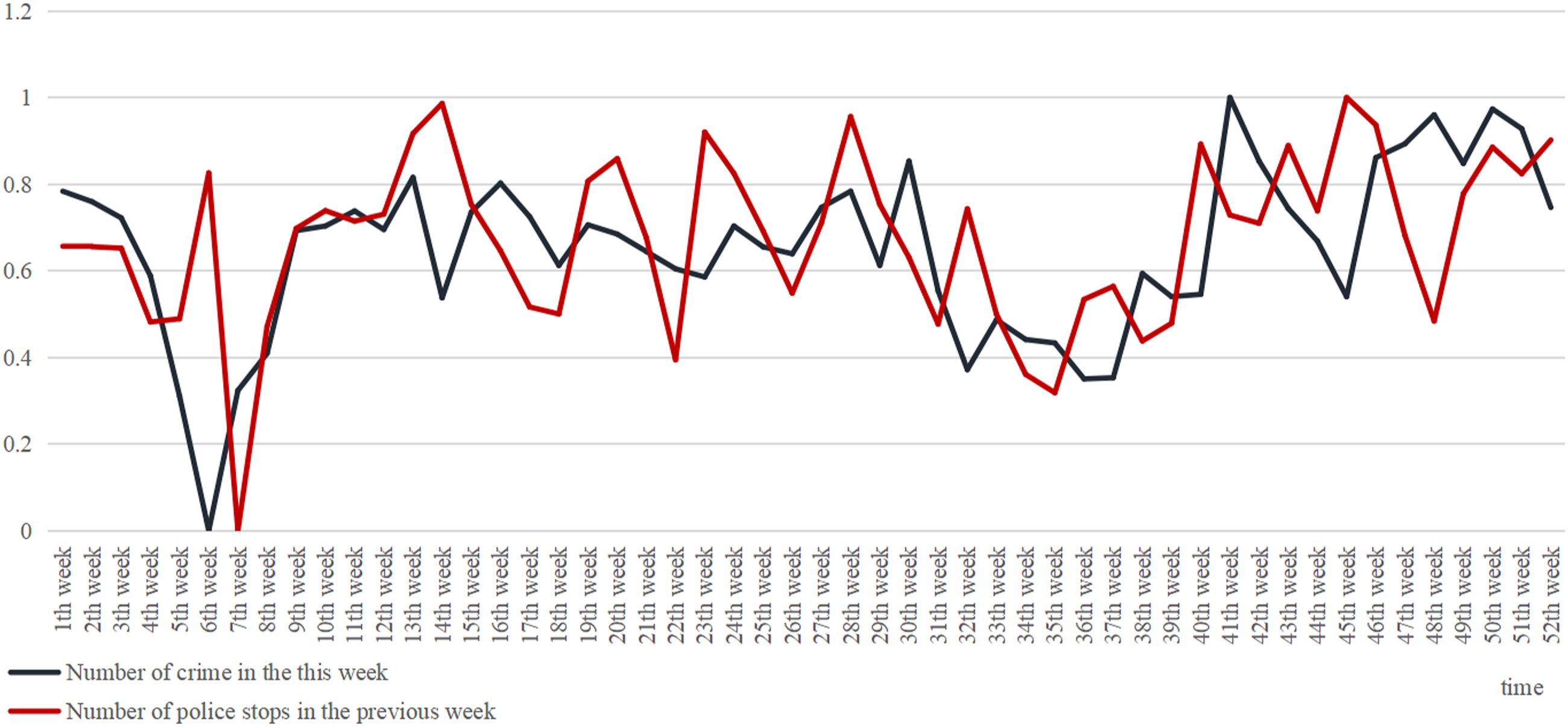

The spatial distributions of police stops and crimes (Figure 5) show that there are hotspots in both police stops and crime in space. At the grid level, there is some spatial similarity in the distribution of police stops and crime. Their shared hotspots are particularly concentrated in the upper part of the study area, where there is high population mobility and heterogeneity, such as commercial districts and urban villages. There is a clear consistency in the spatial distribution pattern of the quantity of police stops and the coverage of police stops.

Figure 5.

Spatial distribution of police stops and crime in 2019. Note: Due to the confidentiality agreement with the ZG Municipal Public Security Bureau, maps involving the study area have been encrypted, and it is not appropriate to add a compass and other map elements.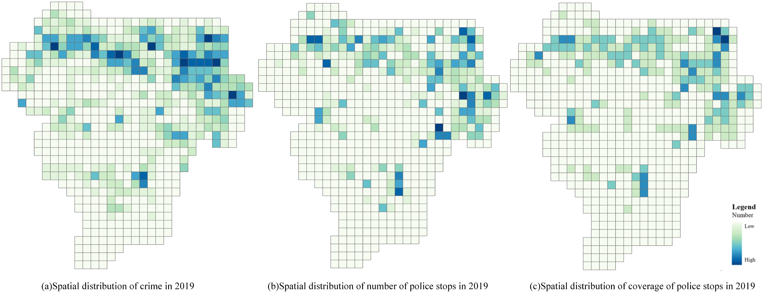

Model Results

XGBoost Model Results

This study uses XGBoost to model the binary classification of whether a street crime occurred in each grid-week. The dataset is randomly divided into a training set (75% of all samples) and a test set (25% of all samples). The parameters are tuned using the grid search method. We train the model by using different combinations of parameters and the performance of each combination is evaluated using ten-fold cross-validation to find the optimal combination.

The final results show an accuracy of 0.8712 in the training set and 0.8233 in the test set, meaning that 87.12% and 82.33% of the grids are predicted correctly in training and testing, respectively. According to the feature importance ranking results from XGBoost (Figure 6), the coverage of police stops in the previous week is the most important feature, followed by the quantity of police stops in the previous week and the ambient population. In contrast, POI of all kinds do not have as much impact on crime as police stops and population do.

Figure 6.

XGBoost model feature importance ranking.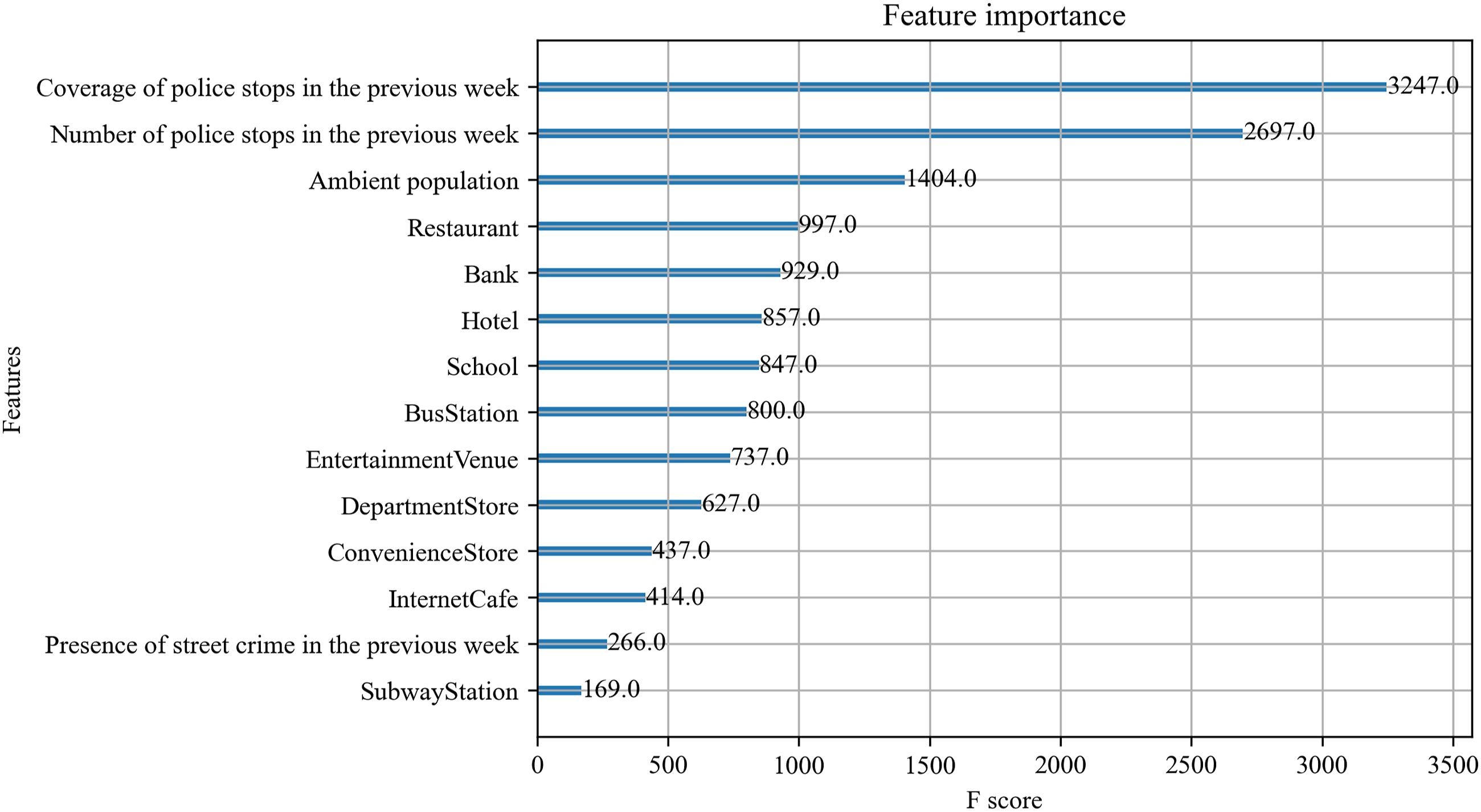

The Relationship Between the Quantity and Spatial Coverage of Police Stops and Crime

To further investigate the relationship between police stops and crime, we plotted the scatterplot of the number of police stops and the corresponding SHAP Values. The relationship between the quantity of police stops in the previous week and crimes in the current week is non-linear. Further calculation shows that the proportion of samples in which police stops had a negative impact on crime outcomes during the previous week is 60.59%, which indicates that the previous week police stops have an overall negative impact on the occurrence of crime during the week.

Specifically, when the quantity of police stops is between 0 and 2 standard units, the quantity of police stops is positively correlated with the occurrence of crime during the week. This is evidenced by the gradual increase in the corresponding SHAP values, i.e., the positive impact on the occurrence of crime during the week gradually increases. When the quantity of police stops in the previous week falls within the [2,6) range, similar to the previous interval, a higher count of police stops in the previous week positively predicts the occurrence of crime during the current week. However, the rate of increase in this positive effect is considerably lower. When the quantity of police stops in the previous week is in the [6,10) range, the relationship turns from positive to negative. The largest negative effect is observed when the quantity of police stops is around 7 standard units. After the value exceeds 8, the negative effect begins to diminish.

Next, we similarly plot the SHAP value scatterplot of coverage of police stops in the previous week (Figure 7(b)). The overall trend shows that the coverage of police stops and the corresponding SHAP value in the previous week show a fluctuating upward trend. By counting the positives and negatives of SHAP values, 59.45% of the sample has coverage of police stops negatively affecting the crime outcomes. When the coverage of police stops falls within the [0,5) interval, it has a negative influence on crimes, with 62.16% of SHAP values being negative. When it falls in the [5,15) interval, the influence of police stop’s spatial coverage begins to intensify, with negative impacts maximized at a spatial coverage close to 8 units. While falling in the in the [15,40) interval, the scatter points are all above the x-axis, representing an overall positive influence.

Figure 7.

SHAP values scatter plot of quantity/spatial coverage of police stops in the previous week.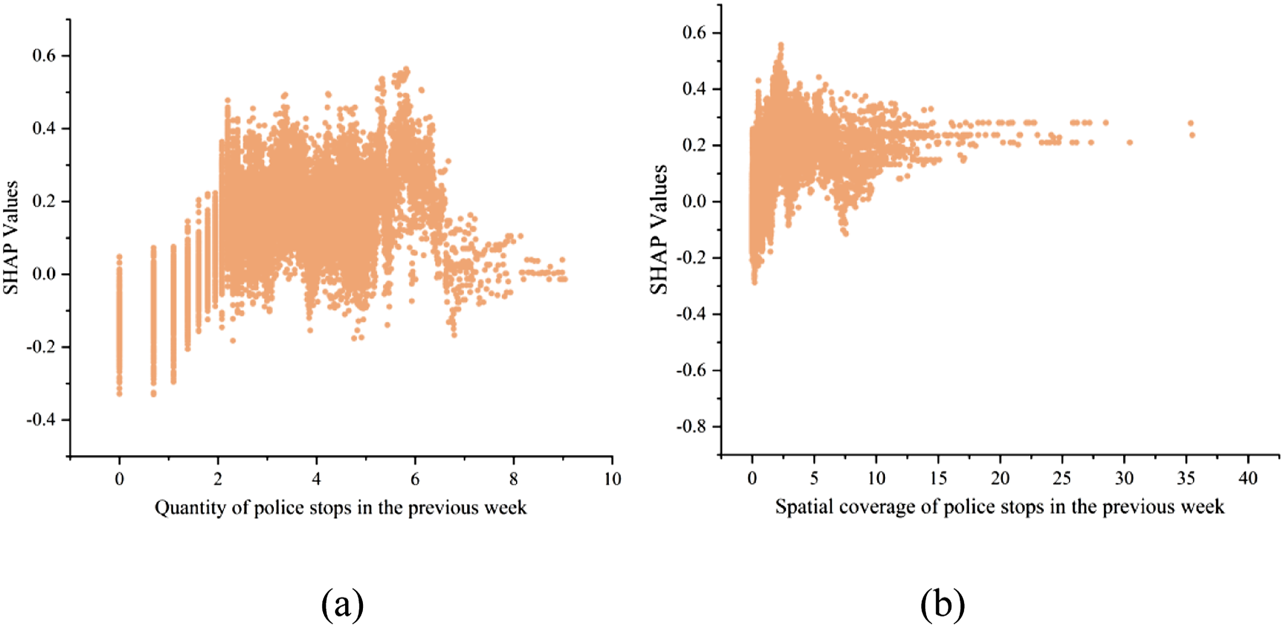

The Interaction Effects of Police Stops Quantity and Crime Hotspots as Well as Non-Hotspots

We then calculate the SHAP Interaction Values between the quantity of police stops in the previous week and whether a crime occurred in the current week. We further plot SHAP Interaction Values against the quantity of police stops for hotspot grids (crime occurred in the previous week) and non-hotspot grids (no crime occurred in the previous week) separately (Figure 8). As for non-hotspots, the quantity of police stops produces the strongest crime deterrent effect under the [2,5) interval. When the quantity of police stops exceeds 6, the dispersion of police force leads to an increase in the probability of crime.

Figure 8.

The quantity of police stops in the previous week against SHAP interaction values.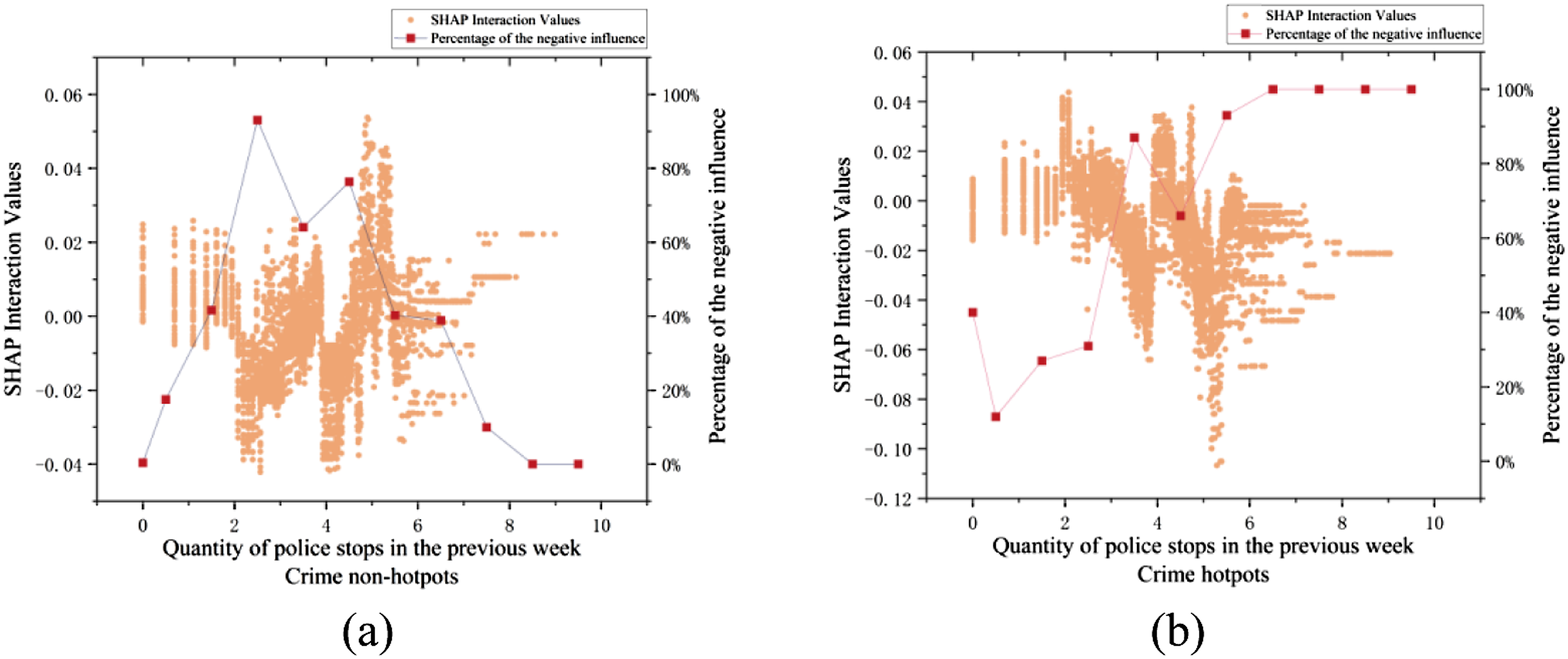

When it comes to police stops in hotspots, the SHAP Interaction values turns negative as the quantity of police stops increase, showing a roughly negative correlation. When the quantity of police stops in the previous week surpasses 3 standard unit in crime hotspots, the deterrent effect on crime in the current week becomes increasingly powerful. In particular, at a standard value of 6, the effect of police stops on crime is completely negative, showing strong deterrent effects on crimes.

The Interaction Effects of Police Stops Spatial Coverage and Crime Hotspots as Well as Non-Hotspots

We conduct similar analysis and visualization by interacting the spatial coverage of police stops and crime. For non-hotspot grids (Figure 9(a)), by increasing the coverage of police stops in the previous week, there is a significant negative effect on crime occurrence. This suggests that when police stops are conducted in non-hotspot areas, increasing the coverage can reasonably deter crime.

Figure 9.

The spatial coverage of police stops in the previous week against SHAP interaction values.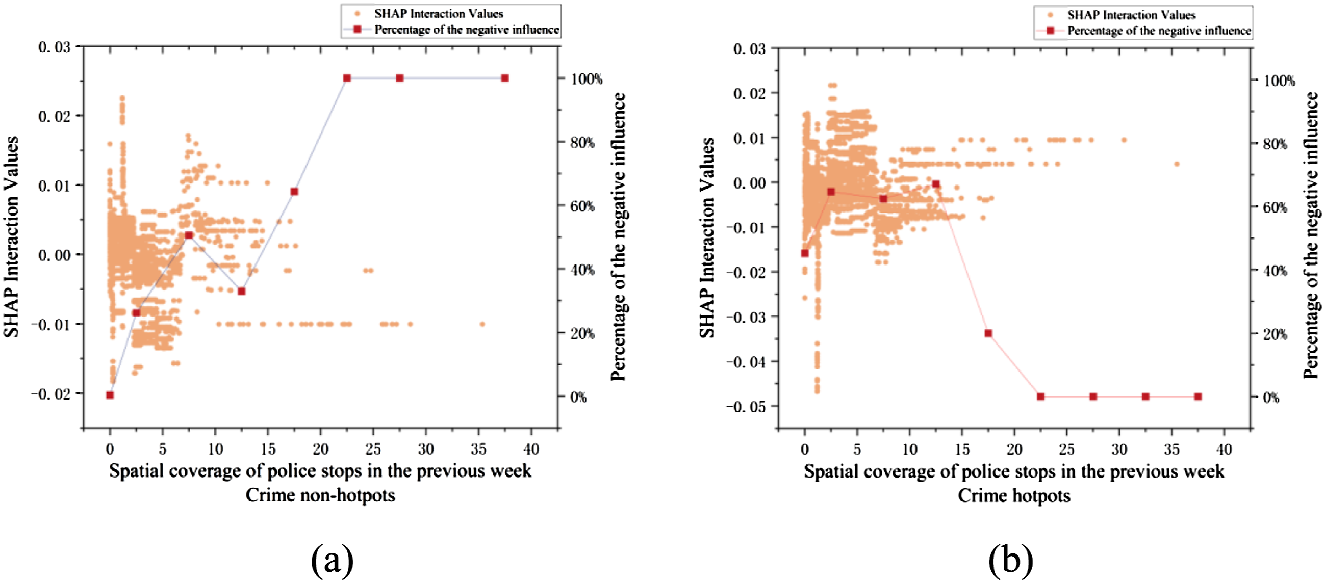

By contrast, for crime hotspot grids (Figure 9(b)), the deterrent effect on crime in the current week is significantly compromised by increasing the coverage of the previous week’s police stops. When the spatial coverage of police stops is small, there is a significant negative effect on crime occurrence. As the spatial coverage of police stops expands, the negative effect significantly diminishes and the share of grids in which the effect is negative decreases significantly, despite that most of the points still have a SHAP Interaction values below 0. It indicates that when police stops are conducted in hotspot areas, concentrated rather than dispersed police force is more effective in deterring crime. In Figure 9(b), the smallest SHAP interaction value is −0.047 when the spatial coverage of police stops reach 1%, with 70.91% values being negative (the corresponding number of police stop points is 8). It means that in a hotspot grid, conducting police stops at 8 locations, that are more than 10 meters apart from each other, can have sound deterrent effects on crimes.

Discussion

Making the offenders aware of the police presence is a fundamental prerequisite for the police to effectively dissuade criminal activities. It is noteworthy that behavioral patterns of offenders may vary significantly in crime hotspots and non-hotspots. The likelihood of police encountering potential offenders during patrols differs significantly across space, indicating that the spatial strategies of police stops (e.g., quantity and spatial coverage) in crime hotspots and crime non-hotspots should also vary. Furthermore, these crime hotspots are not static but evolve and shift over time. To this end, this study examines the spatial heterogeneity of the quantity and spatial coverage of police stops in crime hotspots and non-hotspots. To do so, we use an interpretable machine learning approach with weekly crime and police patrol data for 500 m grids in the central area of ZG city. As a key concern of this study, the importance of spatial coverage and quantity of police stops rank top among all the explanatory variables. Both have general deterrent effects on crime but further analyses suggest that such effects vary across spatial units.

As the quantity increases, police stops tend to be clustered in limited geographic space with small spatial coverage. Further, the quantity of police stops and the spatial coverage of police stops do not always produce inhibitory effect on crime. Specifically, the deterrence effect of the quantity of police reaches its maximum at 7 standard units. The negative effect of police stops on crime is more pronounced when the spatial coverage of police stops is less than 10 units.

The findings suggest that the number and spatial coverage of police stops do not necessarily correlate positively with a stronger suppression of crime. When devising policing strategies, official agencies may be inclined to double efforts to combat crime. However, merely increasing the quantity of police stops or the spatial coverage of police can not only lead to a waste of police resources but also fail to achieve the desired outcomes. While Weisburd et al. (2024) have demonstrated that increasing the dosage of stops can enhance crime prevention over larger areas, our empirical findings suggest that a higher number of stops does not necessarily mean broader spatial coverage. Instead, increased stop frequency often leads to more concentrated coverage, and such resource-intensive efforts do not always suppress crime. Consequently, it is advisable to maintain both the number of police stops and their spatial coverage within an appropriate range based on their deterrent effects on crimes.

Another related finding is that police stops produce different effects in crime hotspots and non-hotspots. For both crime hotspots and non-hotspots, a small number of police stops does not have a deterrent effect on crime. However, for hotspots, the optimal number of police stops is between 6 and 10 standard units for deterring crime, with limited marginal changes beyond 10 units. This would indicate that police stops exceeding this threshold are a waste of police resources in hotspots. For non-hotspots, high-intensity police stops may lead to an increase in crime instead. One explanation is that as the quantity of police stops grows, police stops become more routinized and concentrated spatially (see Figure 5). Moreover, regular police patrol will be easily anticipated by offenders, which in turn helps them avoid the risk of being captured, leading to a higher risk of crime occurrence (Barr & Pease, 1990).

Similarly, the effect of spatial coverage of police stops differs significantly for crime hotspots and non-hotspots. For crime non-hotspots, high spatial coverage is important, and the best deterrent effects are achieved at 20% spatial coverage. For crime hotspots, spatially concentrated police stops, i.e., a low spatial coverage, become more important for crime prevention. When spatial coverage increases in hotspots, the crime controlling effect of police stops decreases significantly. This can be due to the different activity patterns of potential offenders in these two kinds of areas. In crime hotspots, potential offenders would often engage in non-criminal routine activities through which they can build up their spatial awareness of crime opportunities (Brantingham & Brantingham, 1993), while acting upon any criminal opportunities as they emerge. When police patrols in crime hotspots, they are more likely to encounter potential criminals, which means even if the police only conduct police stops in specific locations with a small spatial coverage, it still serves as a deterrent to offenders. On the contrary, if the spatial coverage is too large, it often means that the quantity of police stops at a given point decreases. This can make offenders realize that the police are only stopping for a short time, and they may choose to wait for an opportunity to commit a crime in that area. In crime non-hotspots, the likelihood of offenders being active or committing a crime in that area is low (Nagin et al., 2015). For police, if their daily patrol is out of potential offenders’ knowledge, their activity will not act as a deterrent to crime. Crime non-hotspots may also attract crime due to low levels of guardianship. Focusing on specific places and increasing the quantity of police stops thus may not necessarily increase the likelihood of police-offender encounter. Instead, the police should expand the area patrolled to increase the probability of encountering potential criminals in non-hotspots.

Therefore, crime hotspots demand concentrated attention of police stops, while non-hotspots benefit from a broader spatial coverage of police stops. The choice of police stops spatial strategy requires consideration of the possible activity characteristics of offenders in the area, and judgment about which approach can increase the probability of offenders’ encounters with the police and maximize the benefits of policing efforts. In addition, the quantity should be neither too few nor too many for police stops. The former may not generate any deterrent effect and the latter may result in predictable patterns of police activities that are easily detectable by offenders.

Meanwhile, high public trust in Chinese police amplifies the certainty component of deterrence theory, enhancing stop efficacy even at lower intensities. Unlike in the U.S., where police stop practices have faced considerable public resistance and legal scrutiny due to concerns over racial profiling and civil liberties, police stops in China occur in a social environment characterized by greater public compliance. The general trust in police authority and higher levels of cooperation among citizens contribute to a more effective deterrent effect, even when stop intensities are relatively low. This difference suggests that the effectiveness of police stops in deterring crime is not solely dependent on their frequency or spatial coverage but also on the broader socio-political context. Future studies are encouraged to examine whether findings of the present study hold true in other contexts.

While our study does not employ causal models to analyze the relationship between police stop and crime, we have implemented several strategies to mitigate the potential of reverse causality. First, we use crime data with a one-week lag to examine how police stops from the previous week affect crime in the subsequent week. Additionally, we apply the SHAP additive interpreter—grounded in game theory—to isolate the impact of our core explanatory variables while controlling for confounding factors. Furthermore, we calculate interaction effects between crime hotspots (or non-hotspots) and the previous week’s stops. By incorporating these interaction terms, we implicitly account for the influence of past crime patterns on police deployment, thereby further reducing the risk of reverse causality.

This study introduces an innovative approach by utilizing mobile phone signal data to measure ambient population dynamics. With its continuous tracking of population movements, mobile phone data offers a more precise understanding of the real-time population dynamics and its relationship with crime. This provides an exciting way forward for testing and advancing opportunity theories of crime, which have previously relied heavily on residential population data from census and surveys (Malleson & Andresen, 2016).

This paper has some limitations. First, the spatial unit of analysis adopted in this study is the grid of 500 m. While these cells provide a practical balance between spatial granularity and broader neighborhood-level analysis, they may not fully capture the complex spatial dynamics of crime and policing. Future research could refine this approach by incorporating adaptive or stratified grids and applying multiscale modeling to better account for spatial heterogeneity. Second, the current study only considers street crime. It is unclear if the conclusion holds true across other crime types and more studies on other types of crimes are needed. Third, this study uses ambient population to measure potential victims but does not account for their role as potential guardians. However, the willingness of individuals to act as guardians may be influenced by external factors such as the surrounding environment. Future research could refine this measure by incorporating contextual elements to better capture the dual role of individuals as both potential victims and capable guardians. Finally, there is a clear nonlinear relationship between police stops and crime: police stops may have a deterrent effect on crime; and increased police presence may enhance crime detection capabilities, leading to the identification of more potential offenses. However, our current research cannot effectively disentangle these two effects. Exploring these mechanisms in detail would require additional theoretical and methodological development, which is beyond the scope of the current study.

Conclusion

To sum up, this study reveals a strong temporal-spatial correlation between police stops and street crime in a large city in China, which is consistent with the findings in New York City (Weisburd et al., 2014). Both police stops and crime fluctuate over time, with significant peaks and troughs. As a key contribution, this study uses interpretable machine learning model to investigate the effects of police stops’ spatial strategy on crime, finding cost-effective strategies in crime hotspots and non-hotspots by distinguishing the quantity and spatial coverage of everyday police stops. In light of the routine activity theory, the findings of this study further answer the question of what strategies should be adopted in police stops to better deter crime. This study also enriches the existing literature on police stops and crime by introducing the spatial heterogeneity of the police stops-crime relationship. Drawing on theories and research experiences developed in Western countries, this is the first study in China to evaluate the police stop strategy.

Footnotes

Declaration of Conflicting Interests

The author(s) declared no potential conflicts of interest with respect to the research, authorship, and/or publication of this article.

Funding

The author(s) disclosed receipt of the following financial support for the research, authorship, and/or publication of this article: This research was funded by National Natural Science Foundation of China (Grant No. 42171218, 42471270).

ORCID iD

Guangwen Song

Note

Author Biographies

Guangwen Song is a Professor at the Center for Geoinformatics for Public Security, School of Geography and Remote Sensing, Guangzhou University, Guangzhou 510006, China. His research focuses on spatiotemporal big data analysis, crime geography and intelligent policing. His work has appeared in leading journals such as Journal of Quantitative Criminology, Annals of the American Association of Geographers and Cities. E-mail: songgwen@126.com.

Zhuoying Fan is a Master’s student at the Center for Geoinformatics for Public Security, School of Geography and Remote Sensing, Guangzhou University, Guangzhou 510006, China. Her research interests include spatiotemporal big data analysis and crime geography. E-mail: 2112201059@e.gzhu.edu.cn.

Liang Cai is a Ph.D. candidate in the Department of Sociology at the University of Chicago, Chicago, IL 60637, USA. His research interests include activity space, crime geography, and computational methods. His work has been published in journals including Social Forces, Social Problems, Journal of Quantitative Criminology, and Cities. E-mail: liangcai@uchicago.edu.

Yanji Zhang is an Associate Professor in the Department of Sociology at Fuzhou University, Fuzhou 350108, China. His research focuses on crime geography, urban sociology, and spatial analysis. He has published several first-author articles in leading journals such as Annals of the American Association of Geographers, Journal of Quantitative Criminology and Humanities and Social Sciences Communications. E-mail: chairman7up@126.com.

References

Alves

L. G.

Ribeiro

H. V.

Rodrigues

F. A.

(2018). Crime prediction through urban metrics and statistical learning. Physica A: Statistical Mechanics and Its Applications, 505(17), 435–443. https://doi.org/10.1016/j.physa.2018.03.084

Andresen

M. A.

Malleson

(2011). Testing the stability of crime patterns: Implications for theory and policy. Journal of Research in Crime and Delinquency, 48(1), 58–82. https://doi.org/10.1177/0022427810384136

Barr

Pease

(1990). Crime placement, displacement, and deflection. Crime & Justice, 12(1), 277–318. https://doi.org/10.1086/449167

Bowers

K. J.

Johnson

S. D.

(2003). Measuring the geographical displacement and diffusion of benefit effects of crime prevention activity. Journal of Quantitative Criminology, 19(3), 275–301.

Bradford

(2017). Stop and search and police legitimacy. Routledge.

Braga

A. A.

Schnell

(2017). Beyond putting “cops on dots”: Applying theory to advance police responses to crime places. In Unraveling the crime-place connection (22, pp. 261–288). Routledge.

Brantingham

(1993). Nodes, paths, and edges: Considerations on the complexity of crime and the physical environment (1993). In Classics in environmental criminology (pp. 289–326). Routledge.

Brantingham

P. L.

Brantingham

P. J.

(2017). Environment, routine, and situation: Toward a pattern theory of crime. In Routine activity and rational choice (pp. 259–294). Routledge.

Chen

Guestrin

(2016). XGBoost: A scalable tree boosting system. In Proceedings of the 22nd ACM SIGKDD International Conference on Knowledge Discovery and Data Mining; 2016 Aug 13-17. San Francisco, CA, pp. 785, –794.

10.

Cohen

L. E.

Felson

(1979). Social change and crime rate trends: A routine activity approach (1979). In Classics in environmental criminology (pp. 203–232). Routledge.

11.

Cornish

D. B.

Clarke

R. V.

(2014). The reasoning criminal: Rational choice perspectives on offending. Piscataway, NJ: Transaction.

12.

Crow

Bull

(1975). Robbery deterrence: An applied behavioral science demonstration—final report. In Western behavioral science institute. La Jolla.

13.

Durlauf

S. N.

Nagin

D. S.

(2011). Imprisonment and crime: Can both be reduced? Criminology & Public Policy, 10(1), 13–54.

14.

Gonzalez

M. C.

Hidalgo

C. A.

Barabasi

A.-L.

(2008). Understanding individual human mobility patterns. Nature, 453(7196), 779–782.

15.

Groff

E. R.

Ratcliffe

J. H.

Haberman

C. P.

Sorg

E. T.

Joyce

N. M.

Taylor

R. B.

(2015). Does what police do at hot spots matter? The Philadelphia policing tactics experiment. Criminology, 53(1), 23–53. https://doi.org/10.1111/1745-9125.12055

16.

Haberman

C. P.

Ratcliffe

J. H.

(2012). The predictive policing challenges of near repeat armed street robberies. Policing, 6(2), 151–166. https://doi.org/10.1093/police/pas012

17.

Kang

H.-W.

Kang

H.-B.

(2017). Prediction of crime occurrence from multi-modal data using deep learning. PLoS One, 12(4), Article e0176244. https://doi.org/10.1371/journal.pone.0176244

18.

Kelling

G. L.

Pate

Ferrara

Utne

Brown

C. E.

(1981). The Newark foot patrol experiment (pp. 94–96): Police Foundation.

19.

Kelling

G. L.

Pate

Dieckman

Brown

(1974). The Kansas city preventive patrol experiment: A tecnical report: Police Foundation.

20.

Kim

Lee

(2023). Nonlinear relationships and interaction effects of an urban environment on crime incidence: Application of urban big data and an interpretable machine learning method. Sustainable Cities and Society, 91(4), Article 104419. https://doi.org/10.1016/j.scs.2023.104419

21.

Kuhn

H. W.

Tucker

A. W.

(1953). Contributions to the theory of games. Princeton University Press.

22.

(2022). Extracting spatial effects from machine learning model using local interpretation method: An example of SHAP and XGBoost. Computers, Environment and Urban Systems, 96(6), Article 101845. https://doi.org/10.1016/j.compenvurbsys.2022.101845

23.

Liu

(2018). Police legitimacy and compliance with the law among Chinese youth. International Journal of Offender Therapy and Comparative Criminology, 62(11), 3536–3561. https://doi.org/10.1177/0306624X17740559

24.

Lundberg

S. M.

Lee

S.-I.

(2017). A unified approach to interpreting model predictions. Advances in Neural Information Processing Systems.

25.

MacDonald

Fagan

Geller

(2016). The effects of local police surges on crime and arrests in New York City. PLoS One, 11(6), Article e0157223. https://doi.org/10.1371/journal.pone.0157223

26.

Malleson

Andresen

M. A.

(2016). Exploring the impact of ambient population measures on London crime hotspots. Journal of Criminal Justice, 46(3), 52–63. https://doi.org/10.1016/j.jcrimjus.2016.03.002

27.

Marchione

Johnson

S. D.

(2013). Spatial, temporal and spatio-temporal patterns of maritime piracy. Journal of Research in Crime and Delinquency, 50(4), 504–524. https://doi.org/10.1177/0022427812469113

28.

Mousa

S. R.

Bakhit

P. R.

Osman

O. A.

Ishak

(2018). A comparative analysis of tree-based ensemble methods for detecting imminent lane change maneuvers in connected vehicle environments. Transportation Research Record: Journal of the Transportation Research Board, 2672(42), 268–279. https://doi.org/10.1177/0361198118780204

29.

Nagin

D. S.

Solow

R. M.

Lum

(2015). Deterrence, criminal opportunities, and police. Criminology, 53(1), 74–100. https://doi.org/10.1111/1745-9125.12057

30.

Nixon

T. S.

Barnes

(2019). Calibrating student perceptions of punishment: A specific test of general deterrence. American Journal of Criminal Justice, 44(3), 430–456. https://doi.org/10.1007/s12103-018-9466-2

31.

Parkinson

(2011). Crime mapping in a rural community: An examination of hotspots and crime trends. Western Illinois University.

32.

Parsa

A. B.

Movahedi

Taghipour

Derrible

Mohammadian

A. K.

(2020). Toward safer highways, application of XGBoost and SHAP for real-time accident detection and feature analysis. Accident Analysis & Prevention, 136(3), Article 105405. https://doi.org/10.1016/j.aap.2019.105405

33.

Piza

E. L.

Gilchrist

A. M.

(2018). Measuring the effect heterogeneity of police enforcement actions across spatial contexts. Journal of Criminal Justice, 54(1), 76–87. https://doi.org/10.1016/j.jcrimjus.2017.12.007

34.

Pogarsky

Loughran

T. A.

(2016). The policy-to-perceptions link in deterrence: Time to retire the clearance rate’(2016). Criminology & Public Policy, 15(3), 777–790. https://doi.org/10.1111/1745-9133.12241

35.

Ratcliffe

J. H.

(2004). The hotspot matrix: A framework for the spatio‐temporal targeting of crime reduction. Police Practice and Research, 5(1), 5–23. https://doi.org/10.1080/1561426042000191305

36.

Rosenbaum

D. P.

Lurigio

A. J.

(1994). An inside look at community policing reform: Definitions, organizational changes, and evaluation findings. Crime & Delinquency, 40(3), 299–314. https://doi.org/10.1177/0011128794040003001

37.

Rosenfeld

Fornango

(2014). The impact of police stops on precinct robbery and burglary rates in New York City, 2003-2010. Justice Quarterly, 31(1), 96–122. https://doi.org/10.1080/07418825.2012.712152

38.

Rosenfeld

Fornango

(2017). The relationship between crime and stop, question, and frisk rates in New York City neighborhoods. Justice Quarterly, 34(6), 931–951. https://doi.org/10.1080/07418825.2016.1275748

39.

Schnell

Boehme

(2024). Where do cops stop? A new dimension to explore spatial patterns of police contacts. Criminal Justice and Behavior, 51(9), 1320–1338. https://doi.org/10.1177/00938548241249700

40.

Schnell

Cory

Boehme

Hunter

(2024). Where Do Cops Stop? A New Dimension to Explore Spatial Patterns of Police Contacts. Criminal Justice and Behavior, 51(9), 1320–1338.

41.

Smith

D. C.

Purtell

(2008). Does stop and frisk stop crime. annual research conference of the Association of Public Policy and Management, Los Angeles, CA.

42.

Song

Bernasco

Liu

Xiao

Zhou

Liao

(2019). Crime feeds on legal activities: Daily mobility flows help to explain thieves’ target location choices. Journal of Quantitative Criminology, 35(4), 831–854. https://doi.org/10.1007/s10940-019-09406-z

43.

Song

Cai

Liu

Xiao

Yue

(2023). Effects of ambient population with different income levels on the spatio-temporal pattern of theft: A study based on mobile phone big data. Cities, 137(6), Article 104331. https://doi.org/10.1016/j.cities.2023.104331

44.

Song

Liu

Bernasco

Xiao

Zhou

Liao

(2018). Testing indicators of risk populations for theft from the person across space and time: The significance of mobility and outdoor activity. Annals of the Association of American Geographers, 108(5), 1370–1388. https://doi.org/10.1080/24694452.2017.1414580

45.

Taylor

Koper

C. S.

Woods

D. J.

(2011). A randomized controlled trial of different policing strategies at hot spots of violent crime. Journal of Experimental Criminology, 7(2), 149–181. https://doi.org/10.1007/s11292-010-9120-6

46.

Weisburd

(2015). The law of crime concentration and the criminology of place. Criminology, 53(2), 133–157. https://doi.org/10.1111/1745-9125.12070

47.

Weisburd

Petersen

Telep

C. W.

Fay

S. A.

(2024). Can increasing preventive patrol in large geographic areas reduce crime? A systematic review and meta-analysis. Criminology & Public Policy.

48.

Weisburd

Telep

C. W.

Lawton

B. A.

(2014). Could innovations in policing have contributed to the New York City crime drop even in a period of declining police strength? The case of stop, question and frisk as a hot spots policing strategy. Justice Quarterly, 31(1), 129–153. https://doi.org/10.1080/07418825.2012.754920

49.

Weisburd

Wooditch

Weisburd

Yang

S. M.

(2016). Do stop, question, and frisk practices deter crime? Evidence at microunits of space and time. Criminology & Public Policy, 15(1), 31–56. https://doi.org/10.1111/1745-9133.12172

50.

White

M. D.

Fradella

H. F.

(2016). Stop and frisk: The use and abuse of a controversial policing tactic. In Stop and frisk. New York University Press.

51.

Xiao

Liu

Zhou

(2021). Nonlinear and synergistic effects of TOD on urban vibrancy: Applying local explanations for gradient boosting decision tree. Sustainable Cities and Society, 72(9), Article 103063. https://doi.org/10.1016/j.scs.2021.103063

52.

Yang

Chen

Yuan

(2021). The application of XGBoost and SHAP to examining the factors in freight truck-related crashes: An exploratory analysis. Accident Analysis & Prevention, 158(10), Article 106153. https://doi.org/10.1016/j.aap.2021.106153

53.

Zhang

Liu

Lan

Song

Xiao

Chen

(2022). Interpretable machine learning models for crime prediction. Computers, Environment and Urban Systems, 94(4), Article 101789. https://doi.org/10.1016/j.compenvurbsys.2022.101789