Low-velocity impact damage prediction in nano-clay reinforced aluminium honeycomb sandwich panels using machine learning models

Abstract

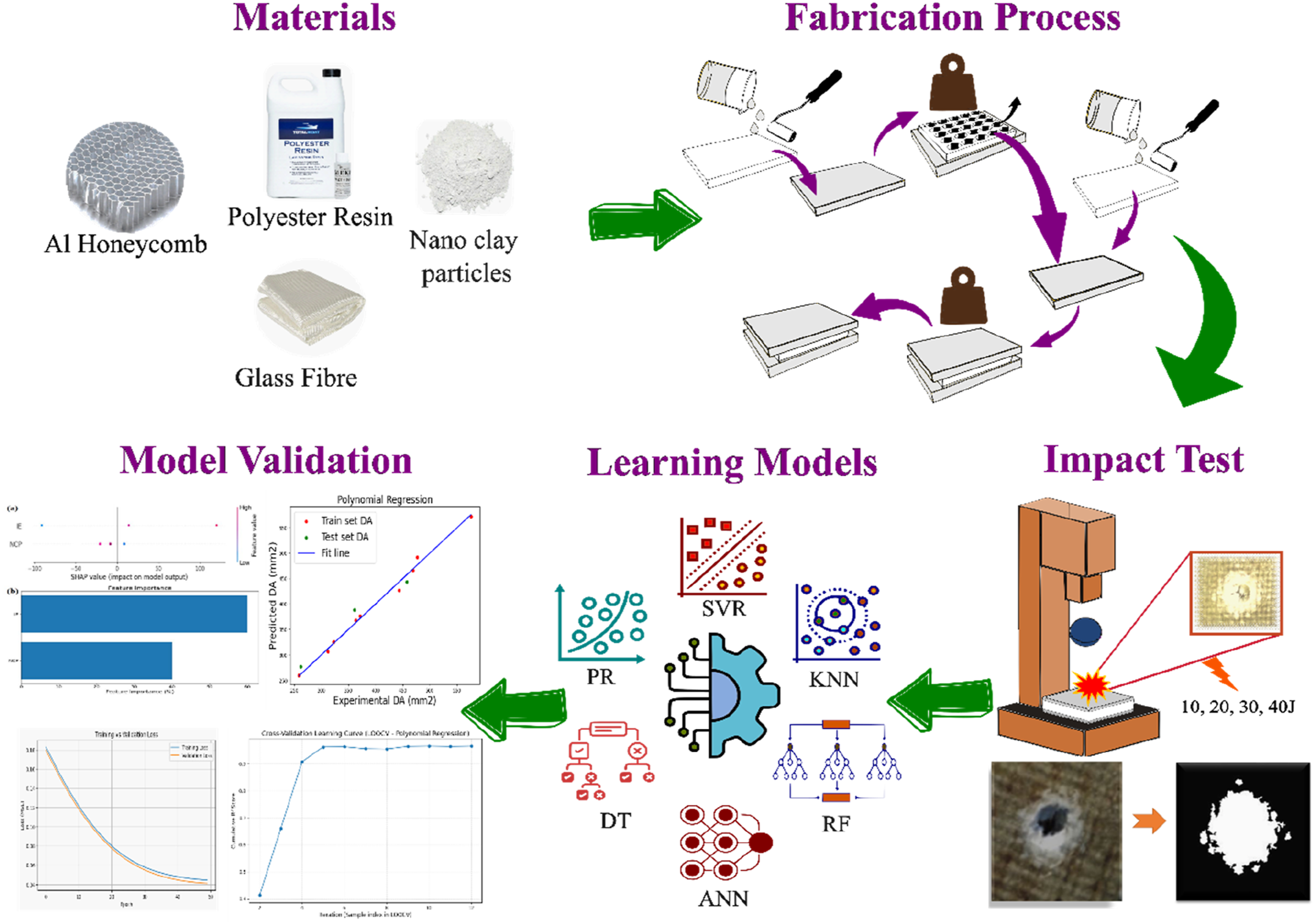
Low-density materials, for example, aluminium honeycomb sandwich panels, are gaining extensive usage in structural applications due to their high strength-to-weight ratio and energy absorption capability. This paper presents the investigations on the low-velocity impact behavior of panels reinforced with nano-clay particles at different contents (0%, 2%, and 4% by weight), fabricated by the hand layup method. Panels were tested under impact energies of 10, 20, 30, and 40 J, and surface damage was quantified using MATLAB image processing to obtain numerical damage area (DA). Five machine learning (ML) models were developed to predict DA, with the Polynomial Regression (PR) model (R² = 0.94) provided a better balance between prediction accuracy and generalization, supported by Cρ (0.90) and LOOCV (R² ≈ 0.95) analyses. SHAP, Feature importance and Partial dependence analysis confirmed impact energy (IE) as the most influential factor, followed by nano-clay percentage (NCP). Experimentally, 2% NCP was identified as the optimal reinforcement level, achieving maximum damage reduction 41% at 10 J, decreasing to 23% at 40 J while 4% NCP yielded marginal additional benefits. Within the 2% NCP, the damage reduction decreased from 41% at 10 J to 23% at 40 J, which further confirms that impact energy is the most dominant factor, as derived from SHAP, feature importance, and Partial dependence analysis. The ANN model presented moderate success regarding the reconstruction of damage features with PSNR values in the range of 13.30–14.81 dB and SSIM scores between 0.62 and 0.64. Overall, integrating experimental analysis with ML modeling offers a robust route to predicting and understanding the impact-induced damage in composite structures.

Graphical Abstract

Keywords

sandwich panel damage area prediction regression model deep learning ANN SHAP

Introduction

Lightweight materials are crucial to all engineering applications where a reduction in structural mass is necessary without sacrificing strength or functionality. The most critical contribution of these materials relates to the improvement of fuel efficiency, enhancement of load-carrying performance, and the provision for more innovative design solutions across different industries, including aviation, vehicle design, and civil engineering.^1–3 The common lightweight materials include aluminum and its alloys, magnesium alloys, titanium, polymer matrix composites, carbon fiber-reinforced plastics, and polymer foams.^4–6 Of these, aluminum honeycomb core sandwich panels are finding greater usage due to their superior strength-to-weight characteristics and excellent capacity for energy absorption..^7,8 This aluminum honeycomb structure, bonded between rigid composite face sheets, has superior stiffness with very low density and enhanced impact resistance compared to conventional monolithic or foam-filled structures. In this configuration, panel thickness can increase to achieve better mechanical performances and energy dissipation without much increase in weight.^9–12 Therefore, aluminum honeycomb core sandwich panels are especially suitable for those applications that require both lightweight construction and high structural efficiency, hence constituting the most relevant material system in designing modern protective and load-carrying components.^13–15

One of the major disadvantages associated with aluminium honeycomb sandwich panels is that they are vulnerable to internal damage when subjected to low-velocity impact loading, resulting in localized failure of the face sheets and core, which compromises structural integrity. The severity of such damage is significantly influenced by the bonding strength at the interface between the core and the face sheets.^16,17 Due to this shortcoming, studies addressing the enhancement of mechanical properties and impact resistance in composite sandwich configurations have been conducted. Recently, researchers have experimentally and numerically analyzed various composite sandwich panels and laminates based on polymers with regard to their mechanical response under conditions of impact loading.

Coupled with experimental efforts, there have been several computational developments to understand plate and laminate impact responses. For instance, the Hp-Cloud meshless approach has been utilized to analyze free vibration in plates with intermediate supports, achieving accurate natural frequency predictions.¹⁸ Similarly, the Spline Finite Strip Method (SFSM) was used to investigate nonlinear low-velocity impacts on tapered laminated composites, highlighting geometric nonlinearity and local indentation effects under eccentric impacts.¹⁹ In early research, improvements in core-to-skin bonding strength and the energy absorption capability of sandwich composites relied on structural modifications such as Z-pinning, stitching, tufting, and polyester pin insertion.^20–26 While these techniques increased interfacial bonding, often they also introduced manufacturing-induced defects into the structures, so matrix modification with nano-fillers became the better method of strengthening the interface without compromising the structural integrity.²⁷

In general, the integration of NCPs into polymer matrices enhances the performance of composite sandwich panels effectively. NCPs enhance matrix stiffness, interfacial adhesion, and load transfer between the core and face sheets, leading to an improvement in delamination resistance, energy absorption, and impact strength. Their high ratio of surface area to volume and the uniform dispersion assures high thermal stability, mechanical strength, and flame resistance. Previous studies have confirmed that reinforcement with NCP increases flexural strength and impact resistance in both glass-fiber composites and AA3003 aluminium honeycomb panels significantly, therefore giving evidence for the potential of nano-scale fillers in enhancing the durability and efficiency of lightweight composite structures.^28–30

Machine learning entering the field of materials and manufacturing had brought a paradigm shift in how researchers analyze complex material behaviors, discover new materials, or optimize manufacturing processes. Traditional experimental methods remain indispensable tools for the impact response and mechanical performance assessment of new materials. However, these are often inextricably linked to extremely time-consuming and labor-intensive procedures involving large volumes of specimen fabrication and testing. On the other hand, ML allows for truly data-driven modeling and prediction of material performance by uncovering correlations between input parameters and the target outcomes, consequently reducing iterative experimentation to accelerate material development and design optimization in a cost-effective manner.^31–34

The capability of ML for the prediction of the mechanical strength, impact response, and energy absorption in the advanced composites has been extensively explored in recent years. XGBoost, RF, GP, and ANN models have emerged as effective models that are capable of providing better forecasting for notched strength and variability in fiber-reinforced polymer laminates. Such models provide enhanced prediction accuracy with reduced generalization error, hence enhancing computational efficiency and structural reliability.³⁵ For example, LR and PR models were used to predict the properties of sandwich panels subjected to low-velocity impacts, and PR coupled with ML algorithms yielded a prediction accuracy of more than 99.9% for maximum energy absorption.³⁶ In another example, ML-based models considering impactor radius, plate thickness, CNT distribution, and impact velocity parameters successfully predicted the low-speed impact response of CNT-reinforced composites. Support vector regression, Gaussian process regression, and linear regression effectively estimated contact force and impact duration, which showed very good agreement with experimental data.³⁷

The potential of deep learning models has also been extended to optimize and design 3D-printed sandwich structures. A recent study, which employed DNNs trained on three-point bending tests, successfully modeled the mechanical behavior of auxetic core beams³⁸. On the other hand, an ICA was used to reduce structural weight with no performance compromise, thus illustrating the combined power of experimental validation, ML, and metaheuristic optimization. These works collectively underline the growing reliance on ML tools with the aim to enhance accuracy, reduce cost, and speed up innovation in material design^39,40. Very recently, works have progressed from numerically driven ML models to image-based approaches, providing deeper insight into material degradation⁴¹. While numerical ML approaches have shown great success in predicting compressive strength, tensile behavior, and energy absorption, they fall short in capturing spatial damage morphology. In contrast, image-based ML and deep learning frameworks identify, classify, and quantify damage zones, thus enriching the understanding of damage geometry and severity.

Notable progress has been made in damage assessment using image-driven techniques. For example, scanning electron microscopy (SEM)-based analyses using support vector machines (SVM), k-nearest neighbors (KNN), and convolutional neural networks (CNN) have demonstrated superior accuracy in distinguishing damaged from undamaged regions, with CNN emerging as the most robust classifier.⁴² Similarly, an ANN-based model trained on modal data effectively localized delamination in sandwich composites with 85% accuracy, though challenges persisted in predicting orientation and extent of damage.⁴³ In another study, unsupervised deep learning methods—specifically convolutional autoencoders (CAE) combined with wavelet-based feature extraction—achieved highly accurate delamination detection in aerospace composites.⁴⁴ Building on these findings, the present study focuses on the image-based prediction of damage area (DA) in NCP-reinforced aluminum honeycomb sandwich panels (NSPs) using deep learning-based ANN models. This approach leverages the strengths of prior ML research while extending it to novel composite configurations and damage prediction through image data analysis.

In the present study, NSPs were fabricated with NCP by the hand layup method with three different weight percentages, i.e., 0%, 2%, and 4%. The impact behavior was studied under low-velocity impact tests at different energy levels ranging from 10 to 40 J. The surface damage was captured using a digital camera. Image processing was done using MATLAB for quality improvement, enhancement of contrast, and making the images uniform to have reproducibility of the results. From the processed images, numerical values of DA were calculated and used to train regression models PR, SVR, KNN, DT, and RF. Similarly, the captured image data was utilized as the input to train deep learning models. ANN architecture was used to predict the area of damage as an image using NCP content and impact energy as inputs. The developed regression models were tested for their precision by R², RMSE, MSE, MAE, and overfitting was checked by the Cρ statistic. Most influencing variables were identified using the SHAP & feature-importance methods. The ANN model developed for image prediction was tested for performance evaluation using training (validation) loss curves, PSNR, and SSIM.

Therefore, the present study establishes a hybrid experimental–computational framework that incorporates low-velocity impact testing with interpretable machine learning modeling to predict and analyze the damage behavior in NCP-reinforced aluminum honeycomb sandwich panels. The novelty in this work includes the following: (i) MATLAB image processing for quantitative damage extraction, (ii) regression and deep learning model implementation for numerical and image-based prediction, and (iii) usage of SHAP and partial dependence analysis to interpret the relative influence of impact energy and nano-clay content. The integrated approach yields new insights into the correlation of reinforcement level, impact energy, and structural damage beyond traditional experimental methodologies.

Materials and methods

Fabrication process

In this study, AA3003 aluminium alloy honeycomb was used as the core material in the fabrication of the sandwich panels. The honeycomb had a hexagonal cell structure with a side length of 6.2 mm, wall thickness of 0.068 mm, core height of 10 mm, and density of 2.7 g/cm³. Reinforcement of the face sheets was made from glass fiber woven fabric with a density of 600 g/m³, laminated in multiple layers. Polyester resin was used for the matrix system, which was then activated with a catalyst of methyl ethyl ketone peroxide and accelerated with cobalt naphthenate. The montmorillonite nano-clay nanofiller used was of more than 99% purity, with 51% SiO₂, 19% Al₂O₃, 0.08% Fe₂O₃ & 3.02% MgO. Nano-clay used was in the form of powder supplied from Ultrananotech Private Limited, Bangalore, having an average particle size of 50–100 nm. It was platelike, layered with an alumino-silicate layer thickness of approximately 1 nm, a density of 1.79 g/cm³, a specific gravity of 2.6, and a pH in the range of 9.5–10.5.

Sandwich panels were manufactured by hand lay-up method at ambient conditions. First, a mold box was prepared and coated with a thin layer of wax as a release agent. Mixing of nano-clay with polyester resin was carried out using a highspeed mechanical stirrer for about 5 min to start the mixing process; this was followed by 1 h of ultrasonic agitation to ensure uniform dispersion of NCP within the resin matrix. After adding the curing agent, the mixture was further mechanically stirred for 2–3 min and left to settle to allow the entrapped air bubbles to come out. This preparation steps are illustrated in the Figure 1.

Figure 1.

Preparation of polyester resin reinforced with nano clay.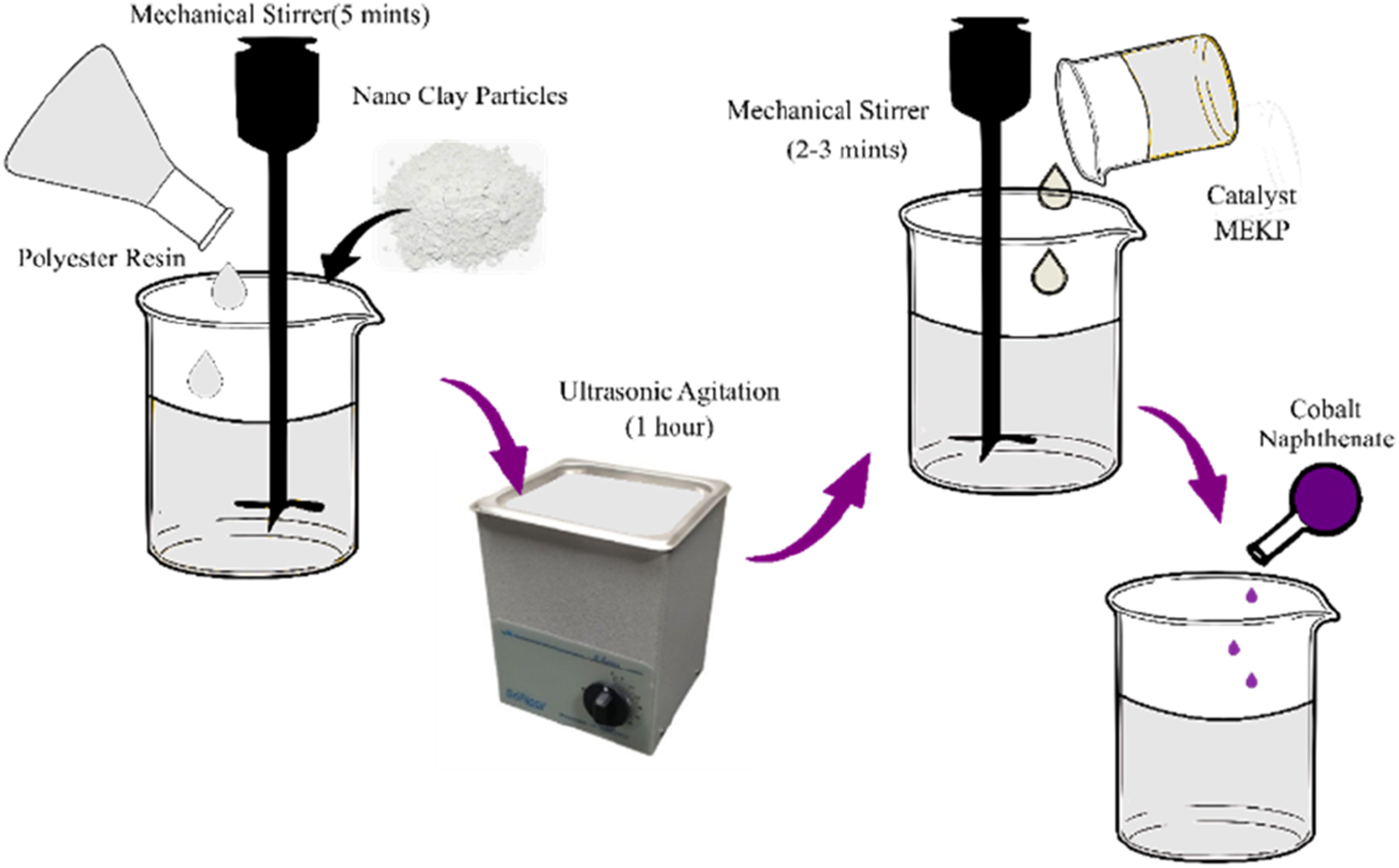

NCP was added to the face sheets at concentrations of 0%, 2%, and 4% by weight to reinforce the structure. The high surface area and multi-layered morphology of the clay enhanced the matrix reinforcement. The nano-clay-infused polyester resin was impregnated into glass fibre woven fabric to form the face sheets. The fabrication of the sandwich panel was completed in two sequential steps. In the initial phase, two layers of glass fibre fabric, pre-impregnated with the NCP–polyester mixture, were affixed to one face of the AA3003 aluminium honeycomb core. This assembly was then subjected to a uniform pressure of 50 kPa and allowed to cure for 24 h. During the second phase, the partially completed panel was turned over, and two more layers of glass fibre fabric were applied to the opposite side, followed by the same curing process. The entire fabrication process fabrication process was carried which is shown in Figure 2. The fabrication process was repeated for each nano-clay concentration. This process resulted in the fabrication of both non-reinforced (SP) and nano-clay-reinforced (NSP) sandwich panels. Specifically, the reinforced panels were designated as NSP2 and NSP4, corresponding to 2 wt.% and 4 wt.% nano-clay, respectively.

Figure 2.

Steps involved in the fabrication of nano clay reinforced sandwich panel.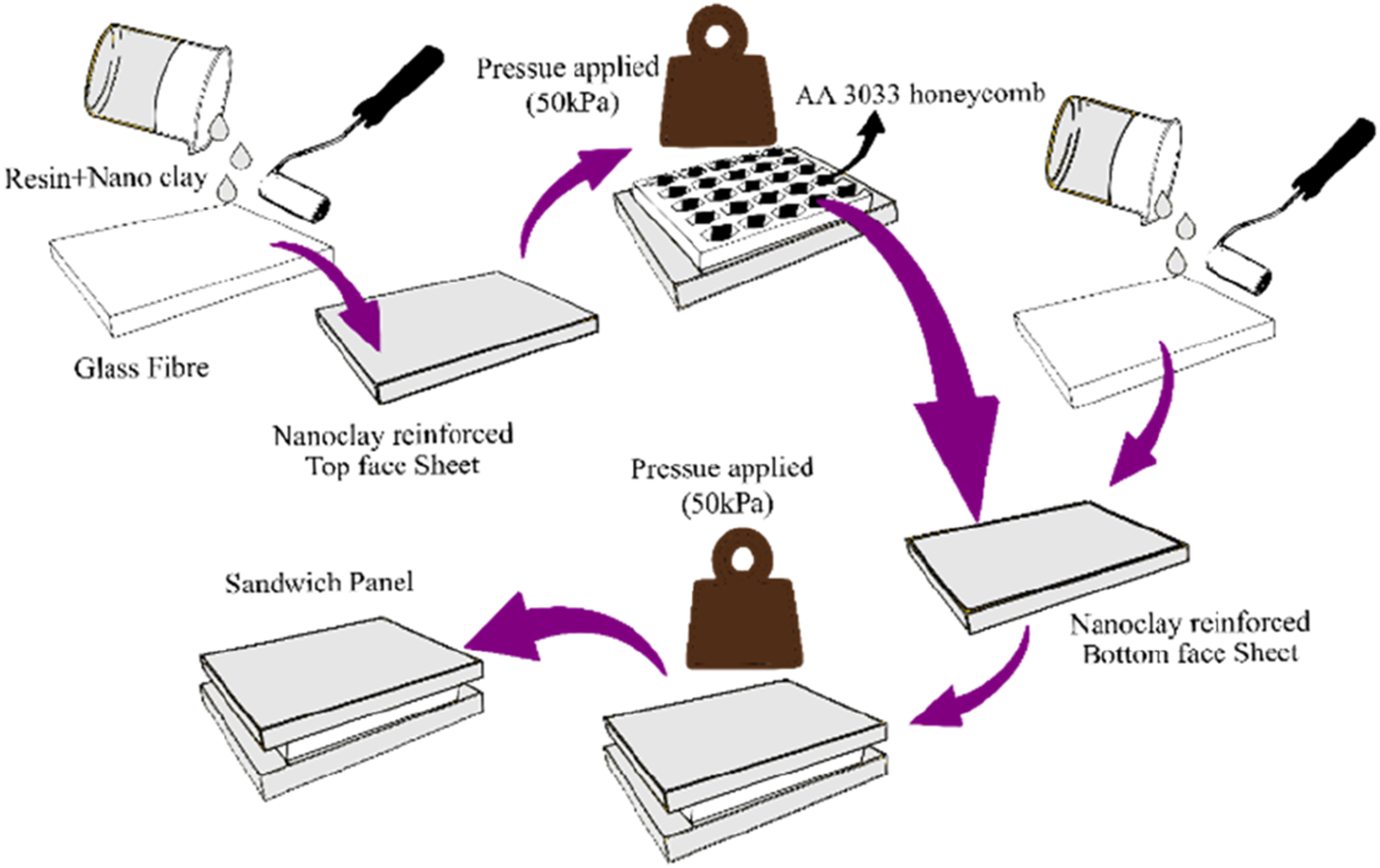

Experimental procedure and test

The Fractovis Plus drop-weight impact machine was utilized to carry out low-speed impact testing in accordance with ASTM D5628-10 specifications. The system included a data acquisition unit that recorded key parameters such as load, velocity, and energy absorbed during impact. Specimens were clamped between circular rings 80 mm in diameter using a pneumatic system for secure placement. A 12.7 mm diameter hemispherical impactor, weighing 4.926 kg, was used in each test and guided along two vertical columns to ensure accurate alignment and impact at the specimen’s center. The impact energies varied between 10 J and 40 J by adjusting the drop height, corresponding to maximum velocities of 4.5 m/s. Figure 3 represents the low-velocity impact test arrangement and sandwich panel measurements.

Figure 3.

(a) Graphical illustration of low velocity impact test, (b) Sandwich panel measurements.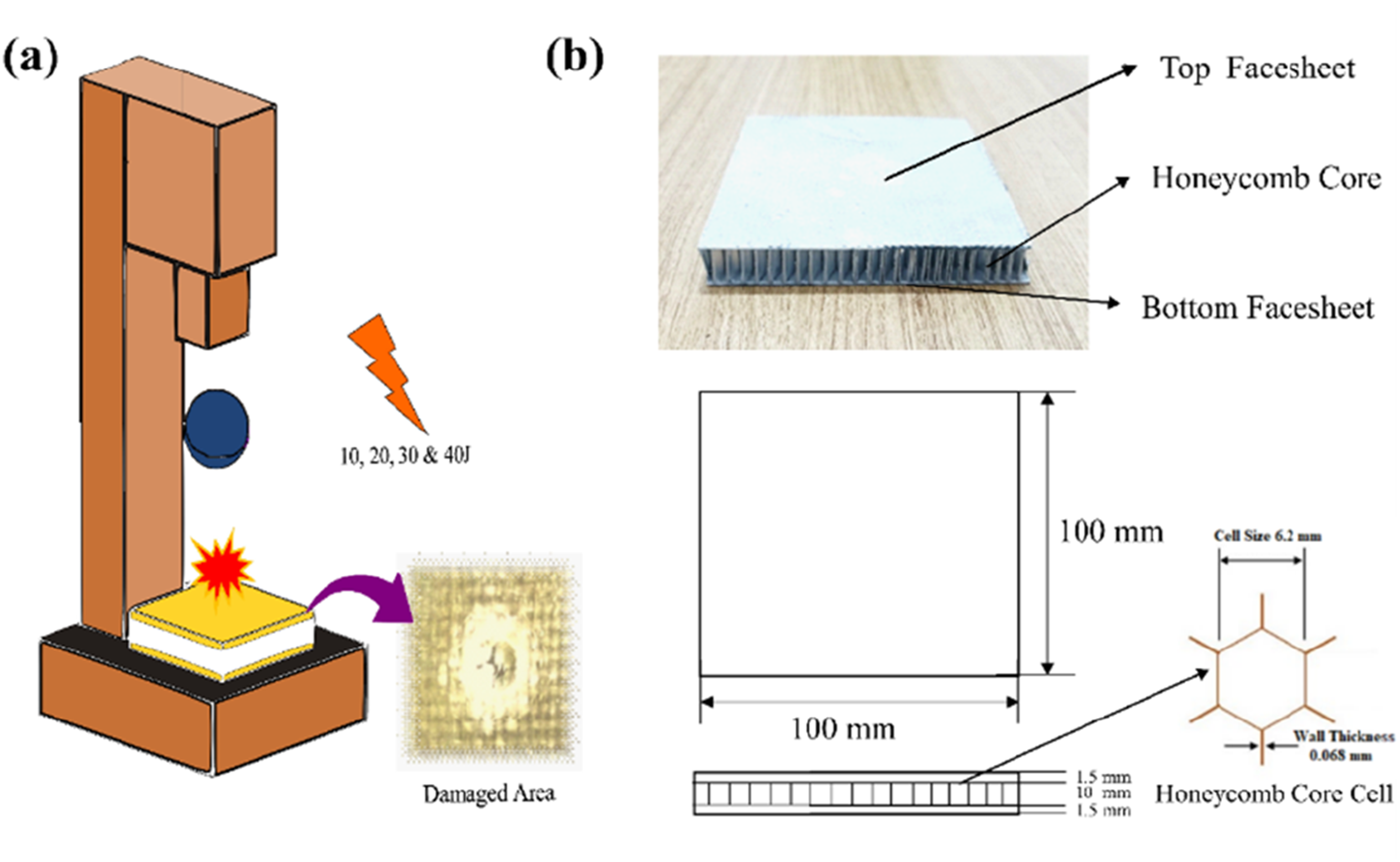

Image processing of damaged area

After impact, the damaged areas of the sandwich panels were recorded with a Nikon D3300 for high-quality pictures. As seen in Figure 4, which shows the arrangement for photographing a damaged specimen, a hollow square frame was placed around the outer region of the damage area to provide a reference area during picture-taking.

Figure 4.

Schematic diagram for image capturing.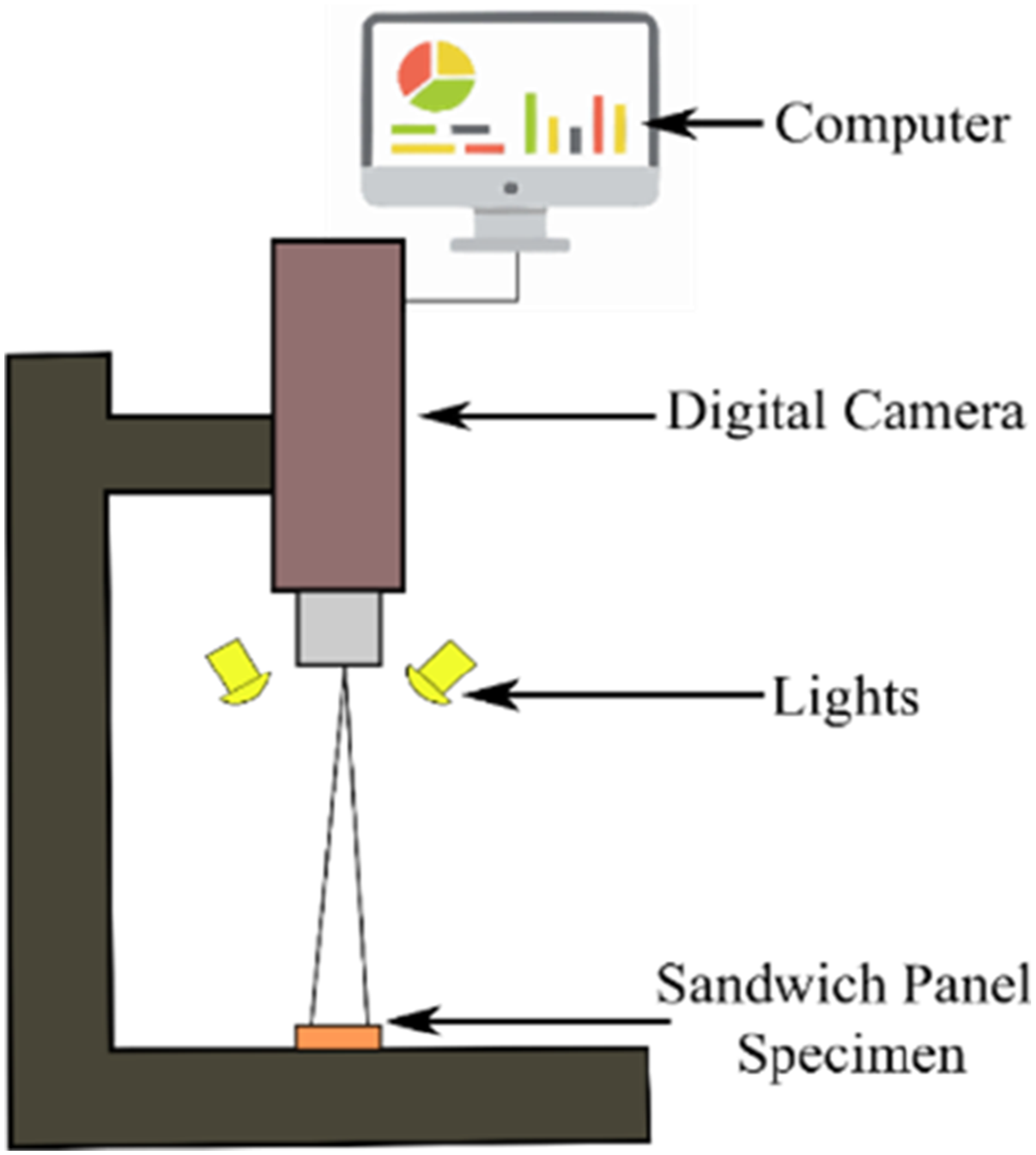

These images were then processed using MATLAB 7.9 to estimate the extent of damage through a systematic image analysis workflow as shown in Figure 5. It started with histogram equalization in order to enhance the image contrast, followed by converting the color image into grayscale and then to a binary image to simplify further analyses. Image segmentation techniques were employed to separate the damaged area from the background.

Figure 5.

Steps involved in the impact damage area processing by MATLAB.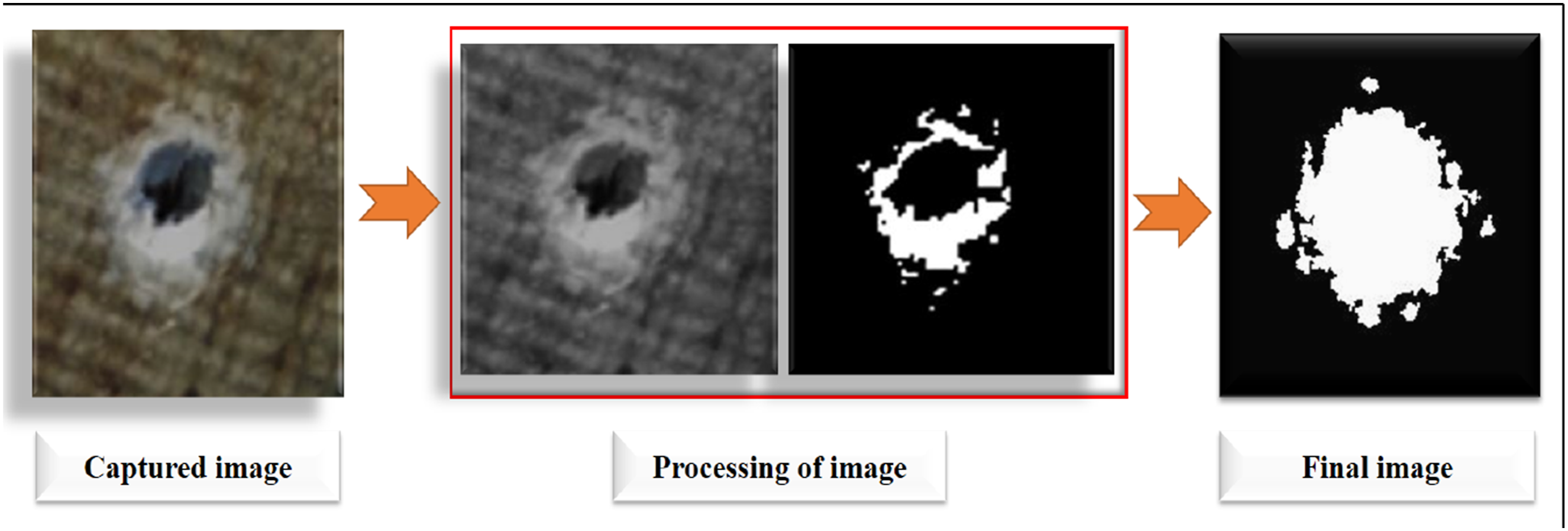

Using MATLAB, the damage extent was computed by deducting the undamaged area from the predefined hollow frame area. Finally, morphological operations such as dilation and erosion were applied to refine the detected region, allowing for accurate identification and measurement of the damage caused by low-velocity impact.

Background of ML

Experimental procedures were initially conducted in this research, followed by MATLAB evaluation of the damage sustained by the specimens. The damage images were processed and converted into structured output formats based on corresponding input parameters. The predictive modeling and training processes were implemented in Python using Google Colab, with the Scikit-learn library utilized for ML operations. Regression models and ANN model were developed to predict the damage area as a numerical value and image output, given specific input variables. These input parameters included the percentage of NCP reinforcement and the applied impact energy. The overall workflow of the predictive modeling and damage evaluation process is illustrated in Figure 6.

Figure 6.

Predictive modelling framework for damage area identification.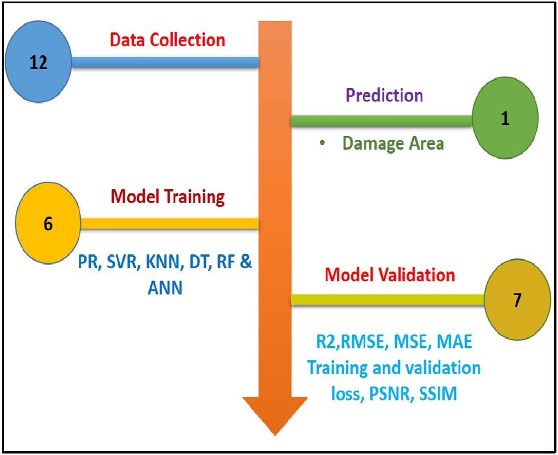

Data collection

The experimental dataset employed for the training and testing the ML-models was derived from the output of image processing performed in MATLAB. The dataset corresponds to varying NCP reinforcement levels (0%, 2%, and 4% by weight) and impact-energy levels ranging from 10 to 40 J. A total of 12 data samples were generated from experimental trials, where the input parameters NCP content and impact energy are represented as numerical data, and the corresponding outputs are image data reflecting the damage area. Figure 7 illustrates the processed output images for the respective input conditions: (a–d) correspond to 0% NCP with impact energies from 10 J to 40 J; (e–h) correspond to 2% NCP with the same range of impact energies; and (i–l) represent 4% NCP reinforcement with impact-energies from 10 to 40 J.

Figure 7.

The output of image processing performed in MATLAB: (a–d) damage area of NSP0; (e–h) damage area of NSP2; and (i–l) damage area of NSP4.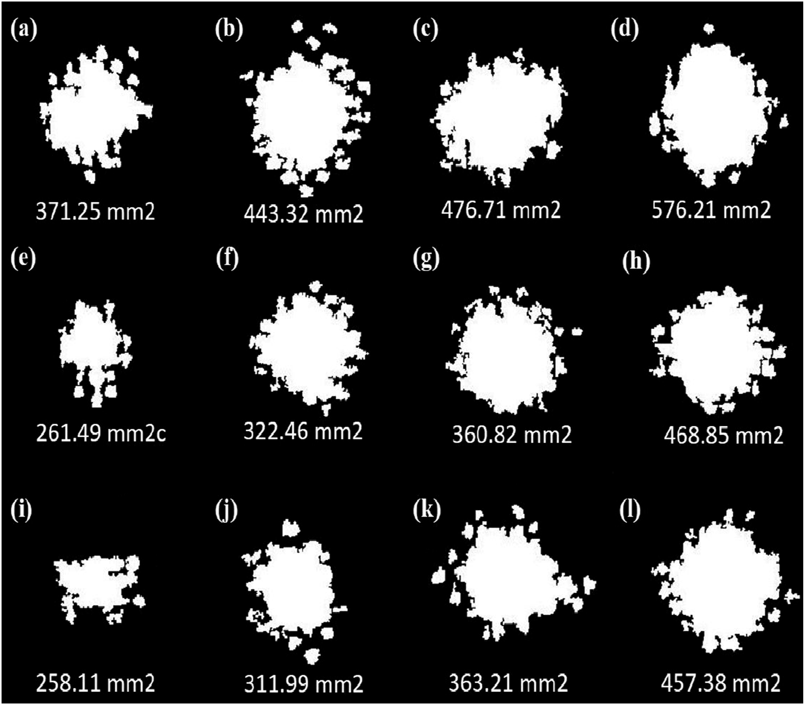

ML models

Regression models

PR is used to model nonlinear interactions between dependent and independent variables by extending linear regression into a quadratic form. This allows for the approximation of curved trends in the data, thereby improving predictive performance when linear models are inadequate. The SVR model with a radial basis function kernel is applied to model complex and nonlinear relations by mapping the input data onto an extended higher-dimension feature space. The performance of SVR is controlled by the hyperparameter settings, including the penalty parameter C, which balances between training error minimization and model generalizability. The KNN algorithm, implemented using K = 2, relies on instance-based learning; namely, a target sample is predicted by referring to the two most similar instances in the feature space, measured by distance metrics. DT generates a tree-like model in a hierarchical manner by recursively splitting the dataset into subsets based on the value of the features. By setting the minimum sample split to 2, DT has the ability to partition data into an arbitrarily small number of subsets, thus better capturing the underlying structure of the data. As an ensemble model, RF integrates outputs from multiple, here 10, decision trees, each developed based on random sampling from the data points and input variables. This ensemble approach further enhances robustness and accuracy in the models while reducing the overfitting risk that might be inherent in individual decision trees.

ANN model

In the present work, an Artificial Neural Network (ANN) was developed as a proof-of-concept model to estimate the damage-area output from the two input variables: NCP reinforcement level and impact energy. The ANN was implemented using the TensorFlow framework and the Keras API. Based on the limited number of available experimental samples (n = 12), a simplified sequential architecture was adopted to reduce the risk of overfitting. The final ANN architecture consisted of a single hidden layer with 10 neurons, using the ReLU activation function. ReLU was selected because it provides fast convergence and avoids vanishing-gradient issues when mapping nonlinear relationships in small datasets. The output layer contained a number of neurons equal to the 50 principal components retained from PCA, which reduced each 244 × 244 damage image to a lower-dimensional representation preserving 98% of the variance. A linear activation function was used in the output layer because PCA components are continuous real-valued quantities that may take both positive and negative values. The model was trained using the Mean Squared Error (MSE) loss function and the Adam optimizer, which adaptively tunes the learning rate and performs efficiently on sparse gradient problems. Training was conducted for 50 epochs with a batch size of 8. The dataset of 12 samples was split into an 80/20 ratio, resulting in nine training samples and three validation samples, ensuring consistent and reproducible evaluation of the model’s generalization ability despite the small sample size. This ANN configuration allowed the model to learn an approximate mapping between the numerical input parameters and the PCA-compressed damage-area representations. Because of the limited dataset, this ANN-based prediction is presented strictly as a proof-of-concept, demonstrating feasibility rather than serving as a robust deep-learning predictive framework. The architecture of the developed ANN is shown in Figure 8.

Figure 8.

ANN topology used for ANN predictive modelling.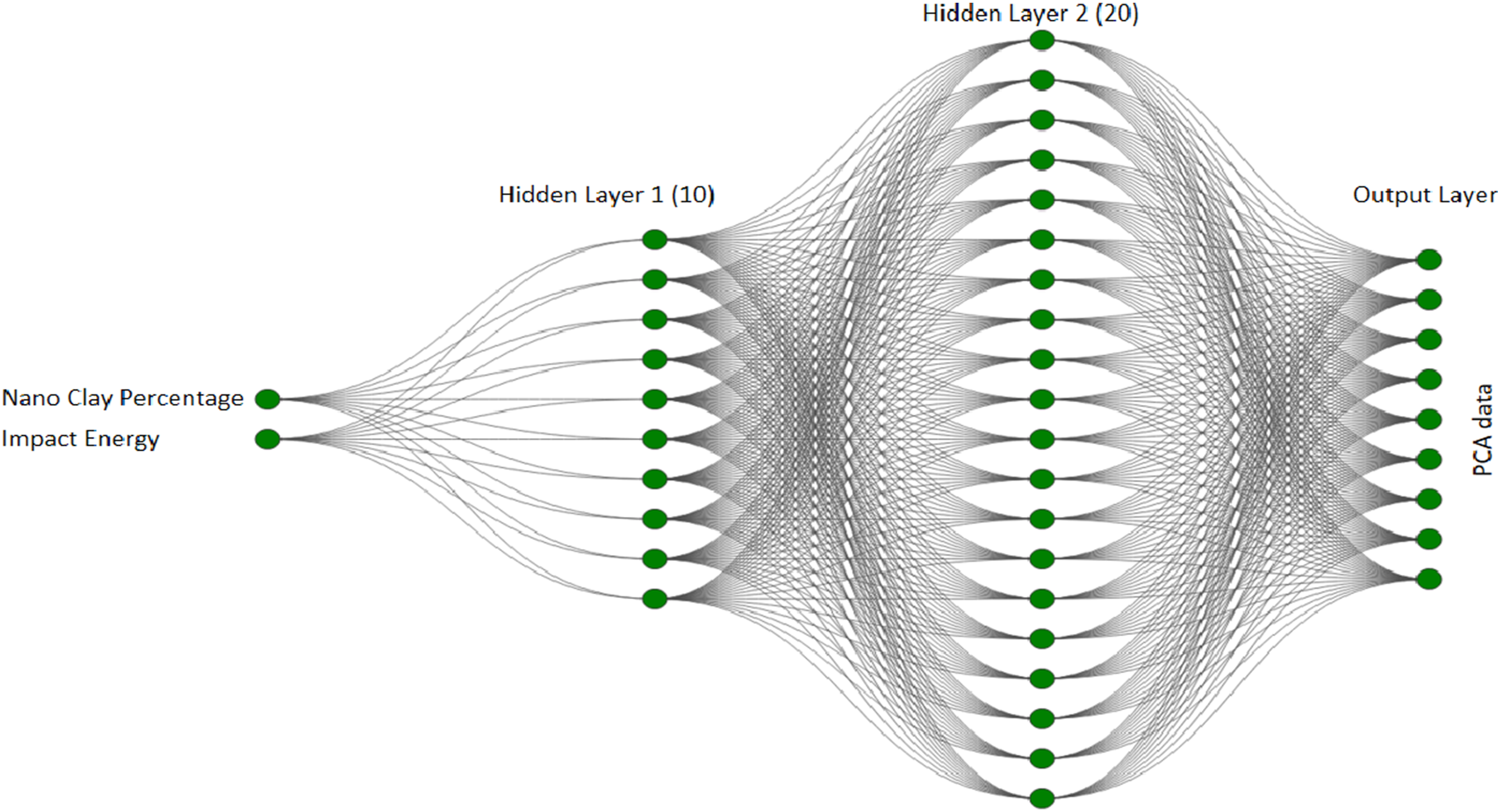

Model validation

Model validation for regression models

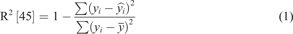
Model validation refers to the assessment of a trained model’s ability to accurately predict outcomes for given inputs. It ensures the reliability and generalization capability of the model by evaluating its performance on unseen data. A common and critical approach to validation involves splitting the dataset into 80% for training and 20% for testing, where the training set is used to build the model and the testing set is used to assess its predictive accuracy. Some of the metrics to judge model performance include R², RMSE, MSE, MAE, and Cρ. The R² is a value between 0 and 1. 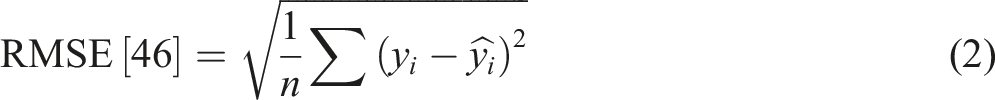A value close to 1 denotes a good performance and excellent accuracy in predicting.⁴⁵ On the other hand, if this value is close to 0, then the model is poor in predicting the output. In the case of RMSE, MSE, and MAE, the best model has the lowest values because these represent the average of the errors in predictions. 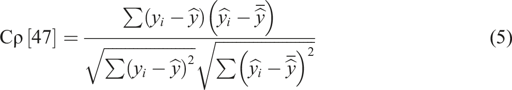The smaller the error value, the closer the predicted output-values to the actual values.⁴⁶ The Cρ measures the actual and expected values regarding linear correlation. A high value of Cρ close to 1 indicates a high correlation and, hence, a successful model. This coefficient will be independently computed for both the training and test sets.⁴⁷ If the Cρ from the test set is higher than the Cρ from the train set, then the model is also doing a good job on the unseen data with no overfitting. If Cρ from the test set is substantially lower compared to the Cρ from the train set, then there is overfitting possibly because of noisy data.

R^{2} [45] = 1 - \frac{\sum {(y_{i} - \hat{y_{i}})}^{2}}{\sum {(y_{i} - \bar{y})}^{2}}

(1)

where:

• $y_{i}$ = True values

• $\hat{y_{i}}$ = Anticipated values

• $\bar{y}$ = Mean of true values

RMSE [46] = \sqrt{\frac{1}{n} \sum {(y_{i} - \hat{y_{i}})}^{2}}

(2)

MSE [46] = \frac{1}{n} \sum {(y_{i} - \hat{y_{i}})}^{2}

(3)

MAE [46] = \frac{1}{n} \sum | y_{i} - \hat{y_{i}} |

(4)

C ρ [47] = \frac{\sum (y_{i} - \hat{y}) (\hat{y_{i}} - \bar{\hat{y}})}{\sqrt{\sum {(y_{i} - \hat{y})}^{2}} \sqrt{\sum {(\hat{y_{i}} - \bar{\hat{y}})}^{2}}}

(5)

Model validation for ANN

The performance of a ML-model is generally monitored by looking at its training and validation loss. Training loss tells how well the model fits the training dataset, while the validation loss estimates its performance on unseen inputs. Both are computed at the end of every epoch on training and validation datasets, respectively. A low training and validation loss indicates good learning, whereas an increasing validation loss may point towards overfitting of the model.⁴⁸ Effective validation involves monitoring losses, tuning hyperparameters, and applying techniques like early stopping.

MSE (Loss) [49] = \frac{1}{n} \sum {(y_{i} - \hat{y_{i}})}^{2}

(6)

where:

• $y_{i}$ = True values

• $\hat{y_{i}}$ = Anticipated values

PSNR actually quantifies the fidelity of a reconstructed image from the original one, using MSE as the basis. It is expressed in decibels, and the higher the PSNR, the better the quality of the image with less noise or degradation^49,50. To validate using PSNR, MSE is computed between the original and output images, then apply the PSNR formula:

PSNR [49] = 10 . \log_{10} (\frac{M A X^{2}}{M S E})

(7)

where:

• MAX is the maximum possible pixel value

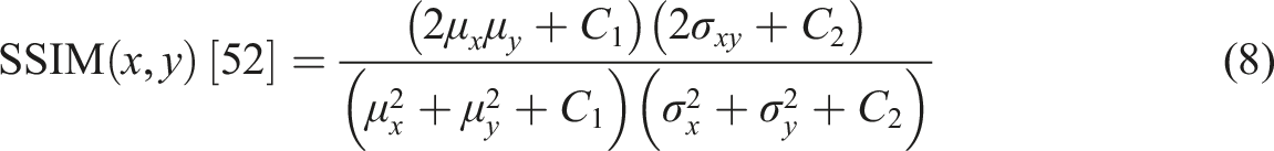
Traditional error metrics comprise SSIM on image similarity, given that such a measure considers factors related to perceived visual quality, such as structure, light intensity, and contrast. Unlike PSNR or MSE, SSIM is much more in line with human visual perception. It outputs a value between −1 and 1, where 1 means perfect similarity. A higher SSIM (>0.9) indicates high-quality preservation of image content and structure.^51,52

SSIM (x, y) [52] = \frac{(2 μ_{x} μ_{y} + C_{1}) (2 σ_{x y} + C_{2})}{(μ_{x}^{2} + μ_{y}^{2} + C_{1}) (σ_{x}^{2} + σ_{y}^{2} + C_{2})}

(8)

where:

• $x, y$ two image patches

• $μ_{x} μ_{y}$ mean (average intensity) of images $x$ and $y$

• $σ_{x}^{2}, σ_{y}^{2}$ variance of $x$ and $y$

• $σ_{x y}$ covariance between $x$ and $y$

• $C_{1}, C_{2}$ small constants to stabilize the division

• $C_{1} = {(K_{1} . L)}^{2}$

• $C_{2} = {(K_{2} . L)}^{2}$

• L is the dynamic range of pixel values, and $K_{1}$ = 0.01, $K_{2}$ = 0.03

Leave-one-out cross-validation (LOOCV)

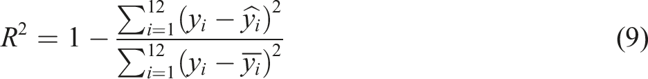
LOOCV is a resampling technique in which a dataset containing n samples is used n times to train the model, where in each iteration one sample is left out for testing and the remaining n−1 samples are used for training, ensuring that every sample is used exactly once for validation. The model performance is estimated by aggregating the evaluation results from all n runs, typically by averaging an error metric or, in regression problems, by computing a cumulative coefficient of determination. LOOCV is an extreme case of k-fold cross-validation with k = n, which maximizes training data usage and is particularly suitable for small datasets. Although it provides a low-bias estimate of model performance, it often exhibits higher variance due to single-sample testing and is computationally expensive because the model must be retrained multiple times; however, for certain models such as linear regression, efficient analytical solutions exist to compute LOOCV errors without repeated retraining. After generating predictions for all left-out samples, the model is validated using the cumulative R², the cumulative R² was calculated as follows:

R^{2} = 1 - \frac{\sum_{i = 1}^{12} {(y_{i} - \hat{y_{i}})}^{2}}{\sum_{i = 1}^{12} {(y_{i} - \bar{y_{i}})}^{2}}

(9)

where

y_{i}

is the actual value,

\hat{y_{i}}

is the predicted value from LOOCV for sample iii, and

\bar{y_{i}}

is the mean of all actual values, with higher cumulative R² indicating better predictive performance and generalization, as illustrated by the systematic LOOCV workflow in Figure (9).

Figure 9.

Systematic process of cross validation (LOOCV).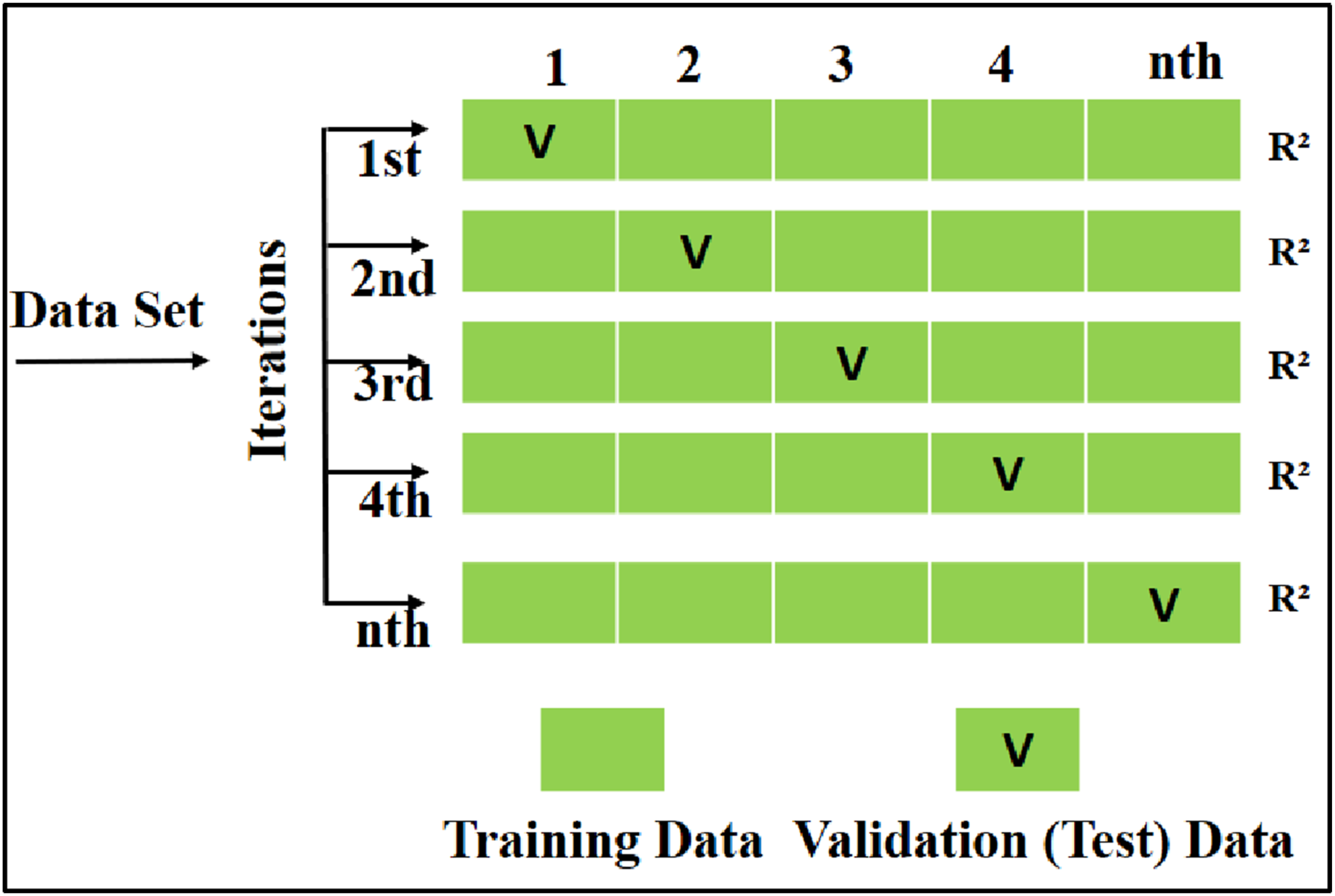

Result and discussion

Regression model assessment on DA prediction

Figure 10(a)–(e) presents a comparative assessment of the predicted and experimentally measured DA values through five different regression models. In each subplot, the blue diagonal line represents the ideal case of perfect prediction where predictions perfectly match actual experimental findings. Red and green markers denote the training and test data, respectively, which can be considered as indications of the fitting and generalization performance of models. Among all models, DT and PR achieves the best predictive accuracy with most points other than one located close to the reference line. This means that the DT and PR model performs much better in predicting DA values with high accuracy. In contrast, SVR, KNN, and RF models present higher dispersion of the points away from the reference line. Such deviation reflects that these models demonstrate relatively low predictive precision and hence may underperform compared with DT and PR in this application.

Figure 10.

Experimental DA from dataset versus predicted DA by (a) PR, (b) SVR, (c) KNN, (d) DT and (e) RF.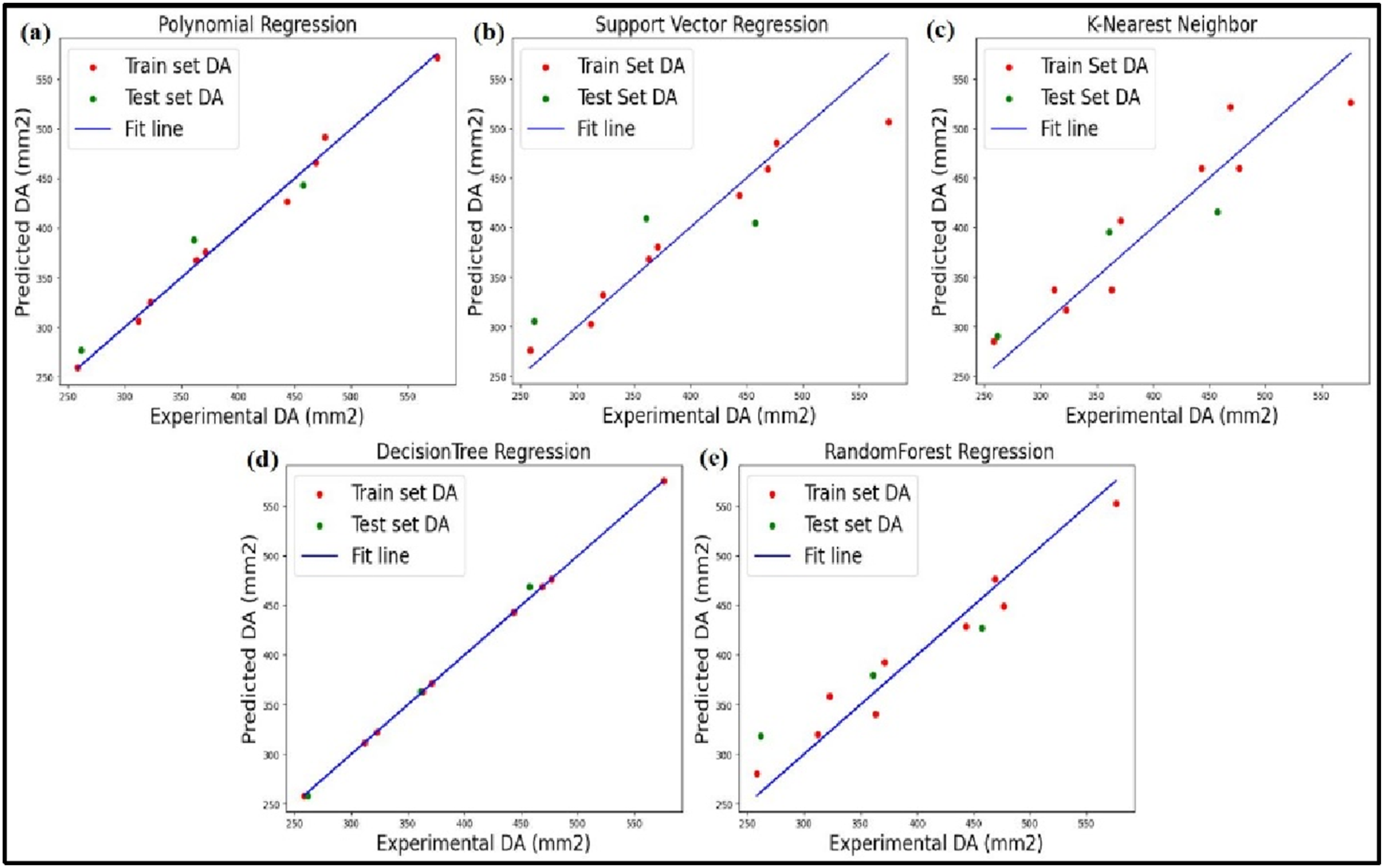

To comprehensively assess the predictive performance of the ML models in forecasting DA values, several statistical performance metrics were employed. These included the coefficient of determination (R²), Mean Absolute Error (MAE), Mean Squared Error (MSE), and Root Mean Squared Error (RMSE). These metrics are represented in Figure 11(a)–(d). Among the five models, the DT and PR showed the highest overall performance, with the highest R² value of 0.99 and 0.93 and the lowest MAE, MSE, and RMSE values, respectively. The high R² value agrees with the visual performance analysis of the DT and PR model in Figure 10(d), where all data except one outlier lie very close to the ideal reference line. This depicts excellent model fit with high prediction accuracy. By contrast, SVR, KNN, and RF models achieved lower R² values of 0.63, 0.80, and 0.76, respectively. The comparative low scores obtained for these metrics reflect poor predictive reliability and higher deviation from the actual DA values. These results evidently indicate that the PR and DT models present the best performance for all other models in predicting DA of NSPs. Strong statistical indicators and near-perfect alignment with experimental data justify its suitability for being the best regression model in this work.

Figure 11.

Quantitative evaluation of the five ML models on DA. (a) R², (b) RMSE, (c) MSE and (d) MAE.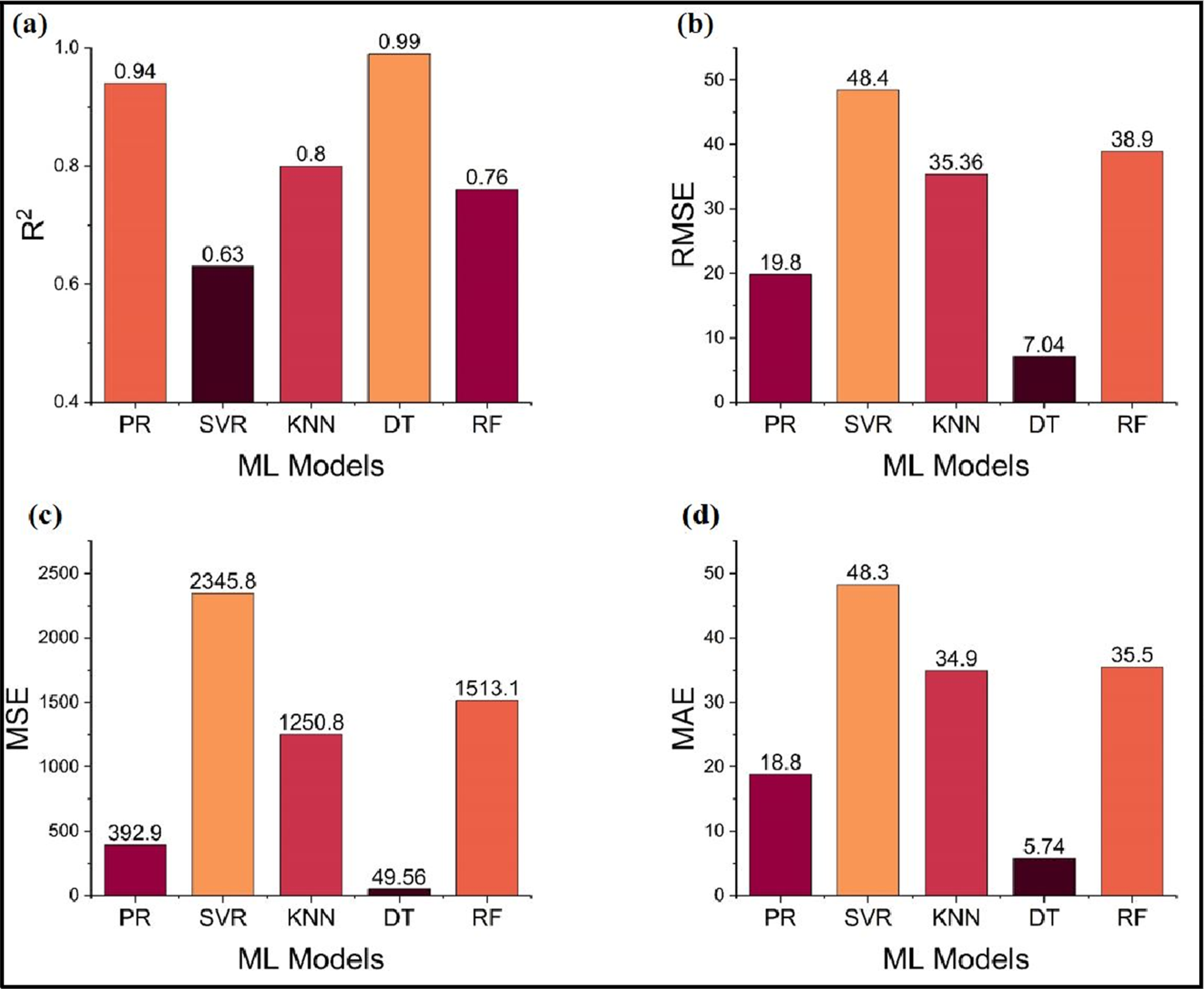

Assessment on overfitting

Figure 12(a) shows that the residual plot for the PR model with degree 2 has relatively small and centered residuals for the training set, while for the test set, residuals are more dispersed and noticeably deviate from the zero line. This means that this model fits better for the training data than for the unseen test data, which implies mild overfitting. While the quadratic model captures the general trend of the data, the bigger spread of residuals in the test set is indicative of a limited generalization capability. The PR model performs decently with slight overfitting, possibly due to fewer data points, which can be further optimized by using regularization or cross-validation-based optimization.

Figure 12.

Residual plots for the prediction of DA (a) PR, (b) DT.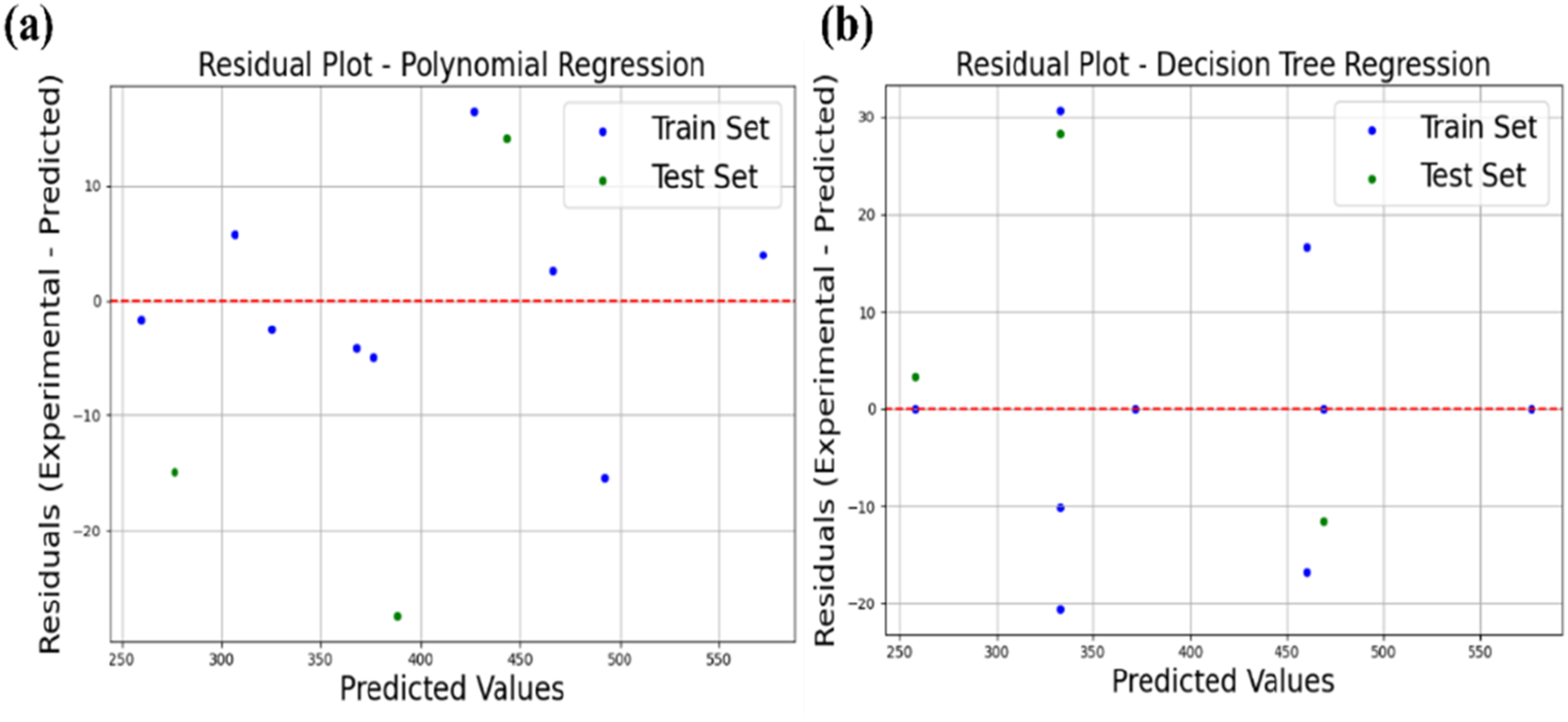

Figure 12(b) shows that the residual plot of the DT Regression model has several training points with zero residuals, indicating perfect predictions and a stronger tendency toward overfitting. In contrast, the test residuals display larger deviations and inconsistent distribution around the zero line, revealing weaker generalization to unseen data. Although the DT model achieved a higher R² value (0.99) compared to the PR model (R² = 0.94), the residual analysis confirms that the DT model suffers from more pronounced overfitting. The PR model, on the other hand, exhibits only slight overfitting and provides a more balanced trade-off between training accuracy and generalization performance.

Pearson correlation of the PR model

The Pearson correlation coefficient, Cρ (−1 to +1), quantifies the strength and direction of the linear relationship between predicted and actual values. A Cρ value close to +1 implies a strong positive linear correlation; that is, predictions increase proportionally with actual observations. This would therefore mean that the model has high predictive consistency. Conversely, a Cρ close to −1 indicates a strong negative/inverse relation, while a value close to 0 indicates little or no linear relationship, which means poor alignment between predicted and actual outputs. Though Cρ does not directly diagnose model accuracy in terms of variance explanation, as would be done by the coefficient of determination, R²,⁵³ it is useful in the diagnosis of overfitting tendencies. Overfitting is usually characterized by a high value of Cρ for the training data but substantially lower values for the test data, evidence that the model may be memorizing rather than learning generalizable features in the training data.^54,55

Figure 13 compares the Cρ values of the PR model on predicting DA in both the training and test datasets. In the training set, the Cρ value is 0.96, while in the test set, this slightly decreases to 0.90. This slight decrease in values means there is mild overfitting, likely because of the small size of the dataset. On the whole, this model performs acceptably, with only slight overfitting that could easily be improved by regularization techniques or cross-validation-based optimization.

Figure 13.

Comparison of pearson correlation (Cρ) for training and test sets across PR model on predicting DA.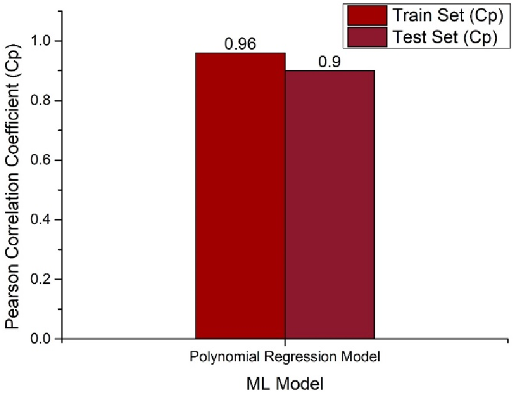

Assessment on LOOCV

Figure 14 illustrates the LOOCV learning curve for the degree-2 PR model using a small dataset of 12 samples, where each sample is successively left out for testing while the remaining samples are used for training. After all iterations, the cumulative R² is computed using the complete set of LOOCV predictions, providing an overall measure of predictive performance rather than an average of individual iteration scores. The curve indicates that the initial R² value is relatively low (around 0.4), reflecting high variability when only a few iterations are considered; however, as more iterations are incorporated, the R² increases rapidly and stabilizes near 0.95, demonstrating strong predictive capability. The minor fluctuations observed in the intermediate region highlight the sensitivity of the model to individual data points, which is characteristic of LOOCV applied to small datasets, but the overall upward and stable trend confirms that the degree-2 PR model generalizes well despite the limited sample size.

Figure 14.

LOOCV learning curve of the PR model for DA prediction.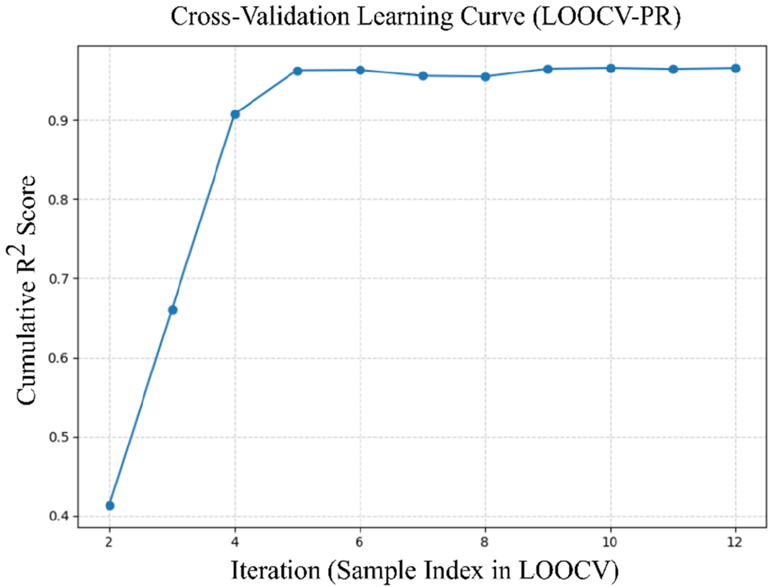

Model interpretation

SHAP (SHapley Additive exPlanations) is a powerful tool used to interpret the influence of input parameters on the output prediction of ML models. In a SHAP summary plot, each dot corresponds to a single prediction, with the color indicating the actual value of the feature (red for high, blue for low, and purple for medium). The features are arranged from top to bottom in order of decreasing importance, and a wider spread of SHAP values signifies a greater impact on the model’s prediction. Positive SHAP values indicate that a feature increases the predicted output, while negative values suggest a decreasing effect.^56,57

The interpretability analysis presented in Figure 15 is based on the PR model, which was selected as the final regression model for predicting the DA. These analyses were conducted specifically on the PR model to quantify the relative influence of IE and NCP on the model output. Figure 15(a) shows the SHAP summary plot, where IE exhibits a substantially wider range of SHAP values than NCP. This indicates that variations in IE induce stronger positive and negative shifts in the predicted DA, thereby demonstrating its dominant influence within the model. In contrast, the narrower spread of SHAP values for NCP reflects a comparatively weaker but still meaningful impact on the prediction. The SHAP feature importance plot in Figure 15(b) reinforces this interpretation: the PR model assigns a higher relative importance to IE, whereas NCP contributes to a lesser extent. It is important to emphasize that the reported ratios (60% for IE and 40% for NCP) represent model-derived relative importance metrics and should not be interpreted as physical contribution percentages due to the limited dataset and the presence of only two input variables. The PDP results in Figure 15(c) further elucidate the variable response relationships. As NCP increases from 0 to 4 wt%, the DA exhibits only a moderate decreasing trend, suggesting that higher nano clay content marginally enhances interfacial bonding and stiffness, thereby improving the composite’s ability to dissipate impact energy. Conversely, DA increases pronouncedly with an increase in IE from 10 J to 40 J, indicating that the composite’s damage response is highly sensitive to impact load. Higher IE levels induce greater deformation and crack propagation, resulting in significantly larger damage areas. The interpretability is further supported by the PR model equation, which is expressed as follows and explicitly quantifies the influence of each input variable on DA.

DA = 340.2517 - 69.5721 NCP + 2.8606 IE + 10.3719 {NCP}^{2} - 0.1039 (NCP \times IE) + 0.0735 {IE}^{2}

(10)

Figure 15.

Model interpretation on DA prediction (a) SHAP, (b) Feature importance, (c) Partial dependence.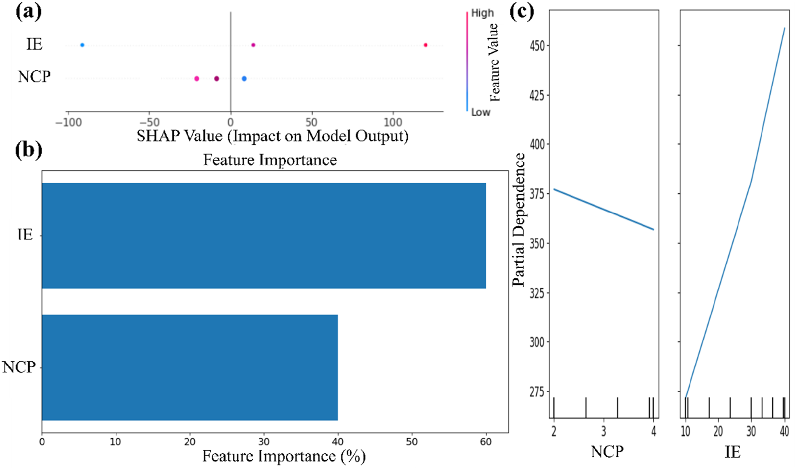

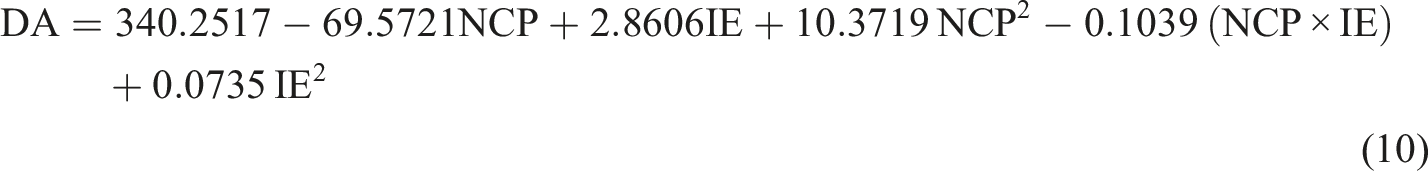
The negative linear coefficient of NCP and its positive quadratic term indicate a mild, nonlinear moderating effect on damage, whereas the strong positive linear and quadratic coefficients of IE confirm that impact energy is the dominant factor driving increases in DA, consistent with the SHAP, Feature importance and PDP analyses.

Influence of nano-clay and impact energy on damage area

The addition of NCP significantly affected the damage behavior of aluminium honeycomb sandwich panels under low-velocity impact. At all the impacting energies considered, NSPs exhibited a much smaller damaged area in comparison with the unreinforced panels, NSP0, showing enhanced resistance to impact and energy dissipation capabilities.

Figure 16 (a)–(d) show the correlation of nano-clay percentage, 0%, 2%, and 4%, with damage area for constant impact energies of 10 J, 20 J, 30 J, and 40 J, correspondingly. In the case of 10 J impact energy, Figure 13(a) indicates a significant 41% reduction of the damage area upon increasing the NCP content from 0% to 2% (NSP0–NSP2). Further increasing the NCP to 4% results in limited further improvement (NSP4). Similar trends occurred for higher impact energies; the respective reductions of damage area from NSP0 to NSP2 were 37%, 32%, and 23% for 20 J, 30 J, and 40 J, respectively. These results indicated that nano-clay reinforcement improves impact resistance considerably but with diminishing return as the impact energy increases. These improvements could be attributed to the intrinsic properties of nano-clay particles, such as their high-aspect-ratio geometry, large surface area, and strong interfacial adhesion with the polymer matrix. Such properties allow the NCP to operate at the nanoscale level as reinforcements, delaying or diffracting the crack, improving the matrix-to-fiber stress transfer, and acting as a barrier for localized energy concentration. This results in more homogeneous load transfer with less extensive impact-induced damages. Furthermore, it was observed that for a constant reinforcement level, the efficiency of NSP2 in mitigating damages decreases by increasing impact energy from 41% at 10 J to 23% at 40 J. This implies that while structural resilience is enhanced using nano-clay reinforcement, impact energy remains as one of the predominant factors controlling damage severity. The above experimental observations are in good agreement with the SHAP analysis and importance scores from the developed predictive model, which confirmed that model performance and experimental observation appeared with strong positive correlations.

Figure 16.

DA versus NCP (0%, 2%, 4%) for panels impacted at (a) 10 J, (b) 20 J, (c) 30 J, and (d) 40 J.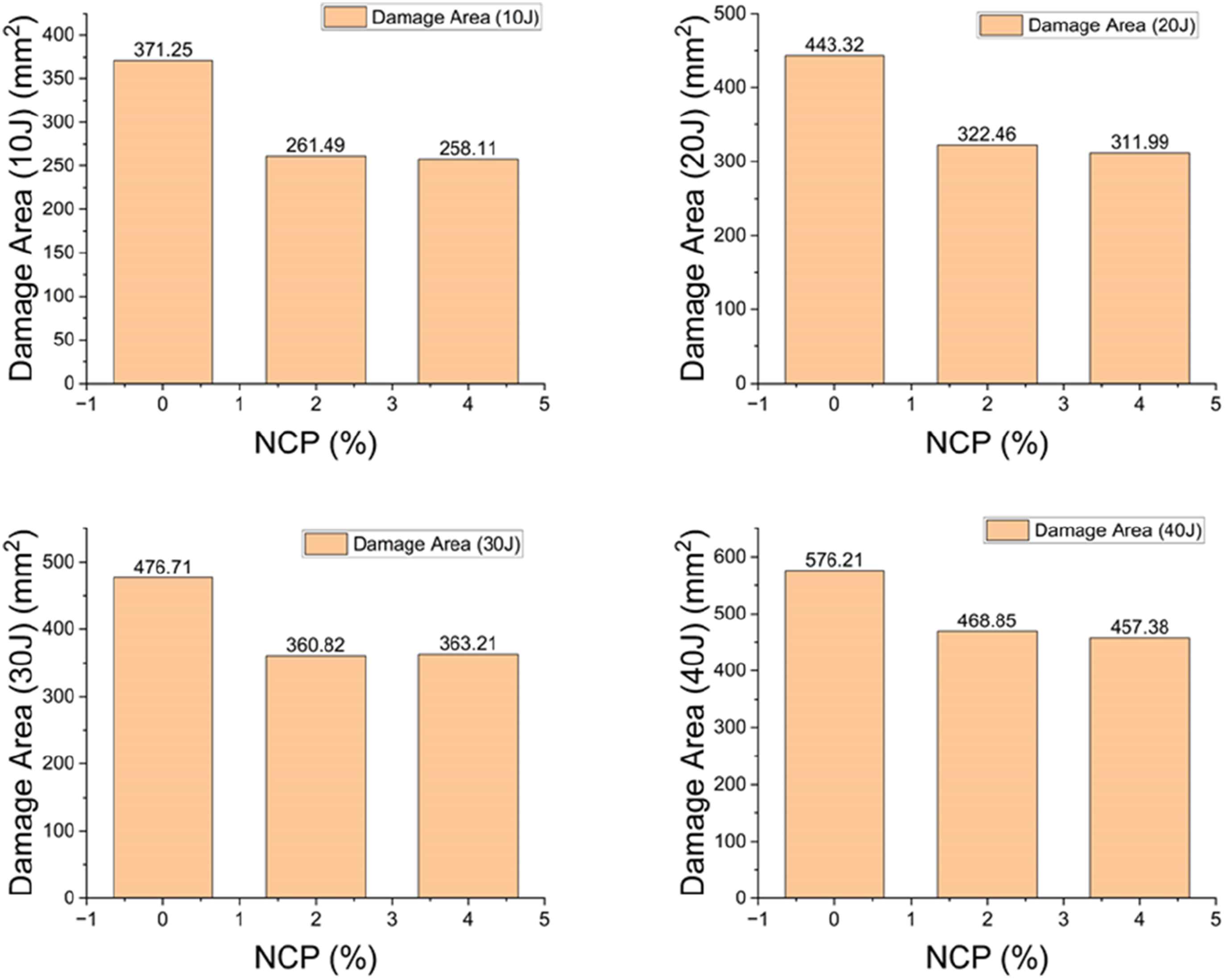

ANN model assessment on prediction of damage area

Figure 17 depicts the training and validation loss curves for the ANN model during 50 epochs. The x-axis is used to plot the number of epochs, ranging from 0 to 50, each representing an iteration of learning by the model from the data. The y-axis is the value for loss, calculated using MSE, reflecting the difference between the predicted and actual value. The blue curve represents the training data set, while the orange one indicates the validation data set. It can be observed that with an increase in the number of epochs, the loss in training keeps decreasing, which means the model learns well the underlying patterns of the training data. Similarly, the loss in validation decreases with an increase in the number of epochs, which indicates that the model generalizes well for unseen data and predicts values quite accurately. The curves show a similar trend of going downwards without significant divergence, which means that the performance of the model is consistent for both training and validation data. As can be seen, the validation loss is less than the training loss during the entire training process. This signifies that this model does not overfit and gives better performance on unseen data. The MSE value at the 50th epoch reaches 0.0479 for validation loss, which is close to zero. A lesser value of MSE signifies that the model is highly accurate in prediction. Thus, it proves the effectiveness of the model in predicting the damage area of the images with a very low error.

Figure 17.

Training and validation comparison for the ANN model.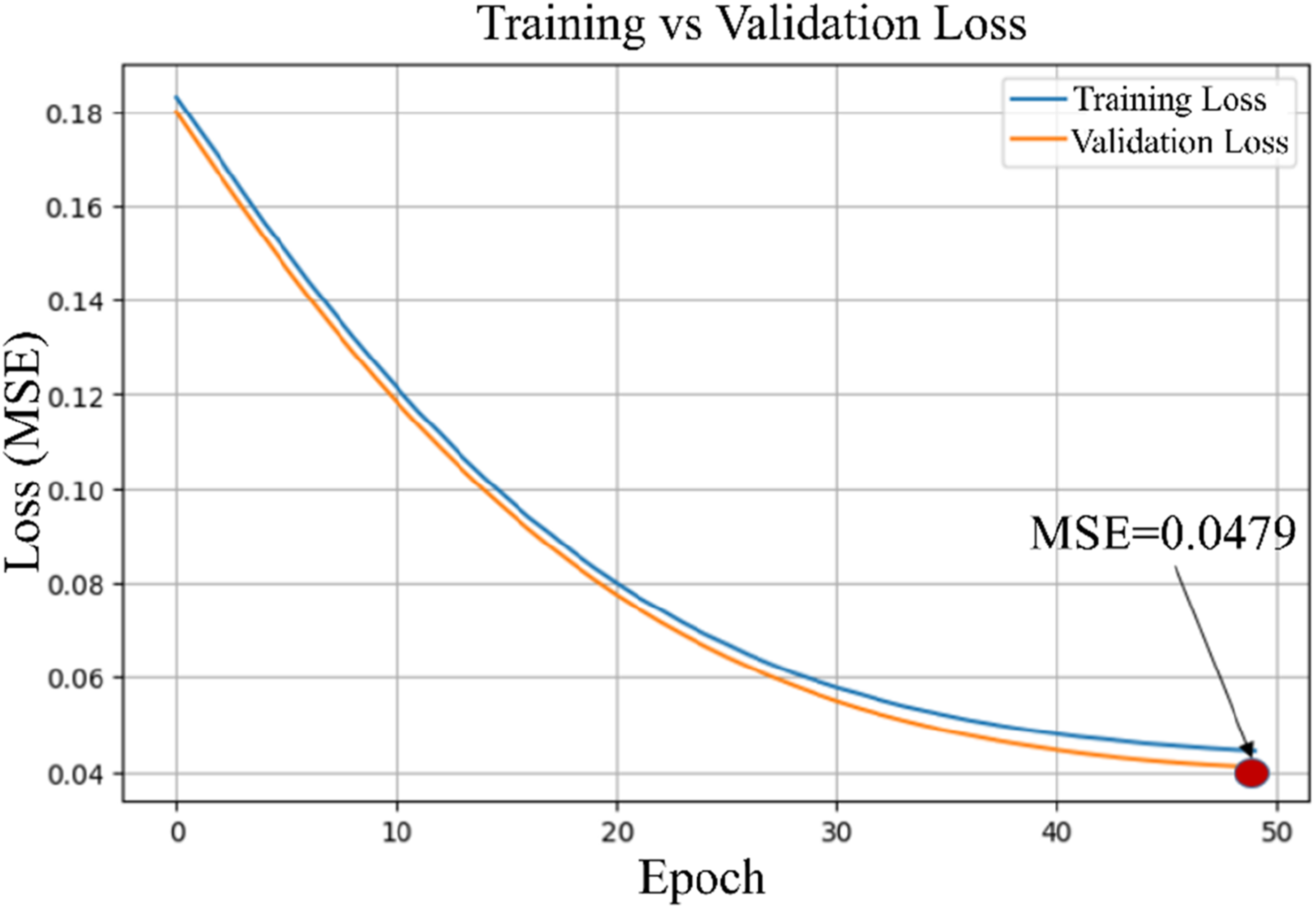

Figure 18(a) shows the PSNR values for the test dataset, which is 20% of the total data. For 12 samples, three samples were used for testing, with the PSNR values for the corresponding reconstructed samples ranging between 13.30 dB and 14.81 dB, as illustrated in Figure 18(a). Normally, for good quality image reconstruction with minimal distortion and noise, a PSNR value of more than 20 dB is considered. The PSNR values are significantly lesser in this study, which is due to a limited dataset size that hinders the model in effectively learning and generalizing the complex features of the images. This limitation leads to an indication that an improved feature extraction capability of the model could be accomplished by increasing the number of training samples, thus improving the overall reconstruction fidelities with higher PSNR values and better visual quality.

Figure 18.

Validation metrics of ANN (a) PSNR, (b) SSIM.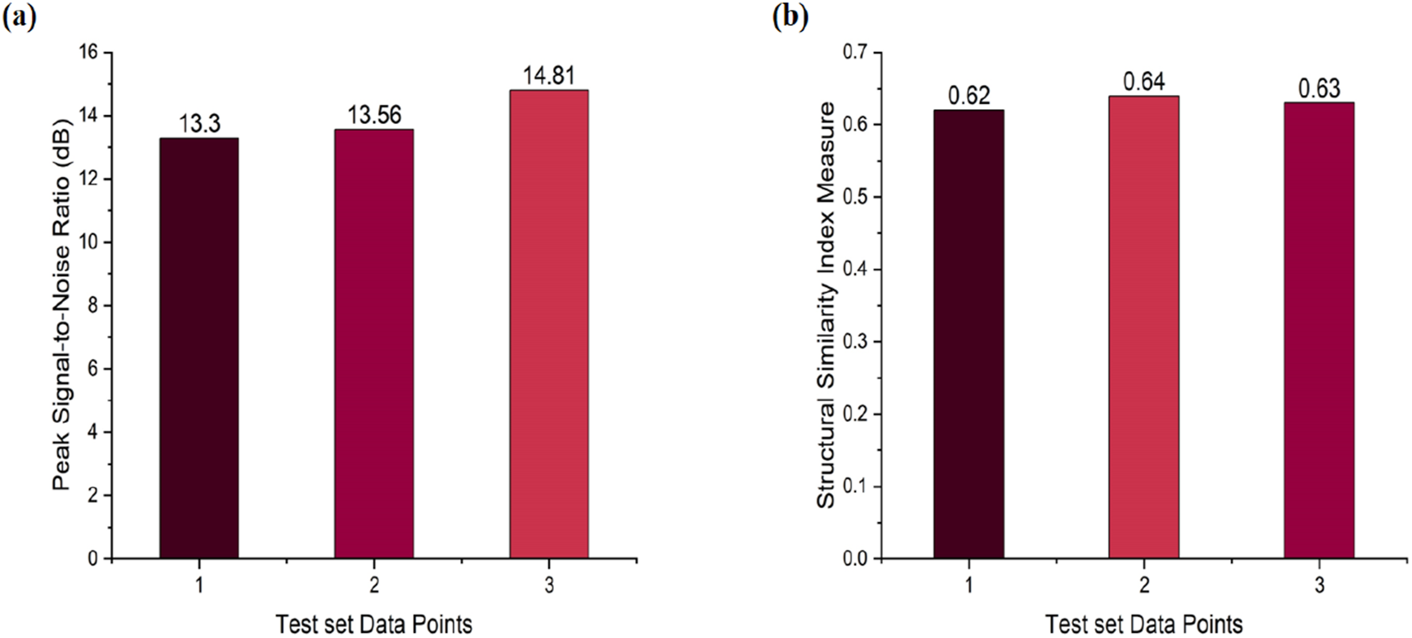

Figure 18(b) shows the calculated SSIM values for the test dataset. SSIM gives the perceived similarity between the reconstructed and original images based on the consideration of structural information, contrast, and luminance. As shown in the figure, the maximum SSIM value achieved is 0.64, and the minimum is 0.62, indicating that all reconstructed test images have SSIM values greater than 0.60. An SSIM value closer to 1.0 implies a high degree of similarity between the predicted and original images. In this case, although the SSIM values do not reach very high levels, they fall within a moderate similarity range, suggesting that the ANN model has preserved key structural and visual features of the original experimental images. The achieved SSIM values indicate that the reconstructed outputs are moderately close in quality to the real images, affirming the model’s capability in generating structurally consistent predictions is moderate.

Figure 19 presents a visual comparison between the experimental and predicted damage area images generated using the ANN model. The visual fidelity of the predicted image is consistent with the quantitative evaluation metrics PSNR and SSIM, both yielding moderate values. These metrics quantitatively assess image quality; PSNR evaluates pixel-level differences, while SSIM calculates structural and perceptual similarity. From this, one may infer that while the ANN model captures the overall structure of the damage region reasonably well, the finer details are not accurately reproduced. Specifically, the central region of damage in the predicted image is distinctly identified, indicating that the ANN has learned the approximation of the core features of the damage pattern. However, the outer peripheral features of the damage area are blurred or missing. This discrepancy would suggest a limitation of the model on generalizing complex spatial patterns beyond the dominant features.

Figure 19.

Comparison of experimental damage image output with predicted damage area image output of ANN model.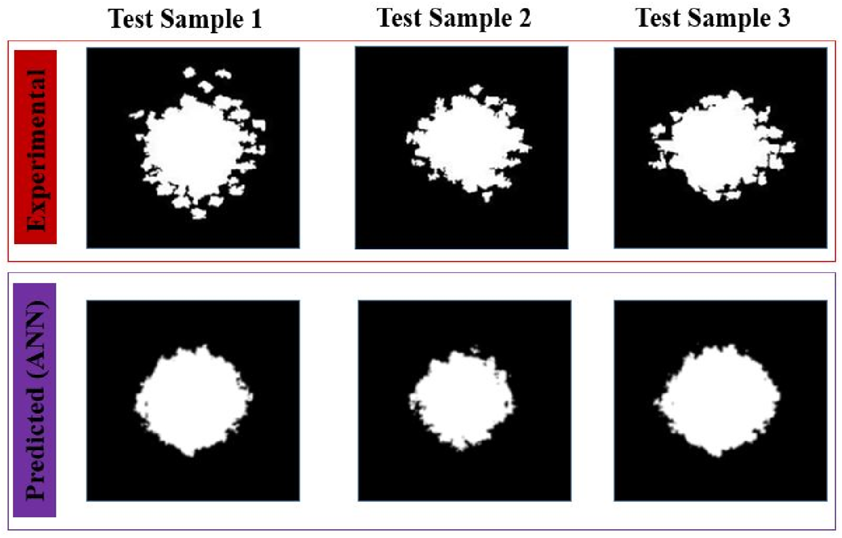

This is principally due to the limited size of the training dataset. In most neural networks, especially in tasks involving the prediction or reconstruction of images, large and diverse datasets are required for effective learning of both global and local features. If the dataset is small, the model might over-fit to dominant patterns in it and lose subtler, less frequent damage characteristics. Increasing the dataset with more representative and high-quality samples would likely improve the learning capability of the model and make it possible to achieve more accurate and detailed predictions of the damage areas in future versions.

Conclusion

The DA in NSPs was analyzed with regression and ANN models through both quantitative metrics and a visual comparison. Regarding the scalar estimation, the regression models have well-predicted the numerical values of the damage area, while the ANN model has satisfactorily reconstructed the area of damage from a more visual point of view, catching the main central features but losing the finer details of the periphery. The key findings are as follow:

(1) While the DT model was the best model in terms of DA of NSPs prediction with an R² of 0.99, its residual analysis indicated a significant overfitting issue, with zero residuals in training and very poor generalization capability on unseen data. However, the PR model (R² = 0.94) had more consistent performance and presented only minor overfitting as evidenced from slightly scattered test residuals around the zero line. Although its accuracy was marginally lower, it strikes a better balance in model fit and generalization capability. Overall, the PR model can be said to be more reliable in predicting DA of NSPs due to greater stability and reduced risk of overfitting than that in DT models.

(2) Altogether, the analyses of Cρ and LOOCV have established that the PR model (Degree = 2) has strong predictive capabilities for DA with limited overfitting. The minor decrease of the value of Cρ from 0.96 in training to 0.90 in test conditions, and the convergence of LOOCV R² values around 0.95, indicate that the model maintains stability in both accuracy and generalization even with a small data size. Minor performance fluctuations arise in the face of small sample sensitivity; overall, this trend shows the PR model captures the underlying data pattern very well and yields sound predictions that could be further fine-tuned through regularization or by expanding the number of training examples.

(3) From the SHAP, feature importance, and partial dependence analyses, it can be observed that IE is the primary factor influencing DA, while NCP has a secondary but beneficial effect. The model predictions indicate that DA increases noticeably with higher IE, whereas increasing NCP tends to reduce DA due to improved interfacial bonding and composite stiffness. Thus, this analysis confirms that while increasing impact energy significantly enlarges the damaged area, an increase in nano clay content improves the resilience of composites through reduced damage severity.

(4) Adding 2% nano-clay to aluminium honeycomb sandwich panels reduced the damage area by about 41% at 10 J, 37% at 20 J, 32% at 30 J, and 23% at 40 J, while only a marginal improvement was obtained by further increasing the nano-clay to 4%, indicating the optimal reinforcement level to be 2%. This improvement is attributed to the high-aspect-ratio nano-clay and their interfacial bonding that improve stress distribution and hinder crack propagation. At 2% NCP, the reduction in damages decreased from 41% at 10 J to 23% at 40 J, confirming impact energy as the dominant factor, which is in agreement with SHAP and feature importance analysis.

(5) The ANN model showed effective learning over the course of 50 epochs, with a gradual decrease in both training and validation losses, reaching a low final MSE of 0.0479, which indicates predictive accuracy and stable generalization. It predicted the area of damage, reconstructing key regions such as the central impact zone, although some finer peripheral features were not as sharply delineated. Quantitative evaluations based on PSNR (13.30–14.81 dB) and SSIM (0.62–0.64) reflected the image fidelity with limited visual clarity and structural similarity. These results demonstrate that the ANN can generalize effectively within the available data, but the relatively small dataset modestly constrains the network from learning more detailed and complex spatial features. Future work involving a larger and more diverse dataset is foreseen to further enhance the model’s reconstruction quality and overall predictive performance.

In future studies, the dataset will be broadened to include more representative and varied samples in order to enhance the capability of the model in describing complex damage patterns. Moreover, other deep learning models such as CNN, U-Net, ResNet, and DenseNet will be implemented with the aim of accomplishing high prediction accuracy and image reconstruction quality. It is realized that these models have remarkable performance in extracting spatial features and analyzing images in great detail. The integration of the techniques discussed is expected to greatly enhance the fidelity of predictions for areas of damage.

Footnotes

ORCID iDs

Saravanamuthukumar Ponraj

Jayaram Radhakrishnan Santhi

Author contributions

Saravanamuthukumar P: Writing– original draft, ML Model validation, Methodology, Data curation, Conceptualization. Ahmad Baharuddin Abdullah: Writing– original draft, Validation, Formal analysis, Data curation. R S Jayaram: Writing– original draft, Resources, Data curation. Krishnamoorthy Ramalingam: Validation, Formal analysis, Data curation.

Funding

The authors received no financial support for the research, authorship, and/or publication of this article.

Declaration of conflicting interests

The authors declared no potential conflicts of interest with respect to the research, authorship, and/or publication of this article.

Data Availability Statement

The datasets used and/or analysed during the current study available from the corresponding author without any restriction.*

Declaration of Generative AI and AI-Assisted Technologies in the Writing Process

During the preparation of this work, the authors utilized Copilot to enhance language and readability. After employing this tool/service, the authors thoroughly reviewed and edited the content as necessary and assume full responsibility for the final publication.

References

Wang

, et al. Lightweight research in engineering: a review. Appl Sci 2019; 9: 5322. https://doi.org/10.3390/app9245322

Hassan

Saeed

. Advancements and applications of lightweight structures: a comprehensive review. Discover Civil Eng 2024; 1: 47. https://doi.org/10.1007/s44290-024-00049-z

Sun

Chen

Zhu

, et al. Lightweight hybrid materials and structures for energy absorption: a state-of-the-art review and outlook. Thin-Walled Struct 2022; 172: 108760. https://doi.org/10.1016/j.tws.2021.108760

Taub

Luo

. Advanced lightweight materials and manufacturing processes for automotive applications. MRS Bull 2015; 40: 1045–1054. https://doi.org/10.1557/MRS.2015.268

Phiri

Rangappa

Siengchin

, et al. Advances in lightweight composite structures and manufacturing technologies: a comprehensive review. Heliyon 2024; 10: e39661. https://doi.org/10.1016/j.heliyon.2024.e39661

Singh

Srivastawa

Jana

, et al. Advancements in lightweight materials for aerospace structures: a comprehensive review. Acceleron Aerospace J 2024; 2: 173. https://doi.org/10.61359/11.2106-2409

Rajkumar

. Strength and stiffness characteristics of A3003 aluminum honeycomb core sandwich panels. Mater Today Proc 2020; 37: 1140–1145. https://doi.org/10.1016/j.matpr.2020.06.348

Jia

Liu

, et al. Response of aluminium honeycomb sandwich panels under combined shock and impact loading: experimental and numerical investigations. Thin-Walled Struct 2023; 193: 111256. https://doi.org/10.1016/j.tws.2023.111256

Yahaya

Ruan

, et al. Response of aluminium honeycomb sandwich panels subjected to foam projectile impact - an experimental study. Int J Impact Eng 2015; 75: 100–109. https://doi.org/10.1016/J.IJIMPENG.2014.07.019

10.

Jayaram

Nagarajan

Vinod Kumar

. Low velocity impact and compression after impact behaviour of polyester pin-reinforced foam filled honeycomb sandwich panels. J Sandw Struct Mater 2022; 24(1): 157–173. https://doi.org/10.1177/1099636221998180

11.

Shi

Zhou

Zhang

, et al. In-plane compressive response of composite sandwich panels with local-tight honeycomb cores. Compos Struct 2023; 314: 116970. https://doi.org/10.1016/j.compstruct.2023.116970

12.

Abid Allah Hamza

Al-Fatlwe

Talib

. Experimental and numerical study of effecting core configurations on the static and dynamic behavior of honeycomb plate with aluminum material. Def Technol 2023; 39: 177. https://doi.org/10.1016/j.dt.2023.11.016

13.

Rao

Sarwade

, et al. Bending behavior of aluminum honey comb sandwich panels. Int J Eng Adv Technol 2012; 1: 268–272.

14.

Zhang

Guo

, et al. Dynamic mechanical behaviour and energy absorption of aluminium honeycomb sandwich panels under repeated impact loads. Ocean Eng 2020; 219: 108344. https://doi.org/10.1016/j.oceaneng.2020.108344

15.

Zhang

, et al. Ballistic impact behaviors of aluminum alloy sandwich panels with honeycomb cores: an experimental study. J Sandw Struct Mater 2018; 20: 861–884. https://doi.org/10.1177/1099636216682166

16.

Yan

Wang

Pan

, et al. Stability and failure of the edge- closed honeycomb sandwich panels with face/core debonding. Appl Sci 2020; 10: 7457.

17.

Wei

Gao

, et al. Bending characteristics of allcomposite hexagon honeycomb sandwich beams: experimental tests and a three-dimensional failure mechanism map. Mech Mater 2020; 148: 103401.

18.

Jamshidi

Azhari

Amoushahi

. Free vibration of plates of various shapes with intermediate point supports by the Hp-Cloud method and lagrange multiplier. Int J Struct Stabil Dynam 2016; 16(09): 1550055. https://doi.org/10.1142/S0219455415500558

19.

Hosseini

Amoushahi

Azhari

. Nonlinear effect of low-velocity impact on tapered laminated composite structures using spline finite strip method. Structures 2022; 39: 739–764. https://doi.org/10.1016/j.istruc.2022.03.051

20.

Teng

Zhang

, et al. The use of pre-hole Z-pinning (PHZ) method to improve the impact resistance and post-impact flexural performance of composite skin/stringer joints. Thin-Walled Struct 2022; 180: 109909. https://doi.org/10.1016/j.tws.2022.109909

21.

Zhang

Van Hoa

, et al. Effect of Z-pinning on fatigue crack propagation in composite skin/stiffener structures. J Compos Mater 2018; 52: 275–285. https://doi.org/10.1177/0021998317710708

22.

Cartié

Dell’Anno

Poulin

, et al. 3D reinforcement of stiffener-to-skin T-joints by Z-pinning and tufting. Eng Fract Mech 2006; 73: 2532–2540. https://doi.org/10.1016/J.ENGFRACMECH.2006.06.012

23.

Potluri

Kusak

Reddy

. Novel stitch-bonded sandwich composite structures. Compos Struct 2003; 59: 251–259. https://doi.org/10.1016/S0263-8223(02)00087-9

24.

Kim

Choi

. Failure strength of composite T-joints prepared using a new 1-thread stitching process. Compos Struct 2017; 178: 225–231. https://doi.org/10.1016/J.COMPSTRUCT.2017.07.003

25.

Morano

Wagih

Alfano

, et al. Improving performance of composite/metal T-joints by using corrugated aluminum stiffeners. Compos Struct 2022; 307: 116652. https://doi.org/10.1016/j.compstruct.2022.116652

26.

Jayaram

Nagarajan

Vinod Kumar

. Compression and low velocity impact response of sandwich panels with polyester pin-reinforced foam filled honeycomb core. J Sandw Struct Mater 2019; 21(6): 2014–2030.

27.

Ferdous

Manalo

Aravinthan

. Bond behaviour of composite sandwich panel and epoxy polymer matrix: taguchi design of experiments and theoretical predictions. Constr Build Mater 2017; 145: 76–87. https://doi.org/10.1016/J.CONBUILDMAT.2017.03.244

28.

Anbusagar

Palanikumar

Giridharan

. Study of sandwich effect on nanoclay modified polyester resin GFR face sheet laminates. Compos Struct 2015; 125: 336–342.

29.

Bozkurt

Kaya

Tano˘glu

. Mechanical and thermal behavior of non-crimp glass fiber reinforced layered clay/epoxy nanocomposites. Compos Sci Technol 2007; 67: 3394–3403.

30.

Prasanth

Sahaya Raj

Jappes

, et al. Study of matrix modifications by NC on the mechanical properties of AA3003 honeycomb sandwich panels. Proc IME C J Mech Eng Sci 2022; 236(14): 7974–7983.

31.

Ong

. Accelerating materials science with high-throughput computations and ML. Comput Mater Sci 2019; 161: 143–150. https://doi.org/10.1016/J.COMMATSCI.2019.01.013

32.

Mobarak

Mimona

Islam

, et al. Scope of ML in materials research—a review. Appl Surf Sci Adv 2023; 18: 100523. https://doi.org/10.1016/j.apsadv.2023.100523

33.

Chen

. ML for composite materials. MRS Commun 2019; 9: 556–566. https://doi.org/10.1557/mrc.2019.32

34.

Dinic

Singh

Dong

, et al. Applied ML for developing next‐generation functional materials. Adv Funct Mater 2021; 31: 2104195. https://doi.org/10.1002/adfm.202104195

35.

Osa-uwagboe

Udu

Ghalati

, et al. A ML-enabled prediction of damage properties for fiber-reinforced polymer composites under out-of-plane loading. Eng Struct 2024; 308: 117970. https://doi.org/10.1016/j.engstruct.2024.117970

36.

Dhanesh

Nagarajan

Vinod Kumar

, et al. Quantitative assessment of impact damage in stitched foam-filled aluminium honeycomb sandwich panels by experimental and ML methods. Polym Compos 2024; 45(15): 13663–13675. https://doi.org/10.1002/pc.28726

37.

Ranjbar-Roeintan

Ahmadian

Soleymani

. Predicting low-velocity impact on the CNTs-reinforced plate using ML models. World J Eng 2024; 22: 1290.

38.

Kamarian

Teimouri

Alinia

, et al. ML for bending behavior of sandwich beams with 3D‐printed core and natural fiber‐reinforced composite face sheets. Polym Compos 2024; 45(4): 3043–3054.

39.

Qing

. Data-driven prediction on critical mechanical properties of engineered cementitious composites based on ML. Sci Rep 2024; 14: 15322. https://doi.org/10.1038/s41598-024-66123-9

40.

Parra

Ferreira

Díaz

, et al. Supervised ML models for mechanical properties prediction in additively manufactured composites. Appl Sci 2024; 14(16): 7009. https://doi.org/10.3390/app14167009

41.

Vanerio

Guagliano

Bagherifard

. ML image-based analysis for bead geometry prediction in fused granulate fabrication for large format additive manufacturing. NPJ Adv Manuf 2025; 2(1): 8.

42.

Manujesh

Prajna

. Damage detection and classification for sandwich composites using ML. Mater Today Proc 2022; 52: 702–709.

43.

Viotti

Gomes

. Delamination identification in sandwich composite structures using ML techniques. Comput Struct 2023; 280: 106990.

44.

Rautela

Senthilnath

Monaco

, et al. Delamination prediction in composite panels using unsupervised-feature learning methods with wavelet-enhanced guided wave representations. Compos Struct 2022; 291: 115579.

45.

Mehrpouya

Gisario

Nematollahi

, et al. The prediction model for additively manufacturing of NiTiHf high-temperature shape memory alloy. Mater Today Commun 2021; 26: 102022.

46.

Wen

Zhang

Wang

, et al. Machine learning assisted design of high entropy alloys with desired property. Acta Mater 2019; 170: 109–117.

47.

Zhang

. Transformation temperature predictions through computational intelligence for NiTi-based shape memory alloys. Shape Mem Superelasticity 2020; 6(4): 374–386.

48.

Tian

Lauria

, et al. Recent advances on loss functions in deep learning for computer vision. Neurocomputing 2022; 497: 129–158. https://doi.org/10.1016/j.neucom.2022.04.127

49.

Tanchenko

. Visual-PSNR measure of image quality. J Vis Commun Image Represent 2014; 25(5): 874–878.

50.

Deshpande

Ragha

Sharma

. Video quality assessment through PSNR estimation for different compression standards. Indones J Electr Eng Comput Sci 2018; 11(3): 918–924.

51.

Bovik

. Three-component weighted structural similarity index. In Image quality and system performance VI. SPIE, 2009, Vol. 7242, pp. 252–260.

52.

Sara

Akter

Uddin

. Image quality assessment through FSIM, SSIM, MSE and PSNR—a comparative study. J Comput Commun 2019; 7(3): 8–18.

53.

Schober

Boer

Schwarte

. Correlation coefficients: appropriate use and interpretation. Anesth Analg 2018; 126: 1763–1768.

54.

DiagnosticOn

. Pearson's correlation coefficient. N Z Med J 1996; 109(1015): 38.

55.

Berggren

. Coefficients of determination measured on the same scale as the outcome: alternatives to R² that use standard deviations instead of explained variace. Psychol Methods 2024, Advance online publication.

56.

Nordin

Zainol

Noor

, et al. An explainable predictive model for suicide attempt risk using an ensemble learning and Shapley Additive Explanations (SHAP) approach. Asian J Psychiatry 2022; 79: 103316. https://doi.org/10.1016/j.ajp.2022.103316

57.

Oral

Maddah

Yıldırım

. Predictive modeling and SHAP (SHapley Additive ExPlanations) analysis for enhancing natural dye‐sensitized solar cell performance. Sol RRL 2024. https://doi.org/10.1002/solr.202400432