






Abstract
Background
T-wave alternans (TWA) refers to variations in the ventricular repolarization pattern observed on the ECG, which has been associated with cardiac instability and an increased risk of sudden cardiac death. Recently, machine learning (ML) methods have been developed for TWA detection, but their black-box nature limits interpretability.
Objectives
To address this gap, we propose manifold learning (MnL) to enhance the explainability of these learning models while maintaining TWA detection effectiveness.
Methods
We fine-tuned nonlinear dimension reduction techniques such as Uniform Manifold Approximation and Projection (UMAP), Isometric Mapping (Isomap), and autoencoders (AE) in combination with ML methods, namely K-nearest neighbors (KNN), random forest (RF), and neural networks (NN). Performance was evaluated using mean and standard deviation across patient-wise permutations.
Results
In the design stage, the AE-based NN effectively retained essential discriminative information (F1-score 92.1 ± 2.4 %). MnL-generated spaces consistently revealed that misclassifications primarily lie close to the decision boundary and are predominantly associated with lower TWA voltages, which are more dispersed within the space. For ambulatory TWA detection, Isomap combined with RF and the AE-based NN achieved performance comparable to using the complete set of features derived from established TWA analysis methods (F1-score 78.5 ± 6.4 % and 77.9 ± 5.4 %, respectively), including spectral, time-domain, and correlation-based descriptors. The latent space visualization shows that predictions that ultimately become detections are located farther away from the decision boundary.
Conclusion
MnL-generated spaces provide valuable insights into how classification models differentiate between TWA and non-TWA instances, as well as the patterns in TWA event amplitudes. This approach helps bridge the gap between performance and transparency, supporting more clinically reliable TWA detection.
Keywords
1. Introduction
Cardiovascular disease is among the leading causes of death globally, where sudden cardiac death (SCD) stands for, approximately, half of all cardiovascular deaths. Although it has been proven that SCD incidence is declining, the proportion of SCD risk with respect to the overall cardiovascular death may have increased. 1 Several electrocardiographic indices have been proposed to stratify SCD risk, where T–wave alternans (TWA) is among them.2-5 TWA refers to micro–volts variations of the ventricular repolarization section of the surface ECG (ST–T segment) on an every–other–beat basis. Since alternans are not visible to the naked eye, computational means are required for its identification. 6
Heart rate was found to be a modulator of TWA, so, traditionally, atrial pacing was the means of accelerating the heart rhythm for TWA detection.7,8 In parallel, exercise testing was proven to be equivalent and more convenient for being less invasive and harmful,9,10 though still supervised by clinicians. Currently, research focuses on ambulatory recording detection using methods capable of tracking the signal in real time to trigger alerts, or perform off–line analysis of cardiac risk. This acquisition method is very convenient because it can be used with a larger population and it is compatible with wearable ECG systems. In contrast, it provides an unstabilized signal exposed to changing conditions due to its ambulatory nature. To accurately capture the dynamic changes in the ECG, TWA detection methods should operate with the shortest possible windows. This allows them to identify transient TWA episodes that may not occur frequently and to handle a wide range of alternans amplitudes.
The fields of discrete–time signal processing as well as the detection and estimation theory have been exploited to develop methods for alternans identification. The Spectral Method (SM), 11 which relies on the Fourier analysis of time–series in the heartbeat domain, and the Laplacian Likelihood Ratio (LLR) method, 12 which estimates the maximum likelihood under Laplacian noise assumption, are two very efficient methods. Other approaches employ the Wavelet Transform, 13 Matched Filter, 14 Principal Component Analysis, 15 Empirical Mode Decomposition, 16 or Bootstrap resampling. 17 In the time domain, the Correlation Method (CM) 18 uses an alternans index based on the cross correlation and the Modified Moving Average (MMA) 19 applies non–linear filtering. Machine learning (ML) has also been used for this purpose, thanks to the data ensemble that we designed in Ref. 20. We configured a repository of control ECGs (signals without TWA) taken from publicly available databases to obtain labeled datasets by inserting TWA. We developed this signal model because other more simplistic based on synthetic ECGs, and used in most approaches as a surrogate for non–existent annotated databases, do not explain how detectors operate in real-world environments. 21 With this model, we capture both the structural variability of the signal and the waveform difference among patients. The methodology to assemble the repository is easy to replicate and the probability of false alarm has been found negligible: 9.7 ⋅ 10−7, 3.2 ⋅ 10−5, and 4.11 ⋅ 10−4 with the LLR, the SM, and the CM, respectively, confirming its validity.
In the initial attempt to characterize TWA with ML, we proved in Ref. 20 that learning–based models can detect subtle alternans of 35 μV in 32–beat long ECG excerpts using a set of 3 features (F1-score 0.89 with Decision Trees). Subsequently, we increased the set of variable up to 14, chosen among representative TWA signal processing methods and provided two main advances. 22 First, we applied the same training procedure, but over smaller ECG–beat blocks (30–beats) and used a wide range of alternans amplitudes (20 to 100 μV) instead of a single one to train the ML models. Second, we deployed the models in real working conditions, where the contextual situation is far different from the idealized training scenario. Thus, we showed that tracking short and sporadic TWA events in ambulatory records with ML models is feasible with nice performance (F1-score 0.80 with Random Forest (RF)). Also, compared to standalone signal processing techniques like SM and LLR (F1-score 0.78 and 0.66, respectively), ML-based models demonstrated superior detection performance due to their increased sensitivity to true TWA events and reduced false negative rate.
A limitation of learning methods is that we must trust the predictions without understanding why they are made, as these systems operate as black boxes, where the internal mechanisms are not disclosed. Moreover, as long as a machine does not provide any explainability about its behavior, the confidence of clinical practitioners can crumble, which is one of the reasons that hinders the transfer of this technology to clinical routine. 23 Currently, there is a growing interest among physicians in understanding the knowledge extracted by machines and the potential significance of relevant patterns in AI–based disease diagnostic systems before fully trusting them. 24 The more decisions of a machine impact human lives, the more crucial it is for the machine to provide transparency about its decision-making process. 25
In this work, we extend our dataset and the set of ML models, but mainly we propose to use manifold learning (MnL) to improve the explainability of learning models applied to the detection of TWA. Dimensionality reduction techniques facilitate the mapping of high-dimensional data to lower-dimensional representations, making complex data more interpretable. Principal Component Analysis (PCA) has long been the standard for linear dimension reduction, identifying a linear subspace that minimizes reconstruction error when data points are projected onto this space. However, to capture more intricate structures and relationships within the data, nonlinear dimension reduction approaches have emerged. These methods assume that data lie on smooth, nonlinear low-dimensional geometric objects known as manifold embeddings, aiming to preserve the intrinsic geometric information of the data. 26 In this context, we explore state-of-the-art techniques including Uniform Manifold Approximation and Projection (UMAP), Isometric Mapping (Isomap), and autoencoders. Our goal is to leverage these methods to provide a space for interpretability of TWA detection systems. By reducing data dimensionality, we can visualize the data in a three-dimensional space, which aids in understanding the distribution of points and the potential formation of clusters, thereby significantly contributing to the improvement of the models.
The exploration of MnL embeddings for ECG signals is gaining increasing attention as researchers strive to balance high accuracy with interpretability, two aspects that often present a trade-off in ML models. 27 While model-agnostic techniques such as SHAP or LIME provide local explanations, offering insight into why a specific prediction is made, 28 MnL techniques serve a different purpose. They do not aim to explain individual predictions, instead, they reveal the global geometric structure of the data and classifier behavior. 29 This global perspective is particularly beneficial for ECG signals and TWA detection, where understanding the overall data geometry, class separation, and latent clusters can reveal meaningful physiological patterns. Traditional approaches such as PCA, 30 along with more advanced nonlinear methods like UMAP27,30,31 and Isomap, 32 efficiently compress critical information in the latent space of various cardiac conditions such as atrial fibrillation or left ventricular dysfunction, among others. Moreover, a wide range of autoencoders, varying in complexity, have also been employed for this purpose.31,33 These embeddings function as powerful explainability tools, where low-dimensional projections create clusters of similar conditions, effectively demonstrating class separation and revealing underlying patterns in the data.
Particularly, to the best of our knowledge, 34 is the only study that addresses explainability in TWA detection by applying UMAP to project data into a low-dimensional latent space. Their approach differs significantly from ours, as it is fully unsupervised, focuses on electrocardiographic imaging data, and is subject-specific, relying on community detection within the latent space. In contrast, our study employs supervised learning techniques, which allow us to quantitatively assess the effect of dimensionality reduction on detection performance. We also validate our methods on real-world ambulatory ECG data, emphasizing practical clinical applicability. Beyond detection, our aim is to show that improving explainability through MnL does not compromise performance. By expanding the dataset and exploring multiple MnL methods, we seek not only to improve accuracy but also to gain insights into model behavior, such as identifying patterns, understanding decision boundaries, and detecting potential biases. All these differences in data, methodology, and objectives limit direct comparison, while highlighting the distinct contributions of our approach.
The remainder of this paper is structured as follows: Section 2 introduces the dataset and details the feature engineering stage using signal processing techniques. It also addresses the MnL and ML approaches applied in this study for TWA detection. Section 3 outlines the experimental framework, including the design of methods and settings for ambulatory detection. Results are presented in Section 4, followed by a summary of the discussion in Section 5. Finally, conclusions are provided in Section 6.
2. Material and Methods
2.1. Dataset
For this study, we start from the database assembled in Ref. 22 extending it as showed in 3.1. A signal model that incorporates real TWA into real ECG signals without alternans was used. This model has proven to be robust as it accounts for patient and signal variability.17,21,35 The dataset consists of ECG segments, each lasting more than 5 minutes, sourced from MIT–BIH Arrhythmia Database 36 (mitdb), the European ST–T Database 37 (edb), and the MIT–BIH Normal Sinus Rhythm Database (nsrdb), all publicaly available in Physionet. 38 We confirmed that all of them were free of TWA using the SM as gold standard. The repository consist of 574 signals of varying lengths from 30 patients (consult20,22 for further details).
To train our ML models, we randomly select ECG frames consisting of M beats with D beats of overlapping from the 574 signals. Our goal is to develop TWA detectors suitable for ambulatory conditions, so the window size must be as short as possible to minimize the effect of signal variability on the ECG. The selection of these parameter values was thoroughly studied and validated in Ref. 39. Each instance from this set is used as an example for the models. To prevent bias toward patients with longer signals, we ensured a balanced number of instances per signal by limiting the number of instances based on the minimum available across all signals.
The i–th instance is constructed as described in Equation (1), where


The real alternant waveform θ, provided by J. P. Martínez, is incorporated into the ECG instance, randomly selected from 15 available patient waveforms.
12
These TWA events are either stationary or sustained, whereas our previous work
39
presents an example of a non-sustained episode introduced into an ECG segment (see Figure 1). In this equation, ɛ(i)(t), where t = 0, …, L
ɛ
− 1, represents the alternant wave, with L
ɛ
denoting the length of the ST–T complex and L
ɛ
≪ L
i
. The term t
k
is the onset of the ST–T segment for the k-th beat, and t
J
is a zero-mean Gaussian random variable with a standard deviation of 20 ms, which introduces uncertainty to the ST–T onset. In this context, TWA occurs in every other beat: for odd k, no TWA is present (θ(i)(t) = 0), and for even k, the TWA amplitude is defined by α. AE-based NN architecture for MnL. Each square with a cross inside stands for a fully connected layer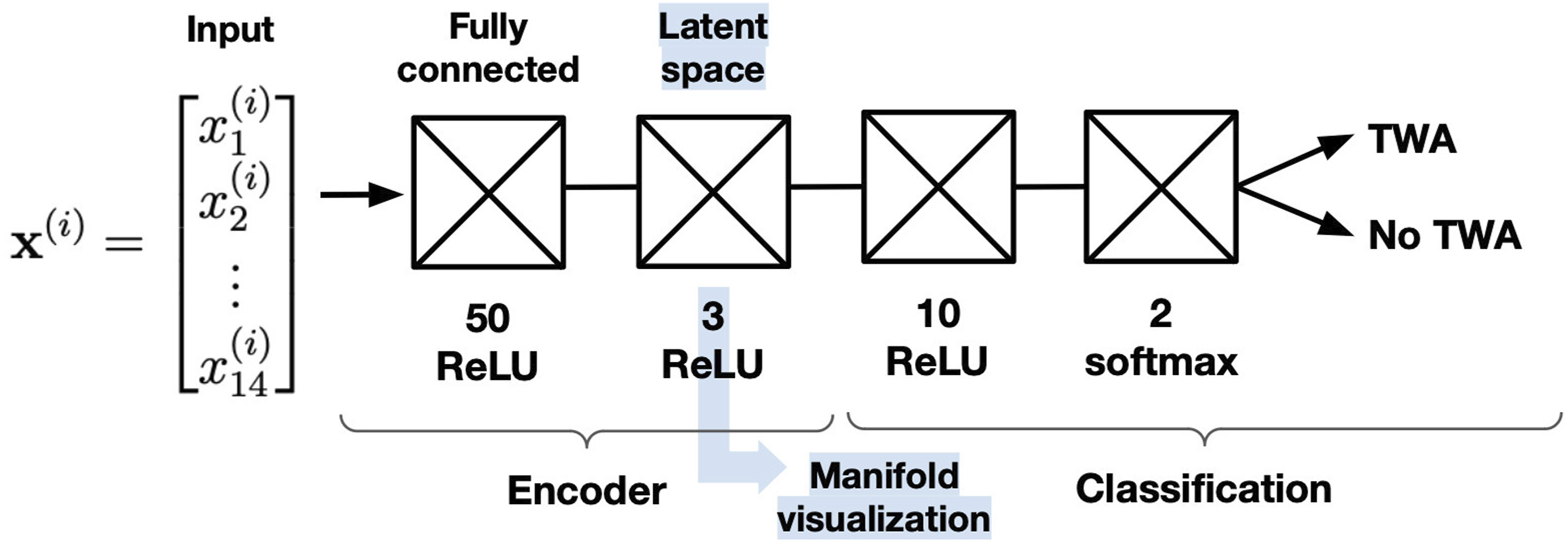
2.2. Feature Set
We use a set of predictors composed of informative descriptors extracted from well-known TWA detection methods, namely, the SM, 40 the MMA, 19 the Time Method (TM), 17 the LLR, 12 the CM 18 , and the Complex Demodulation (CD). 41
All of them extract parameters related to the ventricular repolarization by operating on matrix

Therefore, we extracted a total of 14 features from each ECG frame (Equation (1)) to feed the learning-based algorithms and create the detection models. We selected the K score from the SM (K
score
) and the estimated alternant volage from the MMA
2.3. Dimensionality Reduction
Dimensionality reduction has gained significant attention in recent years for its ability to reduce the number of dimensions in data, while uncovering its intrinsic structure with minimal loss of accuracy and information. Often applied in ML tasks such as classification, clustering and regression, dimensionality reduction helps reduce computational complexity and alleviates the curse of dimensionality. Moreover, it facilitates data visualization by projecting high-dimensional data onto two or three dimensions, making it easier to identify patterns and relationships. Feature selection and feature extraction are the main approaches.
Feature extraction, creates new, independent, and informative features from the original data in an unsupervised manner. Its goal is to capture essential information while reducing redundancy and noise. Methods in this domain fall into two main categories: linear and non-linear approaches. Linear techniques, exemplified by PCA, assume that the intrinsic structure of the data can be well-represented in a lower-dimensional linear subspace. By leveraging principles of linear algebra, these methods condense the data, making them particularly effective for datasets with linear relationships among variables. Conversely, non-linear methods, often referred to as MnL techniques, such as Isomap and UMAP, are designed to handle complex data structures with intricate non-linear relationships. These techniques excel in capturing non-linear manifolds and preserving both local and global patterns in reduced space, offering a more flexible and accurate representation of the data intrinsic geometry. 44 Additionally, autoencoder-based neural networks (AE-based NN) provide another powerful non-linear approach, wherein a neural network learns a compressed, latent representation of the data. This flexibility in network architecture allows AE-based NNs to adapt to specific data complexities and capture fine-grained patterns while reducing dimensionality. 45 We now turn our focus to feature extraction to effectively reduce our dataset dimensionality, thereby enhancing the interpretability of the model behavior.
2.3.1. PCA
PCA, one of the earliest and most widely used techniques in the field, aims to reduce dimensionality by constructing new variables known as principal components, which are linear combinations of the original dataset variables. PCA transforms a high-dimensional input vector into a low-dimensional one by calculating the eigenvectors of the covariance matrix of the centered original inputs. Given the original set of features


The principal components are arranged in descending order of their eigenvalues, with the first component capturing the greatest variance and thus, the most information. Subsequent components account for progressively smaller amounts of variance. By focusing on the first few principal components, one can reduce dimensionality while retaining the most significant information from the dataset. However, despite its widespread use and computational simplicity, PCA has notable limitations. It assumes linear relationships among features, which may not be suitable for datasets with complex non-linear structures, potentially leading to suboptimal dimensionality reduction and loss of crucial information. Moreover, PCA is sensitive to outliers, which can disproportionately affect the principal components and result in biased outcomes. 44
2.3.2. UMAP
UMAP, a non-linear technique introduced by McInnes and Healy, 29 involves two main steps: constructing a fuzzy topological representation of the approximated manifold where the data is presumed to lie, and subsequently optimizing this representation in a low-dimensional embedding.
For the initial high-dimensional graph, a KNN graph is built, in which, for each instance


Through these two parameters, the weight of the edge from instance


UMAP excels in preserving both local and global structures in low–dimensional spaces, making it a powerful tool for visualizing and understanding complex data. One of its strengths is the flexibility in parameter fine-tuning, which allows to fit various datasets and analytical needs. However, UMAP is highly sensitive to the choice of hyperparameters, such as the number of neighbors and minimum distance. Therefore, careful and often time-consuming tuning is needed to achieve optimal results. The number of neighbors parameter strikes a balance between capturing fine-grained details and large-scale manifold features. Smaller values focus on preserving detailed local structures, while larger values prioritize global structures, potentially at the expense of losing some local detail. The minimum distance parameter directly influences the resulting embedding by controlling the construction of the fuzzy simplicial set in the low-dimensional space. Essentially, it determines how closely points can be packed together in the embedding. A larger minimum distance value results in a more spread-out embedding, which helps to emphasize global relationships at the cost of local detail. 29
2.3.3. Isomap
Isomap, short for Isometric Mapping, is a widely utilized non-linear dimensionality reduction technique renowned for its ability to preserve geodesic distances rather than merely Euclidean distances. This feature makes Isomap particularly adept at handling data that resides on non-linear manifolds, effectively capturing the underlying geometric structure of complex, high-dimensional datasets. 49
Three steps are involved in this algorithm: neighborhood graph construction, shortest paths computation, and low-dimensional embedding construction. The first step calculates the distances between instances using the Euclidean distance, such as d(

In summary, Isomap effectively maps high-dimensional data onto lower-dimensional spaces, yet it has several limitations: the choice of neighborhood size can affect the embedding quality, it is computationally intensive for large datasets, and it is sensitive to noise and outliers. Furthermore, Isomap struggles with manifolds that have holes or are not convex, which can result in poor and inaccurate low-dimensional representations.44,51
2.3.4. Autoencoders
Autoencoders, initially developed as lossy data compressors, have evolved into effective non-linear dimensionality reduction techniques. An autoencoder is a type of neural network consisting of two main components: the encoder and the decoder. The encoder compresses input data into a lower-dimensional representation, known as the latent space, while the decoder reconstructs the data from this compressed form to match the original as closely as possible.
Mathematically, given an input vector


In this work, we have implemented an AE-based NN, as done in Ref. 52, integrating a two-neuron classification layer into the traditional autoencoder architecture. This design leverages the latent space, allowing the model to utilize its manifold properties while also performing binary classification. Thus, this model is trained to compress the data into the latent space through the encoder layers and classify it based on the compressed representation. Although this architecture is inspired by traditional autoencoders, it does not include a reconstruction objective. The encoder acts as a supervised bottleneck representation that preserves discriminative information for the downstream task.
Figure 1 illustrates the architecture considered, which has been fine-tuned by selecting several parameters such as the number of layers, neurons per layer, and activation functions. Regularization techniques, namely dropout or L2 weight decay, are also employed to prevent overfitting and improve model robustness. Additional key parameters have also been studied. The number of training examples processed in each iteration, known as the minibatch size, affects training efficiency and stability, while the maximum epochs, representing the number of complete passes through the training dataset, influence the duration and thoroughness of the learning process. These parameters are critical for optimizing the model performance and ensuring that it captures the essential patterns in the data while maintaining versatility when applied to new, unseen data.45,51
2.4. ML Methods
In this stage, the classification process leverages engineered and then reduced features, as detailed in earlier sections, to train learning models. Our goal is to categorize ECG segments from the repository into two categories: no TWA (category 0) and TWA (category 1). We have evaluated multiple methods for this purpose, continuing with methods explored in Ref. 22, namely RF and K-nearest neighbors (KNN). For KNN, similar to the prior study, we optimized the number of neighbors across a range of 2 to 20. For RF, we performed fine-tuning on parameters such as minimum leaf size and number of splits, varying from 15 to 20, and number of trees, ranging from 1 to 15, using a grid search approach. This rigorous parameter optimization aims to identify configurations that achieve the best classification performance for our dataset.
Additionally, we have incorporated MultiLayer Perceptron (MLP) in this study. MLP is a type of artificial neural network that utilizes layers of neurons to establish a nonlinear mapping between input and output vectors. It employs a backpropagation algorithm to optimize weight values based on gradients. Key parameters, including the number of layers and the number of neurons per layer, were carefully optimized to maximize performance. A range of values from 10 to 50 neurons was explored across different layer configurations. 20
3. Experimental Framework
Previous studies have highlighted the challenge of applying methods designed for short-term analysis to long-term ECG signals, prompting an exploration of optimal window sizes as seen in prior work. 39 Based on our findings, a window size of M = 30 was determined to yield favorable results. Furthermore, the practical applicability of these trained models was successfully demonstrated in real-life scenarios involving ambulatory recordings featuring realistic TWA episodes. Specifically, simulations were conducted across alternant voltages ranging from 20μV to 100μV in 10μV increments, mirroring practical conditions.
In this study, our primary goal remains consistent with our existing pipeline, which is to accurately detect TWA episodes. However, we are introducing a MnL stage to deepen our understanding of how our models behave. By continuously evaluating model performance through this lens of interpretability, we can gain insights into both their strengths and weaknesses, allowing us to pinpoint areas for improvement and refine our methodologies accordingly.
3.1. Design Stage
For the model training we feed the 14 features obtained from the feature engineering process into the learning models. TWA is introduced randomly in half of the instances for each patient and consistently across the entire 30-beat window. Additionally, the alternant voltages, ranging from 20μV to 100μV, are evenly distributed within the signals, ensuring the learning models are capable of detecting various episodes effectively. This setup follows the clinically inspired protocol introduced in our previous study, 22 with voltages and durations designed to reflect plausible physiological manifestations of TWA. To mitigate the risk of overfitting to synthetic patterns, we deliberately avoid fixed templates or repetitive insertion points. Instead, TWA episodes are randomized across patients and permutations, ensuring diversity and realism in the training data.
In a supervised classification problem like ours, having a properly diverse and representative dataset is essential for enhancing the model ability to generalize to unseen data. To achieve this, in this work we have expanded our training set by adopting an overlapping approach within the instances in this work. Each window now spans 30 beats, with a 5-beat advancement for the subsequent window, resulting in an overlap of 25 beats. This adjustment allows us to consider 288 windows per patient, determined by the patient with the fewest available windows, compared to the 40 windows considered in our previous study. Consequently, our training dataset now includes a total of 8640 instances, marking an increase of over 7 times from our previous set. This change not only enhances the training of the learning models, making them more robust with a larger number of instances to learn from, but also mirrors the approach used for inline TWA detection in ambulatory recordings. Therefore, the models will experience consistent conditions across both experiments. In essence, the expanded dataset boosts the models capacity to learn, generalize and adapt to different contexts and conditions, ultimately enhancing overall performance and reliability.
In this work, we divide the patients into six uniform groups for a test set permutation, following the same procedure as in Ref. 22 , but increasing the number of instances per group from 200 to 1,440. Each group is used once as the test set and the other five for training. To prevent any window-level leakage, all overlapping windows from each patient remain within the same group, as window generation is performed after patient assignment. This strategy assesses generalization, strengthens statistical validity, and reduces the risk that results arise from random chance or specific data patterns. Within the training groups, we tune model hyperparameters using the F1-score, fitting on four groups and validating on one chosen at random. This yields a distinct model for each permutation, tested on its corresponding test group, and we report the mean and standard deviation across permutations to measure performance consistency.
As discussed in Section 2.3, MnL techniques, including UMAP, Isomap, and AE-based NN, are sensitive to their hyperparameter configurations. To ensure robust performance despite data variability and noise, we conducted comprehensive hyperparameter tuning to identify optimal settings across conditions. In this study, we conducted a hyperparameter tuning process for these three MnL techniques, while PCA was kept at its default configuration, given its simplicity and limited tuning requirements. To systematically evaluate the impact of hyperparameter settings on the performance of these methods, we first optimized the parameters of the ML models, namely KNN, RF, and MLP, using PCA-transformed data. This established a strong baseline configuration for the ML models. Subsequently, we explored a range of hyperparameter values for UMAP and Isomap, evaluating their performance within each of the three ML models. The optimal hyperparameter configuration for both UMAP and Isomap was determined based on their performance across these models. Once the best configurations were identified for each of the ML models, these were re-optimized by fitting them to the data transformed using the selected UMAP and Isomap settings. This two-stage tuning strategy, supported by cross-validation, ensured that the MnL techniques were fine-tuned for the specific data transformations, improving the overall effectiveness of the subsequent ML model evaluations.
To fine-tune the dimensionality reduction methods, we systematically explored the hyperparameter space for each technique. For UMAP, we varied the number of neighbors between 10 and 60 and the minimum distance from 0.1 to 0.9. For Isomap, we tested neighbor values from 10 to 30. For the AE-based NN, we evaluated several architectural configurations before selecting the final design shown in Figure 1. The model consists of a fully connected layer with 50 neurons, followed by a 3-dimensional bottleneck, and a post-bottleneck fully connected layer with 10 neurons feeding a 2-unit softmax classifier. All hidden layers use batch normalization, leaky-ReLU activations, and dropout (0.2). Training is performed end-to-end using a single cross-entropy classification loss (no reconstruction loss), Adam optimization, L2 regularization (λ=0.001), batch size 512, and 1000 epochs.
Finally, to evaluate the performance of the design stage, we use several metrics. Accuracy measures how often the model correctly classifies an ECG frame as either TWA or not. Recall evaluates the proportion of TWA cases that are correctly identified, while precision indicates the correctness of the positive classification results. Finally, the F1-score combines both recall and precision into a single metric to provide a balanced assessment. 22
3.2. TWA Detection on Ambulatory Recordings
For real-time detection of sporadic TWA episodes in ambulatory settings, we apply a short-term sliding window to the ECG signal to assess the presence of TWA. In this section, we shift focus to the long-term analysis of the 574 ECG signals, denoted as p(t), in contrast to the short-term instances defined in Equation (1), which were previously employed for system design and training. The ECG model incorporating TWA episodes is described in Equation (13), where θ(t) (previously defined in Equation (2)) represents the stationary alternant waveform. However, in this case, instead of iterating over M beats in an instance, we iterate over N
h
, which denotes the total number of heartbeats in each signal. Example of inline TWA detection on signal 16265 from nsrdb using the AE-based NN. The model predictions (thin blue line) and the final detections (thick green line) corresponding to the TWA episodes (thick horizontal black line) are illustrated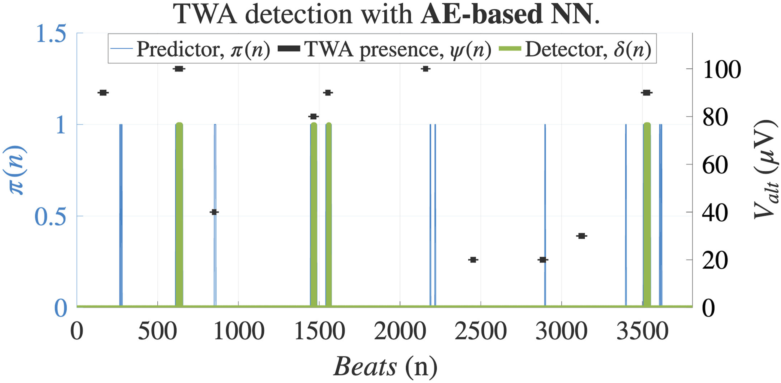


To make predictions about TWA presence, a sliding square window is applied to the signal, represented as P
w
(t, τ) = w(τ)P(t− τ), where the window size M is 30 beats. Signal processing-based methods and ML models generate predictions from this window. However, the former yields continuous-valued predictions, while the latter provides binary decisions. A prediction π(n) is made from the output

Lastly, TWA episodes may appear as sporadic events in long-term ECG signals. However, the learning models were trained under balanced conditions to ensure optimal performance. As a result, the predictions are prone to a high rate of false positives (FP). Thus, when tracking a signal, a positive outcome is considered in π(n) when the prediction is sustained at least the same number of beats M as the window length, which in this case is 30 beats. Equation (16) shows κ(n), the accumulative sum of the predictions belonging to each window. In this detection system, another sliding window is slid across the signal, filtering those predictions that do not accumulate M beats.


As shown in Figure 2, from the initial positive predictions made by the model, some were filtered out as false positives (FPs), while four were classified as true positives (TP). For evaluation, we use the same metrics as in the design stage. A correct TWA detection is defined as an intersection between the detection δ(n) and the TWA episode (or extended area), as illustrated, for example, with the second episode in the figure. False negatives (FN) occur when TWA episodes are missed, as with the third episode. No FPs were recorded in this instance, and several predictions, such as the first one, corresponded to true negatives (TN).
4. Results
This section presents the findings related to the design and deployment of models for inline TWA detection in ambulatory recordings. Also, the manifold interpretation is provided in this section. The results are detailed in Section 4.1 and Section 4.2, respectively.
4.1. Design Results
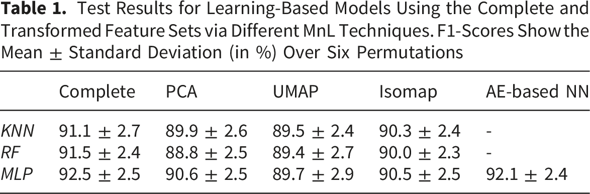
Test Results for Learning-Based Models Using the Complete and Transformed Feature Sets via Different MnL Techniques. F1-Scores Show the Mean ± Standard Deviation (in %) Over Six Permutations
To thoroughly assess the performance of the MLP model, Figure 3 presents a full range of evaluation metrics for two feature set configuration: the complete and the AE-based NN transformed, including training set results. By comparing metrics across training and test sets, we can examine potential overfitting: larger discrepancies between these sets typically indicate reduced generalization capability, as the model may struggle to perform consistently on unseen data. The figure suggests minimal overfitting in the MLP model, as performance metrics remain stable across both sets. This stability is largely attributed to the test permutation procedure, which helps mitigate the potential for overfitting. The AE-based NN stands out by maintaining overall scores comparable to those achieved with the complete feature set, and even exhibiting a slight increase in precision. This suggests that this approach effectively retains essential discriminative features, thereby facilitating robust detection of TN. Comparison of train and test results for MLP performance across the complete dataset and AE-based NN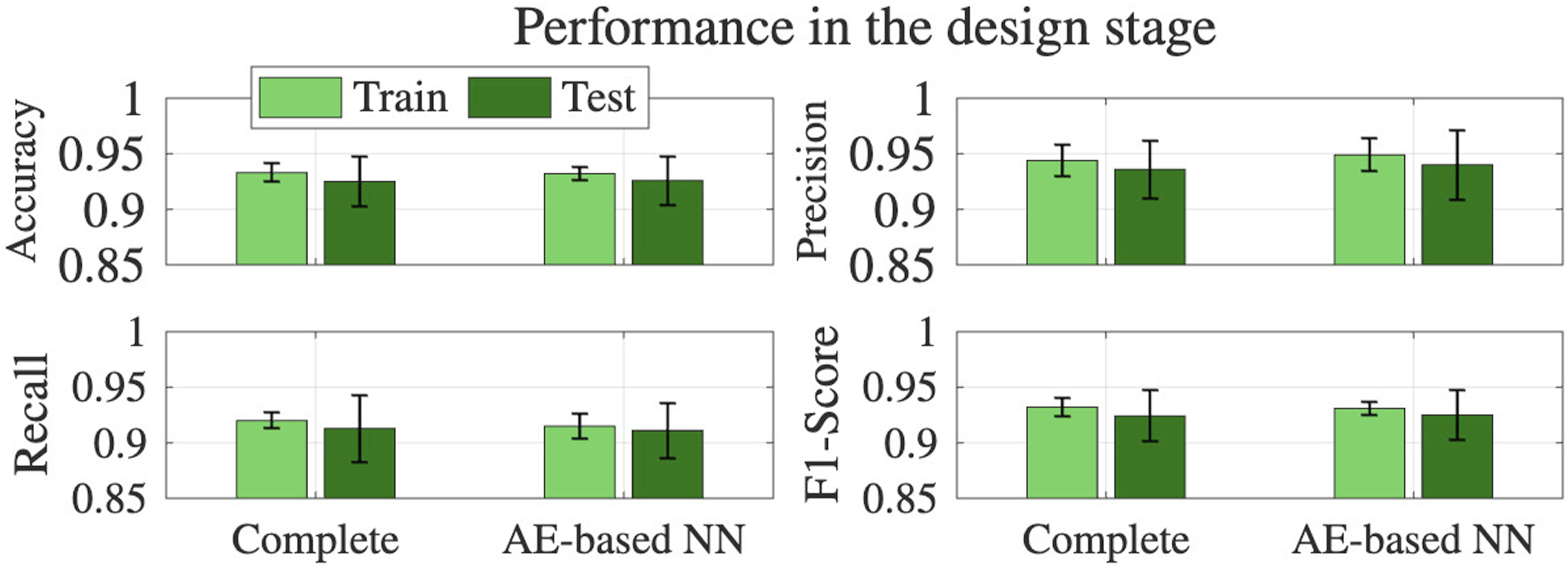
To complement these observations and statistically validate the performance differences between the complete and reduced feature sets, we conducted paired t-tests and Wilcoxon signed-rank tests across six patient-based permutations. The statistical analysis further confirms that the AE-based NN decrease in F1-score is not significant (t-test: p = 0.7187; Wilcoxon: p = 0.8438), reinforcing its strength in retaining essential discriminative information. In contrast, UMAP, PCA, and Isomap show statistically significant drops in performance (all p < 0.01 in t-tests; p = 0.0312 in Wilcoxon tests), reflecting a consistent degradation in classification capability when using only three components. The Wilcoxon test, being non-parametric and robust to outliers, supports the same conclusion as the t-test, lending robustness to the findings. These results position the AE as the most effective among the explored MnL techniques, offering dimensionality reduction and interpretability with minimal compromise to predictive accuracy.
The use of MnL introduces a new level of explainability to the machine decision process, which was previously obscured by the full set of 14 features. By reducing this space to three dimensions, we can now project the instances and obtain some insight of the classifier decisions. In Figure 4, the predictions made by the MLP on both the train and test sets after manifold application are projected onto this latent space. The displayed decision boundary, established after training, demarcates regions where the classifier considers predictions to be either positive or negative. Moreover, the visualization reveals a clear relationship between prediction accuracy and distance from the decision boundary: true predictions (TPs and TNs) lie farther from the boundary, while misclassifications (FPs and FNs) cluster closer to it, indicating higher uncertainty. This consistent clustering pattern across all MnL approaches for the different categories highlights a strong correlation between classifier confidence and the distance from the decision boundary. Projection of MLP classifier predictions during the design stage using two MnL techniques: UMAP (top) and Isomap (bottom). Each subplot displays predictions for both training set (left) and test set (right). Samples are colored according to confusion matrix categories and the MLP decision boundary is shown in the embedded space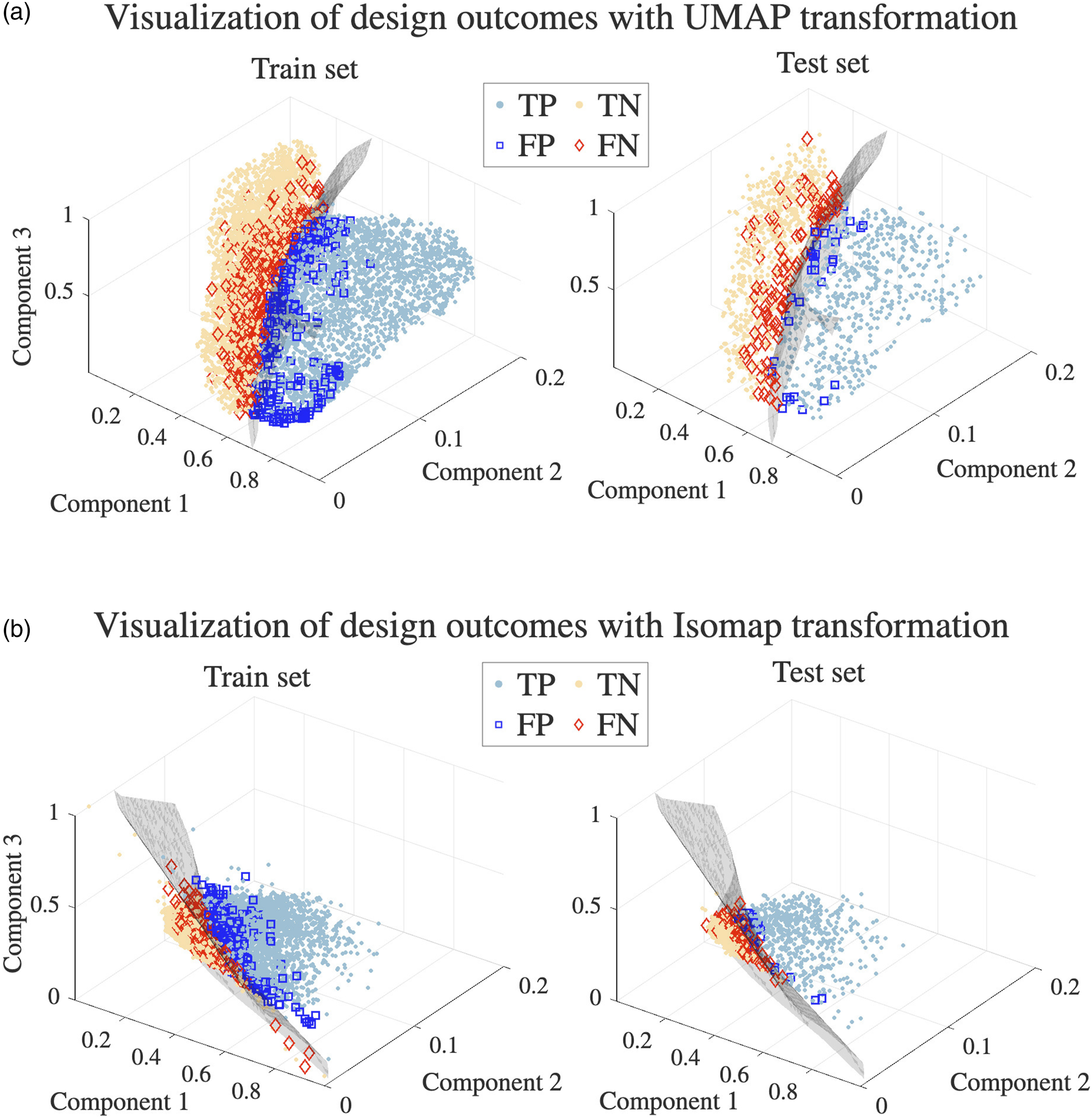
The MnL-generated spaces visualization demonstrates clear differentiation between voltage levels in machine predictions as well. Figure 5A focuses exclusively on false predictions, applying UMAP to visualize FNs at extreme voltage levels of 20 μV and 80 μV to heighten contrast. It is important to note that FPs are not associated with a specific voltage value, as they indicate the absence of TWA, corresponding to a voltage of 0 μV. As anticipated, a higher number of undetected episodes occur at lower amplitudes, with only a few missed episodes at 80 μV and even fewer at higher amplitudes. Additionally, mispredictions for lower amplitudes are more widely dispersed in the space, especially for the test set, indicating a greater classification difficulty. In contrast, higher-amplitude misses tend to cluster nearer to the decision boundary, suggesting they were closer to correct classification, which further highlights the relative ease of detecting higher-amplitude alternans. Combined visualization of false predictions: (A) false predictions visualization by the MLP using UMAP. FP and FN at 20 μV and 80 μV TWA episodes are shown for train (left) and test (right) sets; (B) FN histogram stratified by TWA voltage, comparing MLP with AE-based NN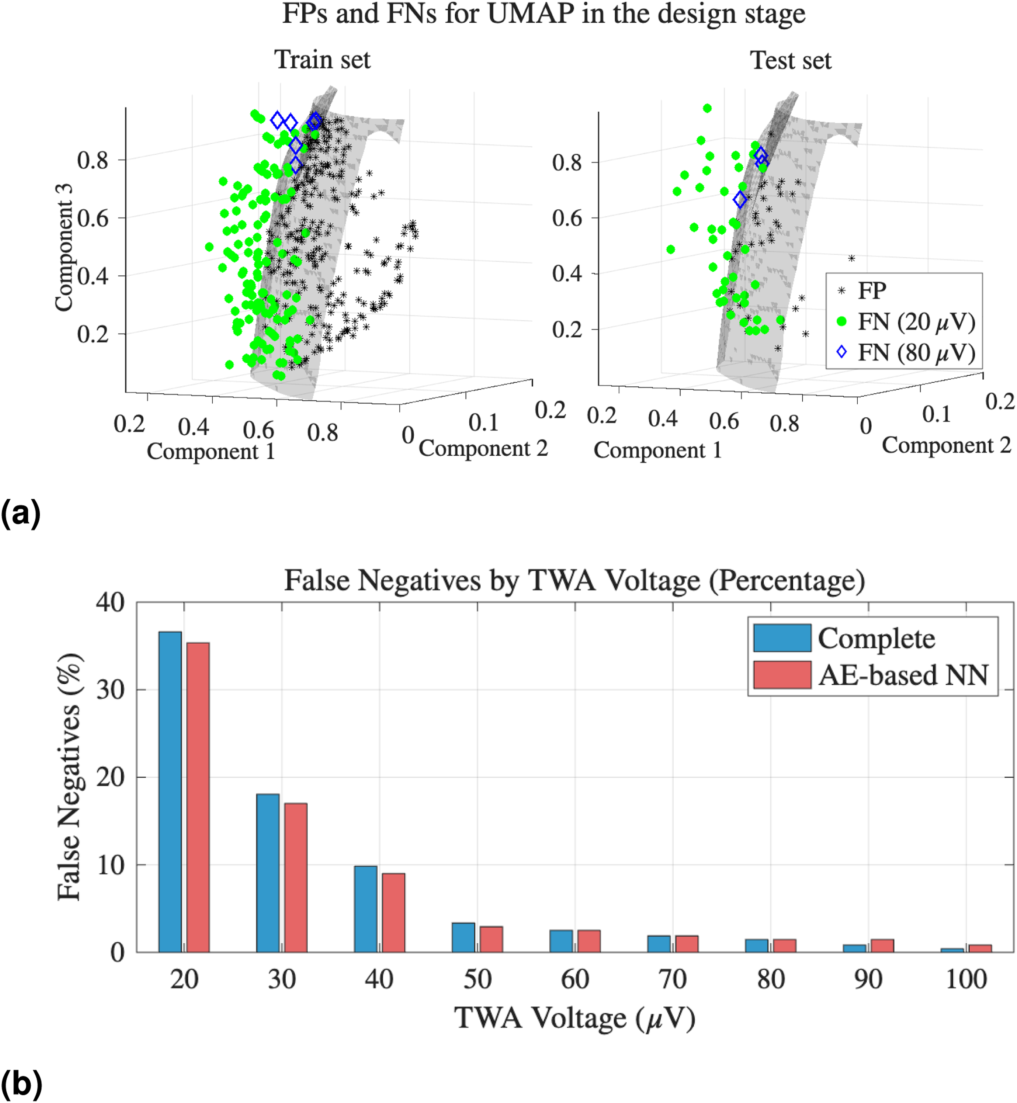
This observation, that most missed events are linked to lower-voltage alternans, aligns with the voltage-wise FN analysis presented in Figure 5B. This figure quantitatively compares the distribution of missed TWA detections between the original model (complete set) and the most competitive one, the AE-based NN. Interestingly, while both models exhibit most errors at low TWA amplitudes, the AE-based model demonstrates slightly fewer FN in this low-voltage range, suggesting improved sensitivity to subtle alternans. However, the original MLP generally outperforms the AE-based model at higher voltages, where it achieves near-complete detection. This trade-off illustrates how the AE-based approach may improve detection in more ambiguous, low-amplitude scenarios, while the complete MLP retains an advantage in clearer, high-amplitude cases. Nonetheless, statistical analysis indicates that their overall performance remains closely comparable.
4.2. TWA Detection on Real Ambulatory Environment
The performance of the trained models for detecting TWA episodes in ambulatory recordings is detailed in this section. As mentioned in Section 3.2, TWA events are now integrated into the signal in a sparse and non-sustained manner, reflecting realistic clinical conditions. This presents a significant challenge for detection compared to sustained events. We also employed the patient permutation procedure to enhance the robustness of our results, allowing us to report mean and standard deviation outcomes. The test results shown reveal the effectiveness of our models in accurately identifying TWA episodes while effectively filtering out FPs through the described post-processing steps.
Performance of TWA Detection in Ambulatory Environments on the Test Set, Evaluated in Terms of Precision, Recall, and F1-Score (in %) for Various Feature Sets Using the Best ML Model for Each Set
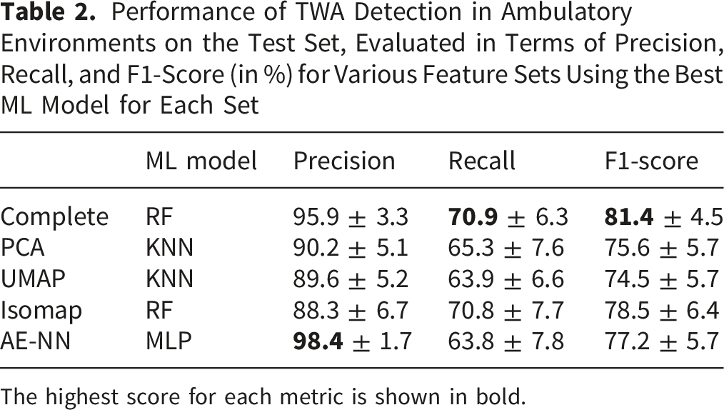
The highest score for each metric is shown in bold.
Our analysis now shifts to the interpretability offered by the AE-based NN, with a focus on its decision-making process. This method demonstrates not only a consistently strong F1-score but also the highest precision among all MnL approaches, highlighting its capability in minimizing FPs and enhancing the reliability of the detection mechanism. Figure 2 illustrates an example of TWA detection applied to an ambulatory signal, showing the beat series tracking where the TWA pattern is visible. While the model successfully detects some of the TWA episodes, there are a few false predictions and undetected episodes, the latter being attributed to the consistency constraints imposed on the predictions. Figure 6 visualizes the latent space generated by our model, showing the positions of the instances within this learned space. The decision boundary, established during the model design phase, determines whether an instance is classified as negative (red cross) or positive (blue circle), effectively separating the instances. A critical aspect of this analysis is the post-processing step, where the predictions are refined into detections. As observed, only the green-filled points represent true detections, as they have successfully passed the post-processing test. Interestingly, these detections tend to lie on the far side of the decision boundary, indicating a higher confidence in the model predictions. In contrast, instances closer to the boundary are less likely to be classified as detections, demonstrating the model ability to assess prediction certainty. This thorough examination of the model decision-making process not only bolsters our confidence in its explainability but also validates our FP filtering method, which effectively minimizes incorrect detections. Explainability analysis for the AE-based NN TWA detection outcome in Figure 2. Latent space projection is shown, providing insights into the model decision-making process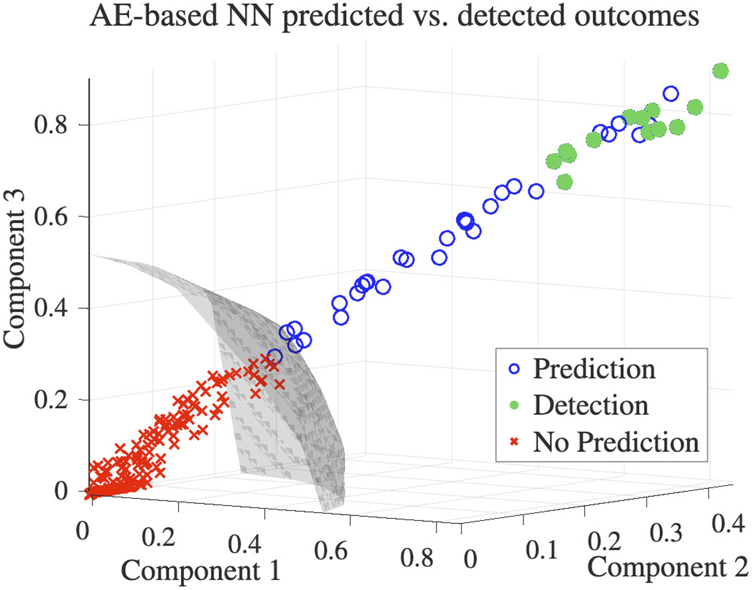
5. Discussion
MnL is a robust approach for mapping high-dimensional data into low-dimensional embedded spaces, making complex datasets more interpretable and accessible. In contexts like ours, where high-dimensional data can obscure underlying structure and meaning, MnL techniques play a crucial role by distilling essential features and uncovering patterns that would otherwise remain hidden. This explainability is particularly valuable in healthcare applications, where transparent and comprehensible models foster trust, enhance clinical decision-making, and ultimately support better patient outcomes. In this work, we have developed an initial yet powerful framework by generating and analyzing the embedded spaces of ECG data, exploring how instances are distributed within these spaces based on the presence of TWA episodes. To accomplish this, we have compared a range of MnL techniques, each with its own methodology, resulting in distinct and unique data representations, but consistently preserving underlying patterns. A key strength of our approach is the careful attention given to optimizing these techniques through an in-depth investigation of how different parameter configurations impact the results. This effort ensures that the full potential of MnL is harnessed. By uncovering patterns that correlate with TWA events, our approach has the potential to enhance early detection and monitoring of risk factors, ultimately improving clinical decision-making and patient outcomes. While we do not directly provide interpretability with the findings in this study, our framework enables further exploration into the ECG embedded space, setting the stage for future studies aimed at refining TWA detection. By advancing both the explainability and clinical relevance of TWA analysis, this groundwork supports the development of more effective, reliable detection methods that are critical for managing patient cardiac health.
The visualization of ECG instances in the embedded space has provided valuable insights into their distribution, an analysis that had not been conducted previously. This approach allows us not only to observe how the model differentiates between TWA and non-TWA instances, but also to uncover hidden patterns in the amplitudes of TWA events. One such pattern, while seemingly intuitive, had not been explicitly confirmed before: the model struggles most with micro-alternans. We have confirmed that the model tends to position mispredictions near the decision boundary, indicating a degree of uncertainty. Interestingly, within these false predictions, low-amplitude TWA events are placed farther from the boundary than high-amplitude events. This suggests that while the model exhibits indecision, the errors tied to smaller-amplitude TWA events are more pronounced compared to those involving higher-amplitude mispredictions. These findings emphasize the challenge machines face in detecting micro-alternans, suggesting that our results would be significantly stronger if not for the challenge posed by smaller-amplitude TWA events, which uniquely impact detection performance. By recognizing these challenging cases, such as low-amplitude TWA events, more attention can be focused on them in future iterations of the model. Additionally, factors such as clinical history, gender, and age could be explored to gain deeper insights into their influence on model performance. Given that patients with similar ages or the same gender may naturally cluster together, analyzing these variables could reveal underlying patterns that impact classification. This targeted focus could lead to improvements in handling these difficult instances, ultimately strengthening the overall performance of the model and addressing its current weaknesses.
We also emphasize the disparity in performance metrics between two scenarios. In Section 4.1, classifiers learn from a balanced dataset. In contrast, in Section 4.2, the events are sparse, reflecting conditions typically encountered in clinical practice, and the results are obtained using pre-trained classifiers. These experiments are essential to effectively translate the methodologies into clinical applications, yet they are often overlooked in research.
Our contribution paves the way for further advancements in TWA detection, with a particular focus on better understanding the results. Although TWA detection is a critical area, it remains significantly underexplored, primarily due to the absence of real annotated data needed to validate and enhance algorithm performance. Therefore, it becomes clear how crucial it is to establish a gold-standard method for TWA detection. Such a benchmark would provide a reliable reference for validating and comparing detection algorithms, while also supporting the development of more accurate models. Given that our current models perform satisfactorily and offer reliable detection through multiple trained systems, applying them to real-world signals from patients at risk of SCD would represent a significant step forward. This would not only validate our approach in a clinical setting but also help assess its potential to improve patient outcomes in high-risk scenarios.
Nevertheless, the primary limitation of our study is the lack of real-world ECG data with annotated TWA events, which constrains our ability to thoroughly evaluate and enhance the proposed methods. Although we design TWA episodes to closely resemble real-world conditions, certain aspects of the signal model remain simplified, such as the assumption of constant alternans amplitude within each episode, which could be further refined to better capture physiological variability. Moreover, the scope of our dataset is still constrained compared to what could be achieved with larger and more diverse real-world datasets, which also contributes to the observed performance gap between the controlled design stage and the more challenging ambulatory scenario. As a future direction, we aim to establish collaborations with clinical institutions to collect long-term ECG recordings from patients identified as having elevated cardiac risk profiles, using wearable devices in real-life settings. Applying our methodology to these real-world signals would allow for the detailed characterization of alternans under naturalistic conditions. In this context, a more direct linkage between latent-space structures and electrophysiological markers of repolarization would constitute a valuable extension of the present work. It would also allow us to further assess the generalizability of the learned representations and strengthen the clinical validity of our detection framework. Furthermore, by correlating alternans patterns with patients’ clinical histories, we may uncover clinically meaningful trends that contribute to improved risk stratification and early detection strategies.
Given the current data limitations, we have concentrated on simpler, lightweight ML models that are more suited to smaller datasets. While these models have yielded valuable insights, more sophisticated deep learning models could potentially offer even greater accuracy by capturing more intricate patterns in the data. However, employing such advanced models depends on access to a sufficiently large and diverse dataset, which is essential to train them effectively, avoid overfitting, and fully harness their potential. Despite this limitation, our findings underscore the strong foundation laid by our current approach and the clear potential for further advancements in TWA detection. Notably, the dataset expansion we implemented from previous work resulted in significant performance improvements, indicating that our methods are highly responsive to increases in data availability. This highlights the promise of further gains with larger annotated datasets. Importantly, our use of explainable, simpler models has already provided meaningful insights into the detection process and set a scalable baseline. Looking ahead, the groundwork established here positions our framework to benefit from future data availability and to evolve alongside more complex modeling techniques, ultimately moving us closer to practical solutions for managing patient cardiac health.
6. Conclusion
The experiment conducted in this project effectively demonstrates the successful application of learning-based methods to detect TWA episodes in real-world settings through in-line analysis. By extending our previous approach of overlapping instances into the design stage, we have unified the methodology across both the design and deployment phases of the models, resulting in a substantial increase in the training dataset size. This increase has translated into significant improvements in detection performance and offers optimism for even better performance with more data. A key contribution of this work is the introduction of embedded spaces using MnL techniques, which significantly enhance the explainability of the models. This innovation provides greater transparency into the decision-making process without substantially compromising detection accuracy. Not only does this improve the reliability of our models, but it also helps identify their potential weaknesses, thus enabling targeted refinements to further enhanced performance. Our work establishes a robust methodological framework through meticulous fine-tuning of both MnL and ML parameters, providing a solid foundation for developing a clinically validated ground truth method for TWA detection.
Looking ahead, future efforts could focus on applying this methodology to long-term ECGs from high-risk patients using wearable devices, aiming to validate model generalizability and explore clinical correlations with patient outcomes for better risk stratification. Expanding the dataset would also enable more advanced deep learning models to capture complex features and improve accuracy. The observed gains with increased data highlight the potential of ongoing data collection and refinement to make this approach a clinically valuable tool for cardiac monitoring.
Footnotes

Author Contributions
RGE, LPS, and MBV conceived, designed, and performed the experiments. All coauthors analyzed and interpreted the data, contributed reagents, materials, analysis tools or data, and also all coauthors wrote the paper.
Funding
The authors disclosed receipt of the following financial support for the research, authorship, and/or publication of this article: This work has been partially supported under research project grant PID2022-140786NB-C32 by MCIN/AEI/10.13039/501100011033.
Declaration of conflicting interests
The authors declared no potential conflicts of interest with respect to the research, authorship, and/or publication of this article.
Data Availability Statement
Data available on request from the authors.